mixings and decays in private Higgs model
Abstract
We study the low energy phenomena induced by the lightest charged Higgs in the private Higgs (PH) model, in which each quark flavor is associated with a Higgs doublet. We show that the couplings of the charged Higgs scalars to fermions are fixed and the unknown parameters are only the masses and mixing elements of the charged Higgs scalars. As the charged Higgs masses satisfy with , processes involving -meson are expected to be the ideal places to test the PH model. In particular, we explore the constraints on the model from experimental data in physics, such as the branching ratio (BR) and CP asymmetry (CPA) of , mixings and the BR for . We illustrate that the sign of the Wilson coefficient for can be different from that in the standard model, while this flipped sign can be displayed by the forward-backward asymmetry of with a vector meson. We also demonstrate that mixings and their time-dependent CPAs are negligible small and the BR of can have a more strict bound than that of .
I Introduction
The masses of quarks and charged leptons are dictated by the Yukawa sector in the standard model (SM) through the simple and elegant Higgs mechanism, where the vacuum expectation value (VEV) of the Higgs field, determined by massive gauge bosons, indicates the scale of the electroweak symmetry breaking (EWSB) with GeV. According to the data, there appear mass hierarchies in the generations of charged fermions such as , and , while and but PDG08 . In the SM, due to the scale of the EWSB being fixed by the VEV of the Higgs field, the mass hierarchies are ascribed to the finetuning of the Yukawa couplings.
In the Cabibbo-Kobayashi-Maskawa (CKM) matrix CKM , defined by with the unitary matrix for diagonalizing the quark mass matrices, it is known that the off-diagonal elements denoted by are suppressed by the Wolfenstein parameter Wolfenstein . If the effects of are turned off, one immediately finds . In other words, small elements of imply that the structures of the Yuwaka matrices for up and down type quarks should be close to each other. However, based on the above discussion, the similarity of the mass structures is not respected by the data. Plausibly, we need to extend the Yukawa sector to explain the mass hierarchies.
In order to evade the drawback of the finetuned Yukawa couplings, a new type of solutions to the mass hierarchy is recently proposed in Refs. PZ1 ; PZ2 , in which the authors extend one Higgs doublet in the SM to multi-Higgs doublets with each gauge singlet right-handed fermion associated with one Higgs doublet. Hereafter, the model is called as the private Higgs (PH) model PZ1 . The philosophy of solving the mass hierarchies in generations is now to utilize the hierarchy of VEVs of scalar fields instead of the hierarchy of the Yukawa couplings. Although many new neutral and charged scalar bosons are introduced in the PH model, most of the effects are suppressed by the heavy masses. In addition, the PH model provides the candidate of dark matter. The detailed study could be referred to Ref. Jackson .
Since top and bottom quarks are the first two heaviest fermions, the dominant new effects are expected to be associated with the Higgs doublets, denoted by , respectively. Since implies , gives the dominant new physical effects if we take as the SM Higgs. Accordingly, we anticipate that the B-meson system could be the good environment to probe the special character in the PH model. In this paper, we study the effects of the private charged Higgs bosons on the rare flavor changing neutral current (FCNC) processes, such as mixings and decays with q=s, d. These processes are expected to be sensitive to the charged Higgs sector.
II Charged Higgses in private Higgs model
To examine the charged-Higgs effects in the PH model, we first review the model proposed in Ref. PZ1 . In the model, as the hierarchy of the scalar VEVs is used to understand the fermion masses instead of the arbitrary Yukawa couplings, the SM with one Higgs doublet is extended to include six Higgs doublets so that each Higgs doublet can only couple to one flavor with imposing a set of six discrete symmetries. In addition, six gauge singlet real scalars are introduced to achieve the spontaneous symmetry breakings. For simplicity, we will take only one singlet scalar field in our discussion. The six-singlet case can be easily accommodated but our results on FCNCs remain the same. Under the discrete symmetries, the transformations for the flavor and the scalars are set to be
| (1) |
where denotes the possible flavor of the quark, is the associated Higgs doublet scalar and S is the gauge singlet scalar. Since the left-handed quark belongs to the doublet of two flavors, we require that it is invariant under the discrete transformations. Accordingly, the related scalar interactions with the electroweak gauge and discrete symmetries are given by PZ1
| (2) | |||||
where is the covariant derivative, is the mass of , is the VEV of S, is a free parameter, the values of , , and are regarded as the same order of magnitude, and stands for the Yukawa sector to be given. Since the top quark is the heaviest quark with its mass close to the EWSB scale, it is natural to take as the Higgs doublet in the SM. Therefore, to develop a nonzero VEV of to have the EWSB spontaneously, the condition of should be satisfied. Consequently, the relevant scalar potential with the leading terms is given by
| (3) |
By minimizing Eq. (3), the VEVs of S and are obtained as
| (4) |
We now discuss how to get the small VEVs for . Unlike the case for , we need to adopt the condition for . The relevant subleading scalar potential for is
| (5) |
We note that although the coefficients of , and are similar to in magnitude, their effects are sub-subleading and negligible due to the associated VEVs of scalar fields being much less than . Similarly, by minimizing Eq. (5) the VEV of is given by PZ1
| (6) |
Clearly, if we set to be the same order of magnitude for a different , the hierarchy of VEVs could be obtained by controlling , i.e., the heavier is, the smaller will be for .
After introducing the strategy to obtain the EWSB spontaneously as well as the small VEVs of the scalar fields with , we can proceed to investigate the characters of the charged Higgs scalars in the PH model. In terms of gauge symmetries, the Yukawa sector is given by
| (7) |
where and denote the doublet and singlet of , respectively, and is the Yukawa matrix for down (up) type quarks. In the flavor space, are also matrices, given by
| (14) |
where and are the Higgs doublets of , which couple to and , respectively. After the EWSB with the shifted scalar fields
the mass terms of quarks in the Yukawa sector are developed to be
| (15) |
with
| (19) |
To avoid the large FCNCs at tree level, we adopt the Yukawa matrices in Ref. PZ1 , given by
| (20) |
where and , and . By combining with , the quark mass matrices can be simplified as
| (27) |
where correspond to the light quarks and the first two heaviest quarks, and . To get the physical states, we use and to diagonalize the mass matrices, i.e. and . The individual informations on and can be obtained by
| (28) |
respectively, where
| (35) |
with . Due to , it is a good approximation to take . Furthermore, from Eq. (35), one observes that the off-diagonal elements of are much larger than those of and thus, and . As a result, at the leading order approximation the right-handed unitary matrices could be taken as identity matrices. Consequently, we obtain
| (36) |
It is clear that the induced FCNCs at tree level due to the Yukawa terms are suppressed by . Although we cannot get a simple relation for with , the FCNCs, involving the first two generations at tree level, will be suppressed by the heavy masses of . The detailed analysis on the neutral Higgs exchange can be found in Ref. PZ1 .
In order to demonstrate that the neutral Higgs mediated FCNC effects will not impose a further serious constraint on the parameters for the charged Higgs, below we give an explicit discussion on the mixing. According to Eq. (7), the relevant Yukawa terms are given by
| (37) |
where denotes the flavor of d-, s- and b-quark. Due to being the next lightest scalar, in terms of mass eigenstates the dominant effects for FCNCs at tree level in the processes are written by
| (38) |
From the previous analysis, since the off-diagonal elements of the flavor mixing matrix for the right-handed quark are small, Eq. (38) only involves the flavor matrix matrix of . Using Eq. (20) and , we see that
| (39) |
Furthermore, with the result of shown in Eq. (36), we find that the -mediated FCNCs not only are associated with the parameter , but also appear in . As a result, the contributions to the mixing are proportional to . Clearly, by choosing some suitable small value of and , they could be smaller than the current data. In other words, the neutral Higgs mediated processes will not provide a further constraint on the parameters for the charged Higgs related effects.
Now, we only pay attention to the charged Higgs related effects. With the physical eigenstates of quarks, the charged Higgs interactions to quarks can be found in Eq. (7), given by
| (40) |
where is a matrix and its definition is similar to Eq. (14). We note that does not represent the physical charged Higgs scalars. Since there are six Higgs doublets in the model, basically we have 5 physical charged Higgs scalars and one charged Goldstone boson, which is usually chosen to be
| (41) |
with . Therefore, to study the effects of physical charged Higgses, in general, one needs to consider a mass matrix for these charged scalar fields. According to our earlier analysis, the hierarchy of quark masses is represented by the hierarchy of VEVs of the scalar fields. Due to , it should be a good approximation to take , i.e., almost aligns to the Goldstone boson. Then, the lightest charged Higgs will be the . Moreover, since , the scalar mixing effects associated with could be neglected due to the suppression of their heavy masses. Based on the character of the PH model, the interesting effects of the charged Higgses are in fact only associated with , and . Effectively, the charged Higgs mass matrix is a matrix, which is similar to that in the Weinberg three-Higgs-doublet model Weinberg . Interestingly, if we further neglect the effect of , the situation returns to the conventional two-Higgs-doublet model Lee . By using Eqs. (20) and (36), we obtain that diag(. Moreover, from Eq. (40), we find that the sizable effects due to the charged Higgs scalars are related to and , where the vertex for the former is given by while the latter . It has no doubt that the coupling is dominated by k=3. However, it is more complicated for the coupling . To see it, we take with the sum
| (42) | |||||
In terms of Eq. (36), the CKM matrix can be expressed by . Accordingly, we get . Thus, in the phenomenological analysis, we can choose a suitable value of so that . The dominant effect for the vertex of could be simplified to be , i.e., the 3-3 element of is the main contribution.
In order to compare with the conventional two-Higgs-doublet model, we rewrite Eq. (40) in terms of quark masses and Eq. (19) as
| (43) |
If we take and , we can easily get the formulas for the charged-Higgs interactions in the two-Higgs-doublet model to be
| (44) |
Furthermore, by using the relationships of
| (45) |
with , and , we have
| (46) | |||||
III Phenomenologies in B decays
According to the discussions in Sec. II, we know that there is an essential difference in the couplings of the charged Higgs scalars and quarks between the conventional multi-Higgs and PH models. For instance, if we turn off the CKM matrix elements, from Eq. (40) we see clearly that the couplings in the former are directly proportional to the masses of quarks but those in the latter do not involve new free parameters in the leading contributions. In addition, in the former case, there are no intrinsic limits on the charged Higgs masses, whereas in the latter case, the masses have a preceding hierarchy stemmed from Eq. (6). Consequently, we speculate that the lightest charged Higgs scalar with the couplings of order one in the PH model might have interesting phenomenologies in rare decays suppressed in the SM. From Eq. (40), one can easily find that the large novel effects are associated with t and b quarks and the corresponding charged Higgs scalars are mostly the first two lightest ones of and . Hence, in the following analysis, we will concentrate on the rare -meson processes involving FCNCs due to the charged Higgs scalars.
III.1 mixings
It is known that all neutral pseudoscalar-antipseudoscalar oscillations in the down type quark systems have been seen. In the SM, since the oscillations are induced from box diagrams, they are ideal places to probe the new physics effects. As mentioned early, since are much heavier than , their contributions to the processes in the -system are small, whereas significant contributions in the B-system could be possible.
To calculate (q=d, s) mixings in the PH model, we first consider the diagrams displayed in Fig. 1 due to the gauge and charged Higgs bosons in the loop. The crossed diagrams of internal bosons and fermions are included in the calculations but not explicitly shown up in the figures. To see the mixing effects of the charged Higgs scalars, we present the diagrams in terms of unphysical states. However, we will formulate the results based on the physical ones. Since Figs. 1(b) and (d) involve the heavy charged Higgs , the contributions must be much smaller than those by Figs. 1(a) and (c) and therefore, they can be ignored.
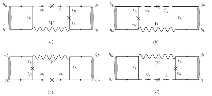
The effective four-fermion interactions for from Figs. 1(a) and (c) are given by
| (47) | |||||
with
where , and denotes the unknown mixing element between and . As discussed early, if we regard that the effective charged Higgs scalars are , and , their mixtures are similar to those in the Weinberg’s three-Higgs-doublet model. In general, is a complex number. Here, for simplicity, we have only shown the contributions of the lightest physical charged Higgs denoted by , referred as private charge Higgs. Besides Fig. 1, the diagram in Fig. 2 also yields an important contribution to the mixing. From Eq. (40), we find

| (48) |
with
To examine the oscillating effect, we parametrize the matrix elements as Masiero
| (49) |
where , and is the decay constant of . Accordingly, the matrix elements of and are given by
| (50) |
where
| (51) |
with the gauge coupling of . We note that because has the suppression factor of , it is much smaller than . In the following analysis, we will neglect the contribution of .
To study the influence of new physics on the time-dependent CPA, we write the transition by combining results from the SM and new physics as
| (52) |
where is the weak CP phase of the SM, corresponds to the new CP phase in the PH model and is given by
| (53) |
with and . Due to in the B-system PDG08 , the time-dependent CPA is found to be
| (54) |
with and . From Eqs. (50) and (51), one gets that and
| (55) |
which is independent of in the PH model. From Eq. (54), it is readily seen that the magnitude of is controlled by .
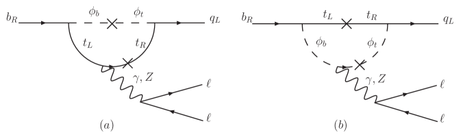
III.2 decays
It is known that decays provide strong constraints on the penguin contributions from new physics. In this subsection, we examine these decays in the PH model. As an illustration, we present the possible dominant effects in Fig. 3. From the figure, we see clearly that Figs. 3(a) [(c)] and (b) [(d)] involve chirality flip of [] and the mixing of and []. Due to and the mixing effect of and () being much smaller than that of and (), the contributions of Figs. 3(a) and (b) are much smaller than those of Figs. 3(c) and (d). Therefore, to study the leading effects, the results of Figs. 3(a) and (b) can be neglected. Furthermore, if we replace photons in Fig. 3 with gluons, gluonic penguins can be also generated by the charged Higgs scalars in the PH model.
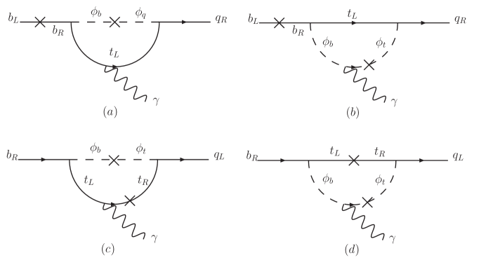
From Figs. 3(c) and (d), we conclude that the effective operators from the charged scalars have the same structures as those in the SM. In order to include the SM contributions, we write the effective Hamiltonian for as BBL
| (56) |
where are the effective operators at scale and are the corresponding Wilson coefficients. Because the dominant effects of the SM are from the terms with , and , we only show the associated operators of
| (57) | |||||
| (58) |
respectively, where , is the electric charge, is the strong coupling constant, and denote the color indices, with a=1,…,8 are the generators of the gauge symmetry and () is the electromagnetic (gluonic) field strength. The effective Wilson coefficients by combining the contributions of the W-boson and lightest charged Higgs are given by
| (59) |
with
| (60) |
where denotes the SM result, is the electric charge of the top quark and the loop integrals and come from Figs. 3(c) and (d), given by
| (61) |
respectively.
III.3 and decays
In this subsection, we discuss the leptonic and semileptonic decays. The effective Hamiltonian for in the SM is given by BBL ; CG_NPB636 ; CG_PRD66
| (62) |
with
| (63) |
where , is the invariant mass of the lepton-pair and , and are the Wilson coefficients (WCs) with their expressions for next leading order corrections in Ref. BBL . Since the operator associated with is not renormalized under QCD, it is the only one with the scale free. In addition, by considering the effects from the one-loop matrix elements of and , the resultant effective WC of is BBL
| (66) | |||||
with and . Similar to the SM, electroweak penguin diagrams in Fig. 4 mediated by the private charged Higgs scalars can also contribute to . Therefore, in terms of Eq. (40) and the mixture of and , the results of Z- and -penguin are formulated to be
| (67) |
respectively, with
| (68) |
and
| (69) |
where is the third component of weak isospin and is the electric charge of .
With the effective interactions in Eqs. (62) and (67) for , the BR for the two-body decay is straightforwardly given by
| (70) |
with
Since the BR is proportional to the lepton mass, obviously, the related decays are chiral suppressed. In addition, we see that only the mediated Z-penguin has the contribution to the decays. In order to study , we have to know the information on the transition elements of with various transition currents. As usual, we parametrize the relevant form factors as follows:
| (71) |
where , are the masses of , pseudoscalar and vector mesons, , respectively, and . By equation of motion, we can have the transition form factors for scalar and pseudoscalar currents as
| (72) |
Here, the light quark mass has been neglected. According to the definitions of the form factors, the transition amplitudes for can be written as
| (73) |
with
| (74) |
and
| (75) |
where
| (76) |
with
| (77) |
Here, we only pay attention to the light leptons with the explicit effects of ignored.
To get the decay rate distribution in terms of the dilepton invariant mass and the lepton polar angle , we use the rest frame in which , with , and . By squaring the transition amplitude in Eq. (73) and including the three-body phase space factor, the differential decay rate as a function of and for is given by
| (78) |
For , by summing up the polarizations of with the identity , from Eq. (75) the differential decay rate is found to be
| (79) | |||||
Here, ( or ) represents the spatial momentum of the meson in the -meson rest frame, given by with . The forward-backward asymmetry (FBA) is defined by
| (80) |
with . Since Eq. (78) has no linear term in , the FBA for vanishes. Hence, only has a nonvanished FBA, given by
| (81) | |||||
IV Numerical results and discussions
Since the contributions to the processes in the mixing, , and by the charged Higgs scalars have strong correlations, the new free parameters are only and . On the other hand, we can find constraints among these decays due to experimental data. To comprehend the influence of the new charged Higgs on the rare decays, we in turn investigate the above processes. As an illustration, we only focus on the processes with .
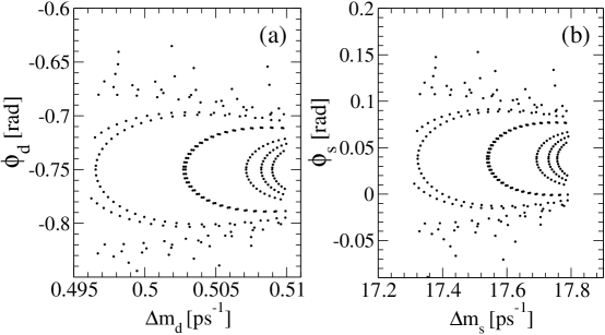
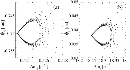
For the mixing, besides the mass difference of two physical B-meson states described by , the time-dependent CPA in Eq. (54) is also an important physical quantity to display the new physics. To do the numerical analysis, we take GeV, GeV, with and with HFAG , in which the leading SM results are ps-1 and ps-1. Accordingly, we present the influence of the private charged Higgs in Fig. 5, where , is set to be 150 GeV 1 TeV and and have been chosen to satisfy ps-1 and ps-1 CDF ; D0 . We note that although has a very high precise measurement with ps-1 PDG08 , since the error from the nonperturbative QCD is large, for theoretical estimations we take a conservative bound. From the figure, we see clearly that if we only consider the constraints of , the CP phases extracted from time-dependent CPAs of have significant deviations from those in the SM.
It is known that the BR for not only has been measured well to be HFAG but also is consistent with the SM prediction of bsgaSM . Hence, could give a strict constraint on the parameters of new physics. To simply get the bound, we adopt the BR for to be KN
| (84) |
where denotes the fraction of the spectrum above the cut, , is a phase-space factor, stands for the next-leading-order (NLO) effect, is the NLO effect of and the values of and are given in Table 1. Here, we have only considered the case with .
| 0.30 |
|---|
According to the results in Ref. KN , the relevant Wilson coefficients with charged Higgs contributions are found to be
| (85) |
We can also investigate the direct CPA for , given by KN
| (86) | |||||
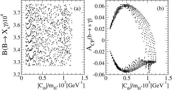
where the current data is HFAG . Since the SM prediction is less than Soares , the formula in Eq. (86) has neglected the contributions related to the KM phase. If any sizable CPA is found, it definitely indicates the existence of some new CP violating phases. For , we first display versus in Fig. 6. From the figure, it is clear that the BR of has a very serious constraint on and so that the contributions of the private charged Higgs to the time-dependent CPA become very small.
To further understand the effects of the charged Higgs on the radiative B decays, we show the correlation between [] and in Figs. 7(a)[(b)]. Interestingly, those values of parameters, which are satisfied with the bound of , could still make at few percent level where the sensitivity is the same as the current data.
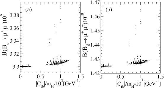
Next, we study the implications of the private charged Higgs on . According to the previous analysis, we learn that and could give strong bounds on the free parameters in the PH model. With the constraints, we show the BRs for in Figs. 8(a) and (b). From the figures, we see that the contributions in the PH model are very close to in the SM. Hence, we conclude that the effects of Z-penguin in Fig. 4 are negligible.
To estimate the numerical values for decays, we use the form factors calculated by the light cone sum rules (LCSRs), parametrized by LCSR
| (87) |
with the associated values of parameters given in Table 2 and 3 for and , respectively.
| GeV2 | GeV2 | ||||
|---|---|---|---|---|---|
| GeV2 | GeV2 | ||||
|---|---|---|---|---|---|
From Eqs. (78) and (79) and with the same values of parameters for , we present the influence of the private charged Higgs on in Fig. 9. We find that the charged Higgs in the PH model has significant effects on the BRs for . Since the contributions from mediated Z-penguin are very small, the main enhancements come from the -penguin appearing in of Eq. (60) and of Eq. (68).
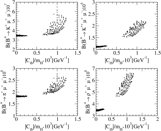
By comparing with the current experimental data, expressed by PDG08 ; HFAG
| (88) |
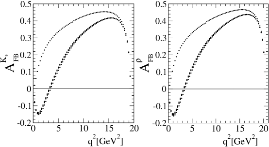
we find that the BR of in the PH model could be larger than the upper value of the current data with error. In other words, provides a more strict constraint than does. We notice that this result relies on the theoretical uncertainty of the nonperturbative form factors. However, the QCD errors could be controlled well with the form factors extracted from the improved measurements on and as well as refined lattice calculations. In addition, by a more precise measurement on , it is also help to make our conclusion more solid. Hence, the FCNC process of has become an important candidate to constrain the new physics. Finally, by using Eq. (80), we plot the results of the FBA in Fig. 10. It is clear that the shape of the FBA for is the same as that for in the PH model. From the figure, we see that there are two types of curves. The curves crossing the zero point denote the SM-like results in which and are the same sign. However, for another type of curves, and are opposite in sign. Therefore, to observe the FBA in , one can easily judge if the observed has the same sign as that in the SM.
V Summary
We have studied the charged Higgs effects in the PH model, in which
each right-handed quark is associated with one Higgs doublet in the
Yukawa sector and the hierarchy of quark masses has been represented
by the hierarchy of the Higgs VEVs. It is found that the couplings
of the charged Higgs scalars to the fermions are independent of the
masses of quarks and order of unity when the CKM matrix elements are
excluded. Due to of the
charged Higgs masses, we have explored the interesting effects of
these scalars in physics. By considering the constraint from the
decay of , the influence of the private charged Higgs
on the oscillation is negligibly small. Nevertheless, the CPA
of could reach the sensitivity of the current data.
Moreover, we have found that the BRs of are sensitive to the charged Higgs effects. With the form
factors calculated by LCSRs, we have displayed that the constraint
from the BR of could be more
stringent than that from . In addition, we have shown
that the sign of in the PH model could be different from the
SM and can be further
determined by the FBA of .
Acknowledgments
This work is supported in part by the National Science Council of R.O.C. under Grant Nos: NSC-97-2112-M-006-001-MY3 and NSC-95-2112-M-007-059-MY3. R.B is supported by National Cheng Kung University Grant No. HUA 97-03-02-063.
References
- (1) Particle Data Group, C. Amsler et al., Phys. Lett. B667, 1 (2008).
- (2) N. Cabibbo, Phys. Rev. Lett. 10, 531 (1963); M. Kobayashi and T. Maskawa, Prog. Theor. Phys. 49, 652 (1973).
- (3) L. Wolfenstein, Phys. Rev. Lett. 51, 1945 (1983).
- (4) R. A. Porto and A. Zee, Phys. Lett. B666, 491 (2008) [arXive:0712.0448 [hep-ph]].
- (5) R. A. Porto and A. Zee, arXiv:0807.0612.
- (6) C. B. Jackson, arXiv:0804.3792 [hep-ph].
- (7) S. Weinberg, Phys. Rev. Lett. 37, 657 (1976).
- (8) T. D. Lee, Phys. Rev. D8, 1226 (1973).
- (9) F. Gabbiani et al., Nucl. Phys. B477, 321 (1996) [arXiv:hep-ph/9604387].
- (10) G. Buchalla, A. J. Buras, and M. E. Lautenbacher, Rev. Mod. Phys 68, 1230 (1996).
- (11) C. H. Chen and C. Q. Geng, Nucl. Phys. B636, 338 (2002); Phys. Rev. D66, 094018 (2002).
- (12) C. H. Chen and C. Q. Geng, Phys. Rev. D66, 014007 (2002).
- (13) E. Barberio et al. [Heavy Flavor Averaging Group (HFAG) Collaboration], arXiv:0704.3575 [hep-ex], online update at http://www.slac.stanford.edu/xorg/hfag.
- (14) A. Abulencia et al. (CDF Collaboration), Phys. Rev. Lett. 97, 242003 (2006).
- (15) D note 5474-conf at http://www-d0.fnal.gov/Run2Physics/WWW/results/prelim/B/B51.
- (16) K. Chetyrkin et al., Phys. Lett. B400, 206 (1997); Erratum-ibid., Phys. Lett. B425, 414 (1998); A.J. Buras et al., Phys. Lett. B414, 157 (1997); Erratum-ibid., Phys. Lett. B434, 459 (1998); A. L. Kagan and M. Neubert, Eur. Phys. J. C7, 5 (1999).
- (17) A. L. Kagan and M. Neubert, Phys. Rev. D58, 094012 (1998).
- (18) J. M. Soares, Nucl. Phys. B367, 575 (1991).
- (19) P. Ball and R. Zwicky, Phys. Rev. D71, 014015 (2005); Phys. Rev. D71, 014029 (2005).