Analysis of the white–light flickering of the Intermediate Polar V709 Cas with wavelets and Hurst analysis.

We characterize the flickering observed in the optical lightcurve of the Intermediate Polar system V709 Cas by determining its position in the $\alpha$-$\Sigma$ as in the Fritz and Bruch (1998) classification scheme. $\Sigma$ represents the strength of flickering at a given timescale, while $\alpha$ describes the energy distribution of the flickering at different time scales. Here $\alpha$ is independently obtained with both the wavelets and the Hurst R/S analysis. The flickering shows self–similarity in the time scale ranging from tens of minutes down to 10 seconds with stochastic persistent memory in time. $\alpha$ and $\Sigma$ appear anticorrelated. In the $\alpha$-$\Sigma$ diagram V709 Cas falls in the region of magnetic systems. Since V709 Cas shows the spin period of the magnetic WD only in the X-ray but not in the optical, we conclude that this method can be used to characterize CV subtypes especially when their classification is uncertain.

1 Introduction

Cataclysmic Variables (CVs) are binary systems in which a late–type secondary star fills its Roche lobe and transfers matter onto a white dwarf (WD) primary. The WD is surrounded by an accretion disk, unless its magnetic field is strong enough to partially or totally control the accretion geometry.

CVs are classified into three major groups: nova-like (NL) systems, classical and recurrent novae (CN, RN), and dwarf novae (DN). In particular, nova systems must host CNO WDs with masses larger than $\sim 0.6M_{\odot}$ so that the accreted material can be cyclically ejected through nova outbursts (Livio 1992). CVs can also be classified according to the strength of the magnetic field of the primary. Thus, we have the non–magnetic systems, the Intermediate Polar systems or DQ Her systems (hereafter IPs), and the Polars or AM Her systems. In the non-magnetic systems accretion onto the WD occurs from the last stable orbit of the inner disk. In IP systems the magnetic field disrupts the inner regions of the accretion disk within the so-called Alfvén radius and accretion mainly occurs via accretion curtains onto the magnetic poles of the WD. In Polar systems the disk is totally disrupted by the strong magnetic field of the WD and the accretion stream is directly conveyed on the WD magnetic poles. In both Polars and IPs the infalling matter forms a strong shock above the magnetic poles of the compact star that mainly radiate in the X–ray domain and eventually producing cyclotron radiation in the optical/IR.

At any given orbital period, the luminosities of NL systems and of quiescent novae are systematically brighter than those of DN, suggesting that the former ones are powered by larger mass transfer rates ($\dot{M_{2}}$) from the secondary and/or have hotter WDs preventing the onset of the cyclical disk instability phenomena observed in DN. An exception may be represented by those CN and NL that are also magnetic Polars in which the strong magnetic field of the WD reduces the efficiency of the magnetic braking mechanism of the binary system and, consequently, the mass transfer rate and the accretion luminosity (Warner, (1995)).

The lightcurves of Cvs may show a variety of periodic, quasi-periodic and/or erratic modulations. Flickering consists of short term variations on time scales from a few seconds to a few tens of minutes, with magnitude variations from a few tenths of magnitude to the magnitude scale. Flickering appears as a sequence of overlapping flares and bursts with a random variability in time, sometimes showing self–similarity at different time scales, i.e. the stochastic fluctuations in the detrended lightcurve are similar independently from the chosen time binning. Warner & Nather (1971) first tried to associate the flickering of U Gem and DN to the hot–spot in the outer rim of the AD although this ansatz was not confirmed in the observations of some other CVs like VW Hyi (Warner, (1975); van Amerongen et al., (1987)), Z Cha, V2051 Oph, (Warner & O’Donoghue, (1987)). The observations of AE Aqr and YZ Cnc (Elsworth & James 1982, 1986; James, 1987), instead, suggested that the origin of flickering might lie in the innermost regions of the AD or close to the surface of the accreting WD. Some models suggest that the instabilities in the mass accretion onto the WD (Bruch 1992, 1992a, 1992b, 1996) are due to MHD plasma turbulence in the accretion flow. Recently, the flickering of CVs was studied in several systematic high speed photometry campaigns (Woudt & Warner (2001, 2002); Woudt & Warner 2002b ; Woudt & Warner (2003); Woudt & Warner 2003b ; Woudt et al. (2004); Woudl et al. (2005); Woudt & Warner (2008)).

Flickering has been observed both in non magnetic and magnetic CVs. Magnetic CVs usually present flickering in the optical and sometimes in the X–ray region of the spectrum. One general property of flickering is the correlation between its amplitude and the luminosity of the “quiet primary”. The “quiet primary” is defined as the sum of the luminosity of the WD and the luminosity of that part of the accretion process (disk or flow) which is not involved in the flickering activity (Zamanov & Bruch, 1998). Information can be also obtained by comparing the flare rate and the ratio of the maximum and the mean flux observed to that of the quiet primary. In some objects the flickering involves a large fraction of the total light emitted eventually dominating the optical light curve. The modalities of the flickering observed may vary from object to object but some common features have been observed in CVs of the same sub-type. Bruch et al. (Bruch 1992) proposed a classification method of the flickering showing that different subtypes of CVs tend to occupy specific regions of the $\alpha$-$\Sigma$ plane, where $\alpha$ is the parameter related to the energy distribution of the flickering at different time scales and $\Sigma$ represents the strength of the flickering for a given time scale.

In this paper we derive the $\alpha$ parameter for the IP system V709 Cas both using the wavelets and the Hurst R/S analysis (Hurst et al. 1965) and discuss the two methods. While the wavelet analysis of flickering is dependent on the choice of the mother wavelet function, Hurst’s R/S analysis bypasses this problem, giving an independent determination of $\alpha$. In addition, the value of the Hurst exponent gives the degree of persistence/antipersistence of the stochastic memory of the flickering, depicting the global behavior of the physics of the accretion process. Differently from the X-ray band, this magnetic CV shows no spin modulation in the optical range and it is strongly flickering–dominated, without any precise and stable dominating frequency. V709 Cas hence represents an ideal test case for our study.

In Sec. 2 we introduce the mathematical basis for both wavelets and Hurst’s analysis and explain the link between these two methods. In Sec. 3 we characterize the flickering of this IP system by placing it in the $\alpha$, $\Sigma$ diagram. Sect. 4 draws the conclusions.

2 Flickering properties and Hurst exponent

In the past, many authors discussed flickering mainly in terms of statistical properties (Mumford, (1966); Robinson, (1973); Moffet & Barnes, (1974); Zuckermann, (1971)), Bruch (1992, 1992b, 1996), Bruch & Grütter (1997). A further step was made by Fritz & Bruch (1998) who, following Scargle et al. (1993), introduced the use of wavelet transforms and of the scalegram. The scalegram is a plot of the logarithm of a reference timescale $t_{s}$ vs the logarithm of the variance $S(t_{s})$, namely a measure of the variances of the wavelet coefficients expressed as a function of the time scale. See also Percival & Walden, (2000) for more details.

Flickering is a stochastic process in time whose properties can provide vital information about the driving mechanism behind the accretion process. One of the most important statistical properties of flickering is the measure of the variance of the wavelet coefficients at different time scales

$$S^{\prime}(t_{s})=\frac{2^{s}}{N}\sum_{k}c^{2}_{s,k}$$ (1)

where $c^{2}_{s,k}$ are the wavelet coefficients in which $k$ is the time index, $N$ the number of measurements (equivalent to the total number of the wavelet coefficients) and $s$ is the scale index, also called “octave”, related to the time scale by $t_{s}=2^{s}\Delta t$. $S^{\prime}(t_{s})$ is related with the total energy of the signal calculated at the time scale $t_{s}$ and summed over all the time bins, then normalized to N and to the integration interval $\Delta t$. The function $S^{\prime}(t_{s})$ characterizes the statistical variations of the data record in the time interval $[2^{s}\Delta t,2^{s+1}\Delta t]$.

Fritz & Bruch (1998) and Zamanov & Bruch (1998) showed that the scalegrams of flickering are with a good approximation linear functions of $t_{s}$ for most of the CVs’ lightcurves. This implies the presence of self–similarity with a power–law behavior $S^{\prime}(t_{s})\sim s^{\alpha}$ within certain time scales. The stochastic fluctuations in the detrended lightcurve are similar independently from the time binning as described by $1/f^{\beta}$ noises, where $f$ is the time frequency and $\beta=\alpha/2$.

The linearity of the scalegrams permits a simple parametrization of the flickering properties with two parameters, $\alpha$ and $\Sigma$. $\alpha$ is the inclination of the scalegram with respect to the $x$ axis, that can be then determined with a linear least squares fit to the scalegram points of the $\log S(t_{s})$, $\log(t_{s})$ plot. $\alpha$ shows whether slow or rapid light fluctuations are dominating the stochastic time series and the flickering strength parameter $\Sigma=logS(t_{s})\cdot t_{s}$, given by

$$S(t_{s})=S^{\prime}(t_{s})\frac{N\Delta t}{\sum_{s,k}c^{2}_{s,k}}$$ (2)

is given by the measure of the variance of the wavelet coefficients for a given time scale. Some possible correlations between the strength and the duration of the stochastic light variations can be put in evidence by plotting $\alpha$ $vs$ $\Sigma$ in the so-called $\alpha$-$\Sigma$ parameter space.

An alternative robust statistical tool that can characterize independently from the wavelet approach the stochastic properties of flickering (i.e. the parameter $\alpha$) is Hurst’s R/S analysis. This method offers the advantage of being independent from any previous modeling of the problem, like the choice of a mother wavelet. The approach initially used by Hurst (1951) and Hurst et al. (1965) is based on the rescaled range analysis which consists in estimating the ratio between the range of the variations, R, and the standard deviation S derived from the analysis of all the sub-intervals of data for each equal partitioning of the full data record. Mandelbrot & van Ness (1968) and Mandelbrot & Wallis (1969) linked this method to a particular class of self–similar random processes, named Fractional Brownian Motions (FBMs). It was also shown that also short–run statistical dependence in pseudo-random sequences can be described with this technique (Gammel, (1997)). Hurst found that natural phenomena follow the empirical power law

$$R/S=(\epsilon N)^{H}$$ (3)

where $\epsilon$ is a constant, $N$ the number of data present in each sub-interval, and $H$ is the so-called Hurst’s exponent. In particular, Hurst found that purely stochastic phenomena present a mean value $H\sim 0.73$ and a standard deviation $S\sim 0.09$.

In dynamical systems, $H$ characterizes the stochastic memory in time of the process. Hurst exponents $H>\frac{1}{2}$ indicate the persistence in time of a certain trend, whereas exponents $H<\frac{1}{2}$ indicate antipersistence, i.e. past trends tend to reverse in the future (Feder, (1988)). An exponent $H=\frac{1}{2}$ would then mean random uncorrelated behaviors with no stochastic memory in time. The value $H\sim 0.73$ suggests that natural phenomena tend to present a persistent stochastic memory in time.

Hurst’s analysis has been applied in Astronomy mainly for solar phenomena. Most of the solar phenomena seem to have $H>\frac{1}{2}$, even if the actual presence of long – memory in solar activity is still a question of debate (Oliver & Ballester, 1998). Anyway, in the sun, there are also present some physical processes presenting different stochastic behaviors. Hanslmeier et al. (2000), showed that fluctuations of the velocity fields and the intensity fields observed in the solar upper photosphere have $H=\frac{1}{2}$.

Let’s take a practical example to illustrate Hurst’s R/S analysis. The lightcurve of a CV is a discrete record in time of light intensity values that usually shows both slow and rapid stochastic luminosity variations. Some periodic variations are connected to the orbital motion or to the spin of the magnetic white dwarf. Besides these, CVs can also present quite a variety of irregular or quasi-periodic light oscillations. The shorter time scales of the flickering observed in the lightcurves of ordinary CVs are of the order of a few seconds. However, one can also observe smooth modulations and even flares lasting hours. The mean luminosity $\left\langle\xi\right\rangle_{\tau}$ of the CV in a given time interval $\tau$ is

$$\left\langle\xi\right\rangle_{\tau}=\frac{1}{\tau}\sum_{t=1}^{\tau}\xi(t)$$ (4)

where $t$ is the time coordinate. In the time lag $\tau$ the accumulated deviation from the mean luminosity is

$$X(t,\tau)=\sum_{k=1}^{t}\left[\xi(k)-\left\langle\xi\right\rangle_{\tau}\right]$$ (5)

and the range $R$ of the luminosity variations

$$R(\tau)=\left[\max X(t,\tau)-\min X(t,\tau)\right]_{1\leq t\leq\tau}$$ (6)

As already said, the ratio $R/S$ follows an empirical law $R/S\sim\tau^{H}$ like in eq (3).

Depending on the value of $H$ found, the behavior of the random fluctuations can be modeled by Wiener stochastic processes or, more specifically, by Fractional Brownian Motions (FBM). The classical Brownian motion is a particular case of FBM, with $H=\frac{1}{2}$, without any stochastic memory in time. For more details, see Feder (1988). Since FBMs possess self-similarity, they can be also easily studied with the wavelets analysis (Chui 1992, Gill & Henriksen 1990, Simonsen et al., 1998). Using the relationships between $1/f^{\beta}$ noises and FBMs (Lowen, (1999); Gao et al., (2003)), there is a direct relationship between the Hurst exponent H and the parameter $\alpha$, namely $H=1-\alpha/4$.

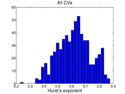
In Fig. (1) is shown the histogram of the Hurst exponents of all the CVs analyzed by Fritz and Bruch. We see that both persistent and antipersistent behaviors are present. We note that the peak is around $H\sim 0.65$. At the value $H\sim 0.73$ found by Hurst in most natural phenomena there is a drastic drop. The presence of a second bump at $H\sim 0.82$ is also possible. We then notice that the distribution is non symmetric with a longer tail towards the shorter values of $H$.

Figure 1: Histogram of the Hurst exponent of all the sample of CVs. The distribution peaks at $H\simeq 0.65$. Around the value found by Hurst for most of the natural phenomena $H\sim 0.73$ there is instead a drop in the distribution. The presence of a second bump at $H\sim 0.82$ is also possible. The distribution is non symmetric showing a tail towards the shorter values of $H$.

3 The flickering in white light of V709 Cas

V709 Cas (RX J0028.8+5917) is a DQ Her–type system with orbital period of 0.2225 days bonnetbidaud2001 and a $1.08M_{\odot}$ primary (Ramsay, (2000)) with a spin period $P_{spin}=312.8$ s (De Martino et al., (2001)). We have analyzed six runs obtained in white light during a multi–site photometric campaign performed from September 22 to October 2 2000 by De Martino et al. (2002) with a three channel photometer placed at the 0.8 m Tenerife (Spain), at the 1.5 m Loiano (Italy) and at the 0.8m Beijing (China) telescopes. The integration time was in all cases 10s.

The lightcurves (Fig. 2-3) show very rapid variations up to 0.2 magnitudes, indicating the presence of a strong flickering, as already reported by Kozhevnikov (2001) and De Martino et al. (2002).

Figure 2: The full set of the original and the “corrected lightcurves” of V709 Cas (see text). The last night of observations has been omitted in the right panel because of the presence of low quality data.

Figure 3: The corrected lightcurves of the six runs (a–f) of Tab.1. Time is in days and magnitudes are rescaled with respect to their mean magnitude. The discontinuities in the last two datasets are due to the presence of veils during the observations.

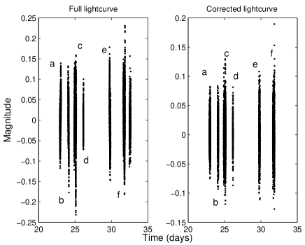
Each inset of Fig. 3 shows the “corrected lightcurve”, i.e. the lightcurve variations with the magnitude rescaled with respect to zero and filtered from the fluctuations due to the orbital period of the CV. The data sets are ordered as in Table 1. From up to down the first subplot (a), shows, with respect to the other subsets of data, a more active flickering, with more erratic motions, rapid and intense flares. The third and fifth subplot (c) and (f) show a larger variance at shorter timescales and shorter variance at larger timescales. They both present flares with larger amplitudes up to 0.2 mag.

Figure 4: The power spectra of the six corrected lightcurves of V709 Cas.

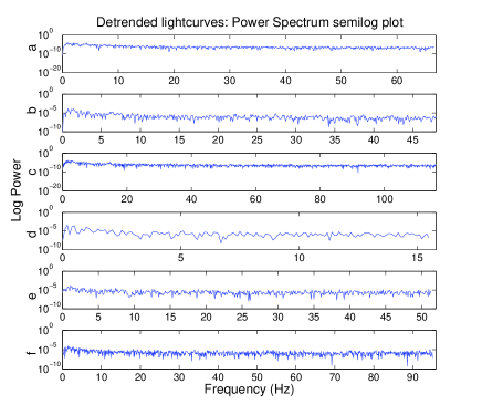
The power spectra of the corrected lightcurves do not show any dominating periodicity (Fig. 4). The presence of some residual power ($\sim 10^{-4}$) is present at low frequencies, but it will not appreciably affect the results of our analysis.

3.1 Data analysis

Now we determine the parameter $\alpha$ both with wavelets and Hurst R/S analysis and plot for each run the position of V709 Cas in the parameter space $\alpha$-$\Sigma$ with the time scale resolution of 10 seconds. We used the C12 wavelets (Fritz & Bruch, 1998). To test our software we used both wavelet-generated FBMs and $1/f^{\beta}$ Gaussian processes (Bak et al., 1987; Abry et al., 1995). Each lightcurve (a–f) was divided into series of $2^{n}$ bins, with $n$ is an integer varying in the interval $[1,7]$ in order to apply the prescriptions of wavelet analysis.

Tab. 1 gives, for each run, the Hurst exponent $H$ and the characteristic exponent $\beta$ of the $1/f^{\beta}$ process obtained with wavelets. The table also reports the run label, the number of data points, the maximum and minimum of the relative magnitudes, and the percentage difference $\Delta\%=\frac{|D_{H}-D_{f}|}{|D_{H}+D_{f}|}\times 100$ between the the fractal exponent $D$ calculated with the $1/f^{\beta}$ noises ($D_{f}=1+\frac{\beta}{2}$) and with the R/S analysis ($D_{H}=2-H$).

The Hurst exponents of each of the six acquisitions reported in Tab 1 are all larger than $1/2$, indicating that the flickering of V709 Cas is always is a stochastic process with persistent memory in time. The averaged value of $H$ is $0.63$ and the standard deviation is $0.05$. The value obtained, with R/S the analysis, reported in the table, fluctuates between $H=0.58$ and $H=0.72$. However, the differences $\Delta\%$ are rather small.

Table 1:

Run	data	Max	min	$\beta$	H	$\Delta\%$
a	1335	0.082	-0.075	0.82	0.59	1.2
b	974	0.084	-0.093	0.72	0.64	8.3
c	2325	0.130	-0.119	0.80	0.60	3.8
d	312	0.081	-0.087	0.56	0.72	4.3
e	1029	0.108	-0.111	0.72	0.64	4.2
f	1904	0.190	-0.127	0.82	0.59	7.3

Fig. 5 presents the scalegrams for the six corrected lightcurves, i.e. the log-log plot of the variance $S(t_{s})$ vs. the chosen time scale $t_{s}$.

Figure 5: Scalegrams of the six acquisitions of the corrected V709 Cas data. The lines corresponding to different acquisitions are quite similar showing a stability of $\alpha$ during 10 days. The small differences at short time scales may be due to different Poisson noise contributions.

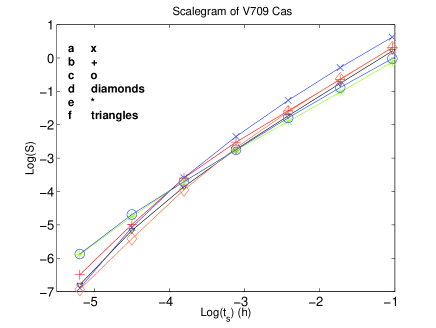
The curves rise linearly with the time intervals and remain quite linear for all the 6 acquisitions. This suggests that the flickering remains self–similar, with the same power–law exponent, from the tens of minutes down to the $10$ second time scale. We also see that all the curves almost overlap yielding a quite stable value of $\alpha$, indicating that, during the 10 days-period of observations, the flickering and the accretion process of the CV remained quite stable.

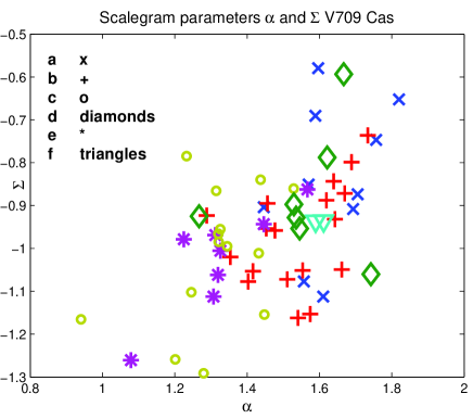
Fig. 6 shows all the values of $\alpha$ and $\Sigma$ of V709 Cas. The values span in the interval $0.9<\alpha<1.8$ and $-1.3<\Sigma<-0.6$, typical of magnetic CVs (Bruch, (1992)). In the ($\alpha,\Sigma$) plane the values obtained from V709 Cas show a trend. $\Sigma$ is shown to decrease with decreasing $\alpha$. This would suggest that the persistence character of the light fluctuations and the energies implied are anticorrelated.

Figure 6: The $\alpha$–$\Sigma$ parameter space for all the V709 Cas data. All the values for each wavelet octave are reported. The relatively small region of the diagram occupied by the data indicates a rather stable stochastic phenomenon.

4 Conclusions

We have analyzed the flickering observed in six optical photometric runs of the IP V709 Cas. In their pioneering work, Fritz and Bruch (1998), tried to correlate the characteristics of the flickering of CVs with their subtypes using wavelet analysis and the scalegram. The stochastic properties of flickering were described by using the two parameter space $\alpha$-$\Sigma$. In this paper the parameter $\alpha$ was obtained both with the wavelets and the Hurst R/S analysis, the latter being a statistical robust method. During the 10 days of the observations the stochastic properties of the flickering did not change indicating that the physics of the accretion process remained relatively stable. We also noticed that the values of $\alpha$ and $\Sigma$ parameters, calculated at different epochs and at different time scales, show a trend suggesting that the persistence character of the light fluctuations and the energies implied in the accretion process are anticorrelated. In the ($\alpha$, $\Sigma$) diagram V709 Cas falls in the region of magnetic systems. However, this CV was recognized as an IP only from its X-ray lightcurve while no spin modulation in the optical range is observed and the lightcurve is strongly flickering–dominated without any precise and stable dominating frequency, with the exception made for frequencies related to the orbital motion. Therefore, V709 Cas may represent an ideal test case where the $\alpha-\Sigma$ classification improved by the Hurst R/S analysis can be used to characterize CV subtypes, especially when the classification is uncertain.

Hurst’s R/S analysis can also provide a useful tool for understanding the results of high speed photometry. In particular, it could give precious information to show down to which short time–scale the flickering can be still considered self–similar, revealing the physics behind very short time scale phenomena. Thus, a futuristic application might be suggested for ultra-fast photometry towards the quantum limit (Dravins et al., (2005)).

5 Acknowledgments

One of us, FT, also gratefully acknowledges the financial support from the CARIPARO Foundation inside the 2006 Program of Excellence. DdM and AB acknowledge financial support from INAF PRIN N.17.

References

- Abry et al., (1995) Abry, P., Gonçalvès, P., and Flandrin, P., in ” Lecture Notes in Statistics”, 103. Wavelets and Statistics. A. Antoniadis, G. Oppenheim (Editors) Springer-Verlag, 1995.
- Bak et al., (1987) Bak, P., Tang, C. and Wiesenfeld, K., 1987, Phys. Rev. Lett., 59, 381.
- Bruch, (1992) Bruch A., 1992, A&A 266, 237.
- (4) Bruch A., 1992, in Viña del Mar Workshop on Cataclysmic Variable Stars ASP conference series 29, ed. N. Vogt.
- Bruch, (1995) Bruch A., 1992 in: J. Greiner et al. , eds., ”Flares and Flashes”, Proc. IAU Coll. 151, Springer Verlag, Heidelberg, p. 288.
- Bruch, (1996) Bruch, A. 1996, A&A, 312, 97.
- Bruch and Grutter, (1997) Bruch, A., and Grutter, M., Acta Astronomica, 47, 307, 1997.
- Chui, (1992) Chui C.K., 1992, An Introduction to Wavelets, Academic Press Inc., San Diego.
- De Martino et al., (2001) De Martino, D., Matt, G., Mukai, K., Belloni, T., Bonnet-Bidaud, J.M., Chiappetti, L., Gaensicke, B.T., Haberl, F. and Mouchet, M., A&A 377, 499-511, (2001).
- De Martino et al., (2002) De Martino, D., et al. ASPC 261, 145 (2002).
- Dravins et al., (2005) Dravins D., Barbieri C., Da Deppo V., Faria D., Fornasier S., Fosbury R.A.E., Lindegren L., Naletto G., Nilsson R., Occhipinti T., Tamburini F., Uthas H., Zampieri L. 2005, ”QuantEYE. Quantum Optics Instrumentation for Astronomy” OWL Instrument Concept Study, ESO document OWL-CSR-ESO-00000-0162 (2005).
- Elsworth & James, (1982) Elsworth, Y. P. & James, J. F., 1982, MNRAS 198, 889.
- Elsworth & James, (1986) Elsworth, Y. P. & James, J. F., 1986, MNRAS 220, 895.
- Feder, (1988) Feder, J., 1988, Fractals, Plenum Press, NY.
- Fritz & Bruch, (1998) Fritz, T. and Bruch, A., 1998, A&A, 332, 586.
- Gammel, (1997) Gammel, B. M., 1997, Phys. Rev. E, 58, 2, 2586.
- Gao et al., (2003) Gao, J. B., Yinhe Cao and Lee. J.–M., 2003, Phys. Lett. A, 314, 392.
- Gill & Henriksen, (1990) Gill, A. G., & Henriksen, R. N., 1990, ApJ, 365, L27–L30.
- Haberl & Motch (1995) Haberl F., Motch C., 1995, A&A 297, L37.
- Hanslmeier et al., (2000) Hanslmeier, A., Kucera, A., Rybák, J., Neunteufel, B. and Wöhl, H, A&A, 356, 308, 2000.
- Hurst, (1951) Hurst, H. E., Trans. Am. Soc. Civ. Eng. 116, 770, 1951.
- Hurst et al., (1965) Hurst, H. E., Black, R. and Sinaika, Y. M., Long-Term Storage in Reservoirs: An Experimental Study (Constable, London, 1965).
- James, (1987) James, J. F., 1987, MNRAS, 224, 227.
- Kozhevnikov, (2001) Kozhevnikov V. P., 2001, A&A 366, 891.
- Livio, (1992) Livio M., 1992, ApJ 393, 516.
- Lowen, (1999) Lowen, S. B., 1999, Methodology and Computing in Applied Probability 1, 4, 445-456, Springer Netherlands ISSN 1387-5841 (Print) 1573-7713 (Online)
- Mandelbrot & van Ness, (1968) Mandelbrot, B. B. & van Ness, 1968, SIAM (Soc. Ind. Appl. Math.) Rev. 10, 422.
- Mandelbrot & Wallis, (1969) Mandelbrot, B. and Wallis, J.: 1969, Water Resources Res. 5, 321.
- Moffet & Barnes, (1974) Moffett, T. J., & Barnes, T. G., 1974, ApJ, 194, 141.
- Mumford, (1966) Mumford, G. S., 1966, ApJ, 146, 411.
- Norton et al., (1999) Norton, A. J., Beardmore, A. P., Allan, A., and Hellier, C. 1999, A&A, 347, 203.
- Oliver & Ballester, (1998) Oliver, R. & Ballester, J. L., 1998, Phys. Rev. E, 58, 5, 5650.
- Percival & Walden, (2000) Percival, D. B. and Walden, A. T., 2000, Wavelet Methods for Time Series Analysis, Cambridge University Press
- Ramsay, (2000) Ramsay, G., 2000, MNRAS 314, 403.
- Robinson, (1973) Robinson, E. L., 1973, ApJ, 180, 121; ApJ, 181, 531; ApJ, 183, 193.
- Scargle et al., (1993) Scargle J.D., Steinman-Cameron T.Y., Young K., Donoho D.L., Crutch- field J.P., Imamura J., 1993, ApJ 411, L91.
- Simonsen et al., (1998) Simonsen, I., Hansen, A. and Magnar Nes, O., 1998, Phys. Rev. E, 58, 2779.
- van Amerongen et al., (1987) van Amerongen, S., Damen, E., Groot, M., Kraakman, H. and van Paradijs, J., 1987, MNRAS 225, 93.
- Warner & O’Donoghue, (1987) Warner, B., & O’Donoghue , D., 1987, MNRAS, 224, 733.
- Warner & Nather, (1971) Warner, B., & Nather, R. E., 1971, MNRAS, 152, 219.
- Warner, (1975) Warner, B., 1975, MNRAS, 170, 219.
- Warner, (1995) Warner B., 1995, Cataclysmic Variable Stars, Cambridge University Press.
- Woudt & Warner (2001) Woudt, P. A. and Warner, B., 2001 MNRAS, 328, 159.
- Woudt & Warner (2002) Woudt, P. A. and Warner, B., 2002, MNRAS, 335, 44.
- (45) Woudt, P. A. and Warner, B., 2002, Ap&SS, 282, 433
- Woudt & Warner (2003) Woudt, P. A. and Warner, B., 2003, MNRAS, 339,731
- (47) Woudt, P. A. and Warner, B., 2003, MNRAS, 340, 1011
- Woudt et al. (2004) Woudt, P. A., Warner, B. and Pretorius, M. L., 2004, MNRAS 351, 1015.
- Woudl et al. (2005) Woudt, P. A., Warner, B. and Spark, M., 2005, MNRAS 364, 107.
- Woudt & Warner (2008) Woudt, P. A. and Warner, B., 2008, arXiv:0806.1317v1 [astro-ph], to appear in “Cool discs, hot flows: The varying faces of accreting compact objects” (AIP Conf. Series), 2008.
- Zamanov & Bruch, (1998) Zamanov, R. Z. & Bruch, A., 1998, A&A, 338, 988.
- Zuckermann, (1971) Zuckermann, M. –C., 1961, Ann. d’Astrophys. 24, 431.