A Tight Estimate for Decoding Error-Probability of LT Codes Using Kovalenko’s Rank Distribution

Abstract

A new approach for estimating the Decoding Error-Probability (DEP) of LT codes with dense rows is derived by using the conditional Kovalenko’s rank distribution. The estimate by the proposed approach is very close to the DEP approximated by Gaussian Elimination, and is significantly less complex. As a key application, we utilize the estimates for obtaining optimal LT codes with dense rows, whose DEP is very close to the Kovalenko’s Full-Rank Limit within a desired error-bound. Experimental evidences which show the viability of the estimates are also provided.

I Introduction and Backgrounds

For Binary Erasure Channels (BEC), the task of a Luby Transform (LT) decoder is to recover the unique solution of a consistent linear system

$$HX^{T}=\beta^{T},\quad\beta=(\beta_{1},\dots,\beta_{m})\in(\mathbb{F}_{2}^{s})^{m},$$ (I.1)

where $H$ is an $m\times n$ matrix over $\mathbb{F}_{2}$. This can be explained briefly as follows. (For detailed backgrounds, see [1, 2, 3]). In LT codes, to communicate an information symbol vector $\alpha=(\alpha_{1},\dots,\alpha_{n})\in(\mathbb{F}_{2}^{s})^{n}$, a sender constantly generates and transmits a syndrome symbol $\beta_{i}=H_{i}\alpha^{T}$ over BEC, where $H_{i}\in\mathbb{F}_{2}^{n}$ is generated uniformly at random on the fly by using the Robust Soliton Distribution (RSD) $\mu(x)$ [1]. A receiver then acquires a set of pairs $\{(H_{i_{t}},\beta_{i_{t}})\}_{t=1}^{m}$ and interprets it as system (I.1), and hence, the variable vector $X=(x_{1},\dots,x_{n})\in(\mathbb{F}_{2}^{s})^{n}$ represents the information symbol vector $\alpha$. Unlike LDPC codes, the row-dimension $m$ of $H$ is a variable and the column-dimension $n$ is fixed. Thus a reception overhead defined as $\gamma=\frac{m-n}{n}$ is the key parameter for measuring error-performance of LT codes.

System (I.1) has the unique solution $X=\alpha$ iff $\text{Rank}(H)=n$, the full rank of $H$. In case of the full-rank, $\alpha$ can be recovered by using a Maximum-Likelihood Decoding Algorithm (MLDA) such as the ones in [5, 15]. These algorithms are an efficient Gaussian Elimination (GE) that fully utilize an approximate lower triangulation of $H$, obtainable by exploiting the diagonal extension process with various greedy algorithms in [4, 5, 6, 15]. Under those GE, thus, the probability of decoding success is the full-rank probability $\Pr(\text{Rank}(H)=n)$.

It is shown in [1] by Luby that, when $H$ is generated by the RSD with large $n$ and $\gamma\geq\ln(n/\delta)/\sqrt{n}$, system (I.1) can be solved for $X=\alpha$ by using the Message Passing Algorithm (MPA) in [7] with the minimum probability $1-\delta$, and the number of row operations to compute $X=\alpha$ by the MPA is $O(n\ln(n/\delta))$. For short $n$, however, a stable overhead $\gamma$ needed for successful decoding by the MPA with high probability is not trivial. In fact, even under GE that is much superior to the MPA in error-performance, a stable $\gamma$ to achieve the full-rank probability near one is not trivial.

Let $H$ of system (I.1) be an $m\times n$ binary random matrix generated by a row-degree distribution $\rho(x)=\sum\rho_{d}x^{d}$ with $m=(1+\gamma)n$. The Decoding Error Probability (DEP) of an LT code generated by $\rho(x)$ used in this paper is the rank-deficient probability defined as

$$\text{P}_{\text{err}}^{\text{ge}}(1+\gamma,n,\rho) = 1-\Pr(\text{Rank}(H)=n)$$ (I.2)

$$= \Pr(\text{Rank}(H)<n).$$ (I.3)

Then with a desired error-bound $\delta\in(0,1)$, define

$$\gamma_{\min}(\delta,n,\rho)=\min_{\gamma\geq 0}\{\gamma\>|\>\text{P}_{\text{err}}^{\text{ge}}(1+\gamma,n,\rho)\leq\delta\},$$ (I.4)

and refer to as the Minimum Stable Overhead (MSO) of the code with $\delta$. With $m=(1+\gamma)n$ symbols of $\beta$ where $\gamma\geq\gamma_{\min}(\delta,n,\rho)$, thus, the recovery of $\alpha$ can be accomplished by GE decoding with probability at least $1-\delta$.

It was shown in [14] that probabilistic lower-bounds for DEP and MSO of random binary codes exist, called Kovalenko’s Full-Rank Limit and Overhead (KFRL and KFRO respectively). Specifically, KFRL is the function

$$K(1+\gamma,n)=1-\prod_{i=k+1}^{n}\left(1-\frac{1}{2^{i}}\right),\quad k=\gamma n,$$ (I.5)

where $K(1+\gamma,n)\leq\text{P}_{\text{err}}^{\text{ge}}(1+\gamma,n,\rho)$. Hence, the DEP of LT and LDPC codes cannot be lower than KFRL. Similar to MSO, KFRO is the minimum $\gamma$ defined as

$$\gamma_{K}(\delta,n)=\min_{\gamma}\{\gamma\geq 0\>|\>K(1+\gamma,n)\leq\delta\},$$ (I.6)

where $\gamma_{K}(\delta,n)\leq\gamma_{\min}(\delta,n,\rho)$. For successful decoding under the constraint $\text{P}_{\text{err}}^{\text{ge}}(1+\gamma,n,\rho)\leq\delta$, thus, the minimum number of symbols of $\beta$ that a receiver should acquire is at least $(1+\gamma_{K}(\delta,n))n$ [14, Theorem 2.2]. For short $n$ and small $\delta$, since the KFRO $\gamma_{K}(\delta,n)$ is not trivial, the MSO $\gamma_{\min}(\delta,n,\rho)$ is not trivial. It was also observed experimentally that $K(1+\gamma,n)\approx 2^{-\gamma n}$ as $\gamma$ increases. For small $\delta$, therefore, $\gamma_{K}(\delta,n)\approx\frac{k_{\delta}}{n}$, where $k_{\delta}=\min\{k\in\mathbb{N}^{+}\;|\;2^{-k}<\delta\}$.

Let $\mu(x)=\sum_{d\leq d_{0}}\mu_{d}x^{d}$, a truncated form of RSD where $\lim_{n\to\infty}\frac{d_{0}}{n}=0$. For short $n$, the DEP of codes (generated) by a truncated $\mu(x)$ alone exhibits error-floors over a large range of $\gamma$. The error-floor region however can be lowered to near zero dramatically by supplementing a small fraction of dense rows to $\mu(x)$ (see [12, 13, 14]). The row-degree distribution $\rho(x)$ considered in this paper is thus a supplementation of $\mu(x)$ with a fraction of rows of degree $\frac{n}{2}$ as shown below

$$\rho(x)=\sum_{d\leq d_{0}}\left(\frac{\mu_{d}}{1+\kappa}\right)x^{d}+\left(\frac{\kappa}{1+\kappa}\right)x^{n/2},\quad\kappa\geq 0.$$ (I.7)

By rearranging rows, an $H$ by $\rho(x)$ above can be expressed as $H=\left[\begin{smallmatrix}\tilde{H}\\ \hat{H}\end{smallmatrix}\right]$, where $\tilde{H}$ is a sparse matrix generated by $\mu(x)$ and $\hat{H}$ is a dense one formed by random rows of degree $\frac{n}{2}$. The key objective of optimizing LT codes in this paper is to obtain a $\rho(x)$, by which, generated LT codes can achieve the $\gamma_{\min}(\delta,n,\rho)$ near the $\gamma_{K}(\delta,n)$ for better error-performance, but the dense fraction $\rho_{n/2}=\frac{\kappa}{1+\kappa}$ is as small as possible for encoding and decoding efficiency.

In the paper [15], a simple way of using an Upper-Bound of DEP (UBDEP) was formulated for the fast optimization. This approach was quite effective in that, an estimate of the UBDEP by the formulation is close to the DEP approximated by GE and is obtainable very rapidly (within a fraction of a second using a standard computer). Hence, the optimization was accomplished very rapidly as well by checking the estimates with various fractions for $\rho_{n/2}$.

In this paper, an exact formulation of DEP is derived by decomposing the full-rank probability in (I.2) as a sum of conditional full-rank probabilities, that are computable quite rapidly by using by the conditional Kovalenko’s rank-distribution. The formulation is similar to that of UBDEP in that, it uses prior knowledges of the rank-distribution of the sparse part $\tilde{H}$. The Estimate of DEP (EDEP) by the formulation is however extremely close to the DEP approximated by GE, and also is computable quite rapidly (again, within a fraction of a second on a standard computer). Thus, a finer optimization of $\rho(x)$ can be accomplished very fast by checking EDEP’s with various fractions for $\rho_{n/2}$.

The remainder of this paper is organized as follows. In Section II, a simple approach for generating a truncated RSD for a supplementation $\rho(x)$ in (I.7) is presented. In Section III, explicit formulations of DEP and UBDEP are derived by analyzing the full-rank probability in (I.2) and the rank-deficient probability in (I.3), respectively, and are utilized for obtaining an optimal $\rho(x)$. The KFRL in (I.5) is also explained by the conditional Kovalenko’s rank-distribution in this section. In Section IV, further experimental results which show the viability of the EDEP are presented. This paper is summarized in Section V.

II A Truncation of an RSD

The RSD considered for the truncation in (I.7) is the one in [3, Ex.50.2]. Let $h(d)$ denote the expected number of rows of degree $d$ of an $H$ by $\mu(x)$. With $S\geq 1$, we have

$$h(d)=\begin{cases}S+1,&\text{if }d=1\\ \frac{n}{d(d-1)}+\frac{S}{d},&\text{otherwise}\end{cases}.$$ (II.1)

Setting the number of rows of $H$ as

$$m=\sum_{d=1}^{n}h(d)\approx n+S(1+\ln(n)),$$ (II.2)

then normalizing $h(d)$ by the $m$ yields

$$\mu(x)=\sum_{d=1}^{n}\mu_{d}x^{d},\quad\text{where}\quad\mu_{d}=\frac{h(d)}{m}.$$ (II.3)

For more detail, see [15, Section-IV].

Consider now a truncated RSD in such a way that $\mu(x)=\sum_{d\leq d_{0}}\mu_{d}x^{d}$, where $\lim_{n\to\infty}\frac{d_{0}}{n}=0$. Let $H$ be now an $m\times n$ matrix generated by a truncated $\mu(x)$. The reason behind this truncation is that in practice, most of the fractions of the $\mu(x)$ in (II.3) are too small to get $m\mu_{d}\geq 1$. Fractions for higher degrees however should be assigned appropriately to meet the constraint on the density (in number of nonzero entries of $H$),

$$a_{r}=\sum_{d\leq d_{0}}d\cdot\mu_{d}\quad\geq\quad\frac{\ln(n/\epsilon)}{(1+\gamma)},$$ (II.4)

where $a_{r}$ is the average row-degree of $H$. By doing so, all columns of $H$ of system (I.1) are nonzero with probability at least $1-\epsilon$. This constraint can be explained by looking at the column-degree distribution of $H$,

$$\lambda(x)=\prod_{d=1}^{d_{0}}\left[\left(1-\frac{d}{n}\right)+\left(\frac{d}{n}\right)x\right]^{(1+\gamma)n\mu_{d}},$$ (II.5)

as follows. From $\lambda(x)$, we have $n\lambda(0)\approx ne^{-(1+\gamma)a_{r}}$ as the expected number of null columns of $H$. With an appropriate $d_{0}$, therefore, fractions of $\mu(x)$ should be assigned to meet the inequality $ne^{-(1+\gamma)a_{r}}\leq\epsilon<1$, that is equivalent to (II.4).

For short $n$, even if a truncated $\mu(x)$ meets the constraint (II.4), experiments exhibited that the DEP of codes by $\mu(x)$ alone exhibits error-floors over a large range of $\gamma$. A desirable feature of $\mu(x)$ is however that, for $\gamma\geq 0$, the DEP is mainly contributed by the rank-deficient probabilities $\Pr(\text{Rank}(H)=n-\eta)$ of small $\eta$. In Fig. III.1, for example, the curve $\text{P}_{\text{err}}^{\text{ge}}(1+\gamma,100,\mu)$, where $\mu(x)$ is a truncated one in table III.1, is the DEP approximated by the GE in [15] called the Separated MLDA (S-MLDA). As can be seen clearly, it never reaches the bound $\delta=10^{-3}$ for $1+\gamma\leq 1.3$. As $\gamma$ increases, on the other hand, it is very close to the deficiency curve $\eta=1$ and is almost identical to the sum of deficiency probabilities of $\eta=1,\dots,7$. These deficiency probabilities can be lowered to near zero dramatically when enough number of dense rows are supplemented to $H$. The portion of the density increased by the dense rows alone however could be much larger than expected. Therefore, with a desired $\delta$, the fraction for $\rho_{n/2}$ of $\rho(x)$ in (I.7) should be as small as possible, while maintaining the $\gamma_{\min}(\delta,n,\rho)$ near the $\gamma_{K}(\delta,n)$.

Let $\mathcal{D}_{1}=\{1,2,\dots,d_{s}\}$, and let $\mathcal{D}_{2}$ be a set of few spike degrees $d$ such that $d_{s}<d\leq d_{0}$ for some $d_{0}$. A truncation of $\mu(x)$ is summarized as follows.

1. Generate the $\mu(x)$ in (II.3) with desired $S$, $n$, and $\epsilon$.

2. Take a few spike terms for $\mathcal{D}_{2}$, if necessary, such that $\sum_{d\in\mathcal{D}_{2}}\mu_{d}=1-\sum_{d\in\mathcal{D}_{1}}\mu_{d}$, and at the same time to hold $a_{r}\geq\frac{\ln(n/\epsilon)}{1+\gamma}$ as in (II.4).

Thus, hopefully, columns of $H$ by a truncated $\mu(x)$ have a one in some rows of degree $d\in\mathcal{D}_{1}\cup\mathcal{D}_{2}$ with probability at least $1-\epsilon$. An exemplary $\mu(x)$ generated by R1 and R2 is listed in table III.1, and its supplementation $\rho(x)$ with various fractions for $\rho_{n/2}$ was used for computer simulations presented in Fig. III.2 and Fig. IV.1.

III The Proposed Estimate for DEP of LT Codes

We first introduce the optimization of $\rho(x)$ in [15] that uses estimated UBDEP’s. Let $H$ of system (I.1) be generated by a supplementation $\rho(x)$ in (I.7) with $m=(1+\gamma)n$. By rearranging rows, we have $H=\left[\begin{smallmatrix}\tilde{H}\\ \hat{H}\end{smallmatrix}\right]$, where the sparse part $\tilde{H}$ is generated by a truncated $\mu(x)$ and the dense part $\hat{H}$ is formed by random rows of degree $\frac{n}{2}$. Let $B(m,k,p)=\binom{m}{k}p^{k}(1-p)^{m-k}$ be the Bernouli probability with $0\leq p\leq 1$. Assume that the dense part $\hat{H}$ attains $k$ rows with probability $B(m,k,\rho_{n/2})$. With the sparse part $\tilde{H}$, let $\varphi_{\mu}(\eta)=\Pr(\text{Rank}(\tilde{H})=n-\eta)$. Let $\vartheta_{\rho}(k,\eta)=\Pr(\text{Rank}(H)<n|k,\eta)$ the conditional probability that $\text{Rank}(H)<n$, given that $\hat{H}$ attained $k$ rows and $\text{Rank}(\tilde{H})=n-\eta$. Finally, let $\vartheta_{\rho}(k)=\Pr(\text{Rank}(H)<n|k)$ the conditional probability that $\text{Rank}(H)<n$ given that $\hat{H}$ attained $k$ rows. We have $\vartheta_{\rho}(k)=\sum_{\eta=1}^{n}\vartheta_{\rho}(k,\eta)\cdot\varphi_{\mu}(\eta)$.

The UBDEP in [15] was formulated in two steps: first by expressing the DEP in (I.3) as the sum

$$\text{P}_{\text{err}}^{\text{ge}}(1+\gamma,n,\rho)=\sum_{k=0}^{m}B(m,k,\rho_{n/2})\cdot\vartheta_{\rho}(k),$$ (III.1)

second, by finding an upper-bound for $\vartheta_{\rho}(k)$ as shown in the following theorem. (For the proof, see [15, Theorem IV]).

Theorem III.1 (The UBDEP of LT codes by $\rho(x)$).

Since $\vartheta_{\rho}(k,\eta)\leq\frac{1}{2^{k-\eta}}$ for $1\leq\eta\leq k$ by the union bound and $\vartheta_{\rho}(k,\eta)=1$ for $\eta>k$, we have

$$\vartheta_{\rho}(k)\leq\left(\overline{\vartheta_{\rho}(k)}=\sum_{\eta=1}^{k}\frac{\varphi_{\mu}(\eta)}{2^{k-\eta}}+\sum_{\eta>k}\varphi_{\mu}(\eta)\right).$$ (III.2)

This yields the UBDEP as shown below

$$\text{P}_{\text{err}}^{\text{ge}}(1+\gamma,n,\rho)\leq\sum_{k=0}^{m}B(m,k,\rho_{n/2})\cdot\overline{\vartheta_{\rho}(k)}.$$ (III.3)

Notice that, once the deficient probabilities $\phi_{\mu}(\eta)$, $\eta=1,2,\dots,\eta_{0}$, are estimated for some $\eta_{0}$ (e.g., the deficiency curves $\eta=1,2,\dots,27$ in Fig. III.1), the UBDEP in (III.3) can be estimated very fast for any fraction for $\rho_{n/2}$. Furthermore, experiments exhibited that the estimate is also close to the DEP approximated by GE over system (I.1). Thus the overall shape of DEP including its error-floor region is predictable from the estimates right away. Exemplary optimizations using these estimates are presented in [15].

We shall now decompose the $\Pr(\text{Rank}(H)=n)$ in (I.2) as a sum of conditional full-rank probabilities of $H$. Let us clarify some notations first. With $0\leq\omega\leq\min\{k,\eta\}$, let

$$\zeta(\eta,\omega,k)=\Pr(\text{Rank}(H)=(n-\eta)+\omega|\eta,k),$$ (III.4)

the conditional probability that $\text{Rank}(H)=(n-\eta)+\omega$ given that $\text{Rank}(\tilde{H})=n-\eta$ and $\hat{H}$ attained $k$ rows. Assume that the dense part $\hat{H}$ attains $k$ rows with probability $B(m,k,\rho_{n/2})$. Let $\Pr(\text{Rank}(H)=n|k)$ denote the conditional full-rank probability given that $\hat{H}$ attained $k$ rows. We have, first,

$$\Pr(\text{Rank}(H)=n|k)=\sum_{\eta=0}^{k}\zeta(\eta,\eta,k)\phi_{\mu}(\eta),$$ (III.5)

where $\phi_{\mu}(\eta)=\Pr(\text{Rank}(\tilde{H})=n-\eta)$. Second,

$$\Pr(\text{Rank}(H)=n) = \sum_{k=0}^{m}B(m,k,\rho_{n/2})$$ (III.6)

$$\;\cdot\Pr(\text{Rank}(H)=n|k).$$

Then finally, we have

$$\text{P}_{\text{err}}^{\text{ge}}(1+\gamma,n,\rho)=1-(\text{\ref{eq:frp0}}).$$ (III.7)

An explicit formulation of $\zeta(\eta,\omega,k)$ in (III.5) is possible by interpreting Kovalenko’s rank-distribution [8, 9, 10, 11, 13] as the conditional one as shown in the following lemma.

Lemma III.1 (The Conditional Kovalenko’s Rank-Distribution).

For any $(\eta,\omega,k)$ with $\omega\leq\min\{\eta,k\}$, we have

$$\zeta(\eta,\omega,k)=\frac{S(\omega,l)}{2^{l(\eta-\omega)}}\prod_{i=1}^{\omega}\left(1-\frac{1}{2^{\eta+1-i}}\right),$$ (III.8)

where, with $l=k-\omega$,

$$S(\omega,l)=\sum_{i_{1}=0}^{\omega}\sum_{i_{2}=i_{1}}^{\omega}\cdots\sum_{i_{l}=i_{l-1}}^{\omega}\frac{1}{2^{i_{1}+\cdots+i_{l}}},$$ (III.9)

holding the recursion

$$S(\omega,l)=\frac{1}{2^{l}}S(\omega-1,l)+S(\omega,l-1).$$ (III.10)

Proof:

The proof can be accomplished inductively by using the recursions (III.10) and

$$\zeta(\eta,\omega,k+1) = \zeta(\eta,\omega-1,k)\left(1-\frac{1}{2^{\eta-\omega+1}}\right)$$ (III.11)

$$+\quad\zeta(\eta,\omega,k)\frac{1}{2^{\eta-\omega}}.$$

For detailed proof, we refer readers to [13, Lemma IV.3]. ∎

	$(\mu_{d})_{d=1}^{5}=(0.014,0.481,0.152,0.082,0.048)$
$\mathcal{D}_{1}$	$(\mu_{d})_{d=6}^{10}=(0.034,0.024,0.024,0.012,0.012)$
$\mathcal{D}_{2}$	$\mu_{25}=0.059$, $\mu_{35}=0.058$

TABLE III.1: Fractions of $\mu(x)$ generated by the steps R1) and R2) with $S=10$ and $n=10^{3}$.

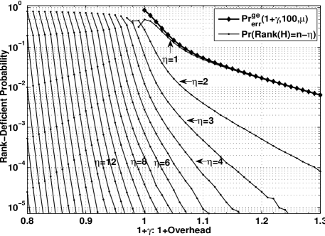
Figure III.1: The curves $\eta=1,2,\dots,$ represent $\phi_{\mu}(\eta)=\Pr(\text{Rank}(\tilde{H})=n-\eta)$ approximated by the S-MLDA, where $\tilde{H}$ is generated by the $\mu(x)$ in table III.1 with $n=100$.

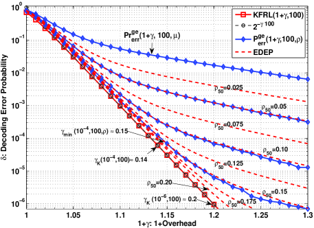
Figure III.2: In the figure, $\rho(x)$ is a supplementation of the $\mu(x)$ in table III.1 with an assigned dense fraction for $\rho_{n/2}$. For each fraction for $\rho_{n/2}$, the DEP curve is approximated by the S-MLDA and the EDEP is computed by using the finite version in (III.12).

Theorem III.2.

Assume that $\phi_{\mu}(\eta)$ in (III.5) are explicitly known over a deficiency range $1\leq\eta\leq\eta_{0}$ for some $\eta_{0}$. Then the DEP in (III.7) is explicitly computable.

Proof:

Since $\zeta(\eta,\omega,k)$ in (III.4) is explicitly computable by the recursions (III.10) and (III.11), $\zeta(\eta,\eta,k)$ in (III.5) is computable by $S(\eta,k-\eta)\prod_{i=1}^{\eta}(1-2^{-i})$. Therefore, the DEP in (III.7) is explicitly computable. ∎

The DEP in (III.7) is very practical in two respects. First, for any fraction for $\rho_{n/2}$, experiments exhibited that the EDEP is almost identical to the DEP approximated by GE. Second, the full-rank probability in (III.6) can be estimated very rapidly, and therefore, a fine optimization of $\rho(x)$ is obtainable very fast by checking EDEP’s with various fractions for $\rho_{n/2}$. The following example shows the viability that the EDEP is very close to the DEP approximated by the S-MLDA over system (I.1). An exemplary optimization of $\rho(x)$ using EDEP’s is also presented in the example.

Example III.1.

In Fig. III.1, the deficiency curves $\eta=1,2,3,\dots,27$, represent $\phi_{\mu}(\eta)=\Pr(\text{Rank}(\tilde{H})=n-\eta)$ approximated by the S-MLDA over system (I.1). In Fig. III.2, blue curves are DEP’s approximated by the S-MLDA, where $\rho(x)$ is a supplementation of the $\mu(x)$ in table III.1 with a dense fraction in $\rho_{n/2}=\{0.05,0.10,0.15\}$, and dashed curves in red are EDEP’s of codes by $\rho(x)$ of having a dense fraction in $\rho_{n/2}=\{0.025,0.05,\dots,0.175,0.20\}$ computed by using a truncated version of (III.6),

$$\text{(\ref{eq:frp0})}:=\sum_{k=l-5}^{l+5}B(m,k,\rho_{n/2})\Pr(\text{Rank}(H)=n|k),$$ (III.12)

where $l=\left\lfloor m\rho_{\frac{n}{2}}\right\rfloor$. Notice in Fig. III.2 that, for each assigned fraction for $\rho_{n/2}$, the EDEP by (III.12) above is almost identical to the blue one approximated by the S-MLDA.

Let $\delta=10^{-4}$ be a given error-bound. Notice from the graph of $K(1+\gamma,100)$ that $\gamma_{K}(10^{-4},100):=0.14$. Assume that we want a $\rho(x)$ such that $0.14\leq\gamma_{\min}(10^{-4},\rho,100)\leq 0.15$. By checking EDEP’s with various fractions for $\rho_{n/2}$, we see that the dense fraction should be larger than $0.125$, but the fraction $\rho_{n/2}=0.15$ is large enough for the optimal $\rho(x)$. With $\delta=10^{-6}$ and $\gamma_{K}(10^{-6},100)=0.2$, similarly, we get $\rho_{n/2}\approx 0.20$ for the constraint $0.2\leq\gamma_{\min}(10^{-6},\rho,100)\leq 0.21$. ∎

The KFRL in [14] can be explained by a particular case of $\zeta(\eta,\omega,k)$ in (III.8). To see this, let $H=\hat{H}$ so that $\tilde{H}=\emptyset$. By replacing the $k$ with $n+k$, $\eta$ with $n$, and $\omega$ with $n-s$ (hence $l=k+s$) in (III.8), we have a finite version of Kovalenko’s rank distribution with $q=2$ as shown below

$$\Pr(\text{Rank}(\hat{H})=n-s)=\frac{S(n-s,k+s)}{2^{(k+s)s}}\prod_{i=s+1}^{n}\left(1-\frac{1}{2^{i}}\right).$$ (III.13)

Since $\lim_{n\to\infty}S(n-s,k+s)=\prod_{i=1}^{k+s}\left(1-\frac{1}{2^{i}}\right)^{-1}$ and the sequence $\{S(n-s,k+s)\}_{n=s}^{\infty}$ is increasing, we have

$$\Pr(\text{Rank}(\hat{H})=n-s)\leq\frac{1}{2^{s(k+s)}}\frac{\prod_{i=s+1}^{n}\left(1-\frac{1}{2^{i}}\right)}{\prod_{i=1}^{k+s}\left(1-\frac{1}{2^{i}}\right)}.$$ (III.14)

The KFRL in (I.5) is then a particular case of the upper-bound above with $s=0$. Observe in Fig. III.2 that as $\rho_{n/2}$ increases the DEP approaches closer to the limit $K(1+\gamma,100)$. Notice that the KFRL is almost identical to $2^{-\gamma\cdot 100}$ as $\gamma$ increases.

IV Further Experimental Results

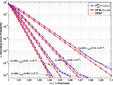
Figure IV.1: Curves in the figure represent EDEP (dashed in red) by (III.7), DEP (blue) by the S-MLDA, and KFRL (red) with destined error-bounds $\delta=10^{-4}$ for $n=200$, $10^{-5}$ for $n=300,400$, and $10^{-6}$ for $n=500$.

In this section, experimental results which show the viability of the EDEP for other block-lengths are presented. The truncated RSD in table III.1 was used for the experiments with the block lengths $n=200,300,400,500$.

By using EDEP’s with various fractions for $\rho_{n/2}$, we first investigated triple pairs of $(n,\rho_{n/2},\delta)$ for an optimal $\rho(x)$ in advance as shown in Fig. IV.1, where $\delta$ is a destined error-bound. With $(500,0.055,10^{-6})$, for example, the fraction $\rho_{250}=0.055$ is large enough for the supplementation $\rho(x)$, achieving the MSO $\gamma_{\min}(10^{-6},500,\rho)$ that is near the KFRO $\gamma_{K}(10^{-6},500)\approx 0.04$. Then with each optimized $\rho(x)$, we approximated the DEP by applying the S-MLDA over system (I.1). As can be seen clearly, each EDEP by $\rho(x)$ is almost identical to the DEP approximated by the S-MLDA, and also, it is very close to the limit $K(1+\gamma,n)$ up to a destined error-bound $\delta$.

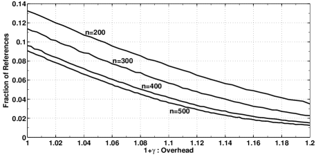
Figure IV.2: Curves represent the fractions $\epsilon=\frac{r}{n}$ with $n=200,300,400,500$ by the diagonal extension process over an $H$ by $\rho(x)$ used in Fig. IV.2

Let us now discuss the efficiency of LT decoding under the S-MLDA. To solve system (I.1), like other MLDA’s in [4, 5, 6], the S-MLDA uses an approximate lower-triangulation of $H$ in such a way that $\bar{H}=PHQ^{T}=\left[\begin{smallmatrix}A&B\\ C&D\end{smallmatrix}\right]$, where $(P,Q)$ is a pair of row and column permutations obtainable by the diagonal extension process in [4, 5, 15], and the right-top block $B$ is an $l\times l$ lower triangular matrix with $l=n-r$ close to $n$. The successful decoding by MPA in [7] is a particular case when $\left[\begin{smallmatrix}A\\ C\end{smallmatrix}\right]=\emptyset$. If $\left[\begin{smallmatrix}A\\ C\end{smallmatrix}\right]\neq\emptyset$ then the S-MLDA transforms $\bar{H}$ to $\left[\begin{smallmatrix}\bar{A}&I_{l\times l}\\ \bar{C}&0\end{smallmatrix}\right]$ by pivoting columns of the right-block $\left[\begin{smallmatrix}B\\ D\end{smallmatrix}\right]$ from the first to the last column of it, and then transforms the $r\times(r+\gamma n)$ block $\bar{C}$ to $\left[\begin{smallmatrix}I_{r\times r}\\ 0\end{smallmatrix}\right]$ by a conventional GE.

Let $r=\epsilon n$. Since $\bar{C}$ is not sparse in general, the decoding complexity of the transformation by the GE is $O((\gamma\epsilon^{2}+\epsilon^{3})n^{3})$. Hence the overall complexity of decoding by the MLDA’s is dominated by either $O((\gamma\epsilon^{2}+\epsilon^{3})n^{3})$ or the density $|H|$. Thus, although its overall complexity is $O(n^{3})$, the efficiency of the LT decoding under the S-MLDA can be measured in terms of the fraction $\epsilon=\frac{r}{n}$, and this is particularly true for short $n$.

In Fig. IV.2, curves represent the fraction $\epsilon=\frac{r}{n}$ obtained by the diagonal extension process on $H$ generated by the $\rho(x)$ used in Fig. IV.1. When $n=500$ and $1+\gamma=1.1$, for instance, the point $(1.1,0.038)$ indicates that, with a $550\times 500$ random $H$ by the $\rho(x)$ with $\rho_{n/2}=0.055$, the column-dimension of $\bar{C}$ is about $r=20$ that is much smaller than $n=500$ the column-dimension of $H$. This substantiates that decoding of the codes under the S-MLDA becomes very efficient as $\gamma$ increases.

V Summary

In Section II, a simple approach of generating a truncated RSD is presented. In Section III, explicit formulations of DEP and UBDEP are derived and utilized for obtaining an optimal $\rho(x)$, and KFRL is explained as a particular case of the conditional Kovalenko’s rank-distribution. In Section IV, experimental results which show the viability of the EDEP are presented.

References

- [1] M. Luby, LT Codes, Ann. IEEE Symp. on Foundations of Computer Science, 2002.
- [2] A. Shokrollahi, Raptor Codes, IEEE Trans. Inform. Theory, vol. 52, no.6, pp. 2551.2567, June 2006
- [3] David J.C Mackay, Information Theory, Inference and Learning Algorithms, Cambridge University Press 2003.
- [4] T. Richardson, R. Urbanke, Efficient Encoding of Low-Density Parity-Check Codes, IEEE Trans. Inform. Theory, 47:638-656, 2001.
- [5] David Burshtein, Gadi Miller, An Efficient Maximum-Likelihood Decoding of LDPC Codes Over the Binary Erasure Channel, IEEE Trans. Inform. Theory, 2004.
- [6] A. Shokrollahi, S. Lassen, and R. Karp, Systems and Processes for Decoding Chain Reaction Codes Through Inactivation U.S. Patent 1,856,263, Feb. 15, 2005.
- [7] M. Luby, M. Mitzenmacher, A. Shokrollahi, D. Spielman, Efficient Erasure Correcting Codes., IEEE Trans. Inform. Theory, 2001.
- [8] I. N. Kovalenko, A. A. Levitskaya and M. N. Savchuk, Selected Problems in Probabilistic Combinatorics (in Russian), Naukova Dumka, Kyiv 1986.
- [9] I. N. Kovalenko, On the Limit Distribution of the Number of Solutions of a Random System of Linear Equations in the Class of Boolean Functions (in Russian), Theory of Probab. Appl., 12:51-61, 1967.
- [10] C. Cooper, On the rank of random matrices, Random Structures and Algorithms, 1999.
- [11] V. F. Kolchin, Random Graphs, Cambridge University Press 1999.
- [12] Ki-Moon Lee and Hayder Radha, The Maximum Likelihood Decoding of LT codes and Degree Distribution Design with Dense Fractions, Proceedings on ISIT 2007.
- [13] Ki-Moon Lee, Hayder Radha, LT Codes from an Arranged Encoder Matrix and Degree Distribution Design with Dense Rows, Allerton Conference on Communication, Control and Computing 2007.
- [14] Ki-Moon Lee, Hayder Radha, and Beom-Jin Kim, Kovalenko’s Full-Rank Limit and Overhead as Lower Bounds of Error-Performances of LDPC and LT Codes over Binary Erasure Channels, ISITA 2008, Auckland, NZ, and submitted to Trans. Inform. Theory, June 2008
- [15] Ki-Moon Lee, Hayder Radha, and Beom-Jin Kim, Optimizing LT Codes with Dense Rows using Bounds in Decoding Error-Probability, submitted to Trans. on Comm. Theory, December 2008.