Best linear unbiased estimation of the nuclear masses

Abstract

This paper presents methods to provide an optimal evaluation of the nuclear masses. The techniques used for this purpose come from data assimilation that allows combining, in an optimal and consistent way, information coming from experiment and from numerical model. Using all the available information, it leads to improve not only masses evaluations, but also to decrease uncertainties. Each newly evaluated mass value is associated with some accuracy that is sensibly reduced with respect to the values given in tables, especially in the case of the less well-known masses. In this paper, we first introduce a useful tool of data assimilation, the Best Linear Unbiased Estimation (BLUE). This BLUE method is applied to nuclear mass tables and some results of improvement are shown.

keyword:

Data assimilation, Best Linear Unbiased Estimation, BLUE, nuclear masses, mass tables

1 Introduction

The mass tables provide an evaluation of the mass for every known and forecast nuclei and are very important in nuclear physic. Information gathered inside those table by experimentalist and various nuclear mass models (for example ”Finite-Range Liquid-Drop Model” [1, 2] or ”Finite-Range Droplet Model” [3]) is used for reaction planning and nuclear reactions simulations. Thus, an accurate knowledge of masses of the nuclei permits to realize high quality calculations and planning.

The purpose of this paper is to present a method to optimally evaluate masses of known nuclei, as well as the accuracy associated. The aim is to produce an improved set of data for nuclear masses, with better accuracy respect to tabulated ones. This general approach is already applied in other fields of science, as for example in meteorology, or oceanography or neutronic [4, 5]. The procedure proposed here is the same as the one climatologists use to obtain high accuracy meteorological data. This is the case for example of the widely used meteorological re-analysis ERA-40 [6]among others [7, 8].

Improving the accuracy of the data can be done in many ways, like in cumulating information from various experiments in a cleaver way to reduce the global inaccuracy, as presented in [9, 10, 11]. Such methods permit to converge toward a good accuracy of data. In the present case, we are interested in including information coming from a numerical model to the estimation of the value, and to the calculation of the associated accuracy. This approach is reasonable as the model is giving an overall information on the data, which means some constrains on the expected values for measurement. Data assimilation is precisely a general method to handle jointly experimental data and numerical modelling information to estimate the optimal values. Moreover, data assimilation techniques allow at the same time to improve accuracy of the estimation with respect to the original data.

In this paper, we will first develop some aspects on the theory and the basics concepts of data assimilation. In fact data assimilation covers a large number of techniques. Here we will focus on the Best Linear Unbiased Estimation (BLUE) technique, that fits very well to the present problem. We will use this BLUE technique to estimate the nuclear masses of the known nuclei found in the classical mass tables. This will lead to a new set of nuclear masses with improved accuracy.

2 Data assimilation

We briefly introduce the theory of data assimilation. However, data assimilation is a wide domain and we will not present here the advanced techniques that include dynamics of the process, that are for example the basis of the nowadays-meteorological operational forecast. Some interesting information on these approaches can be found in the following references [12, 13, 14]. More recently some applications of data assimilation have been done on nuclear core neutronic activity evaluation [15, 4, 5]

The ultimate goal of data assimilation methods is to be able to figure out the inaccessible true value of the system state, so called $\mathbf{x}^{t}$ with the $t$ index for ”true”. The basic idea of data assimilation is to put together information coming from an a priori on the state of the system (usually called $\mathbf{x}^{b}$, with $b$ for ”background”), and information coming from measurements (referenced as $\mathbf{y}$). The result of data assimilation is called the analysis $\mathbf{x}^{a}$, and it is an estimation of the true state $\mathbf{x}^{t}$ we want to find.

Some tools are necessary to achieve such a goal. As the mathematical space of the background and the one of observations are not necessary the same, a bridge between them needs to be built. This is the so called observation operator $H$, with its linearisation $\bf{H}$, that transforms values from the space of the background to the space of observations. The reciprocal operator is the adjoint of $H$, which in the linear case is the transpose $\bf{H}^{T}$ of $\bf{H}$.

Two other ingredients are necessary. The first one is the covariance matrix $\bf{R}$ of observation errors, which are $\epsilon_{o}=\mathbf{y}-H(\mathbf{x}^{t})$. It can be obtained from the known errors on the unbiased measurements. The second one is the covariance matrix $\bf{B}$ of background errors, which are $\epsilon_{b}=\mathbf{x}^{b}-\mathbf{x}^{t}$. It represents the error on the a priori, assuming it to be unbiased. There are many ways to obtain these observation and background error covariance matrices, such as kriging, stochastic simulation algorithms, ensemble estimation, etc (see for example [16, 17, 18]). However, this is commonly the output of a model and an evaluation of its accuracy, or the result of expert knowledge.

To find this optimal value $\mathbf{x}^{a}$ the underlying idea is to minimise the variance of the error $\epsilon_{a}=\mathbf{x}^{a}-\mathbf{x}^{t}$ associated to this value. Then it can be proved [14] that, within this formalism, the Best Unbiased Linear Estimator $\mathbf{x}^{a}$ is given by the following equation:

$$\mathbf{x}^{a}=\mathbf{x}^{b}+{\bf K}\big{(}\mathbf{y}-\mathbf{H}\mathbf{x}^{b}\big{)}$$ (1)

where ${\bf K}$ is the gain matrix:

$${\bf K}={\bf BH}^{T}({\bf HBH}^{T}+\mathbf{R})^{-1}$$ (2)

Moreover we can obtain the analysis error covariance matrix $\bf{A}$, characterising the analysis errors $\epsilon_{a}$. This matrix can be expressed from $\bf{K}$ as:

$$\mathbf{A}=(\mathbf{I-KH})\mathbf{B}$$ (3)

with $\mathbf{I}$ the identity matrix. Note that one way to prove equation 2 is to minimize the trace of the matrix $\bf{A}$, leading also to prove $\mathbf{x}^{a}$ is the optimal value we are looking for. The demonstration is detailed in the reference [14]. It can equivalently be proven through a maximum likelihood hypothesis. This lead on overall to an improvement of the accuracy, as it can be show in [9, 10, 11].

Then the main work is to evaluate as well as possible the observation operator ${\bf H}$ and the two covariance matrices $\mathbf{B}$ and $\mathbf{R}$. We will proceed with this task within the framework of the mass tables.

3 Application of data assimilation to the nuclear mass evaluation

To build the Best Linear Unbiased Estimation of the mass tables, we will work on masses excess instead of masses themselves. The mass excess of a nucleus is the difference between its actual mass and its mass number ($A\times u$) with $u$ the atomic mass unit, or ”unified atomic mass” (see Table A in [19] for information on this unit) and $A$ the number of nucleons.

For the background $\mathbf{x}^{b}$, we will take the reference data of mass excess values proposed in [20, 21] by P. Moller, J.R. Nix, W.D. Myers, and W.J. Swiatecki, focusing on the masses obtained from the Finite-Range Droplet Model [3] with shell energy correction. Note the results are very similar to the ones obtained from the Finite-Range Liquid-Drop Model [1, 2]. In those theoretical tables, we will limit ourselves to the known nuclei heavier than oxygen, that is with protons number $Z\geq 8$, which is the lowest reliable value for the model.

The experimental mass excess values are the one from G. Audi and all reference tables [22, 19, 23, 24]. This remarquable collection of data also includes the error associated to each measurement. This represents the observation, denoted $\mathbf{y}$ in the previous section.

These two data series of mass excess values $\mathbf{x}^{b}$ and $\mathbf{y}$ are in the same space. Then the required observation operator ${\bf H}$ is obviously reduced to identity ${\bf I}$.

The covariance matrix $\mathbf{R}$ on observation errors is chosen to be a diagonal matrix. On the diagonal, we put the known value of the uncertainties given in experimental tables [22, 19, 23, 24].

The evaluation of the background errors covariance matrix $\mathbf{B}$ is slighly more complicated. The first assumption is that background errors are independent the one from the other. Then $\mathbf{B}$ reduces to a diagonal matrix. As no information yet exists on the model accuracy, it is also assumed as a second assumption that this accuracy is independent of each nuclei we consider. Thus we only need one global value of accuracy denoted as $\sigma_{b}^{2}$. It remains to evaluate this unique value $\sigma_{b}^{2}$ on the diagonal. For this purpose, we made a statistical study. The error between $\mathbf{x}^{b}$ and $\mathbf{x}^{t}$ is overestimated by the error between $\mathbf{x}^{b}$ and ${\bf H}\mathbf{x}^{t}=\mathbf{y}$, that is globally more variable. Thus, considering that, last relative error gives a penalty to the accuracy on model evaluation. This is the third assumption we make to obtain model error evaluation. To evaluate a value for the diagonal of ${\bf B}$, we calculate the mean square of $\mathbf{x}^{b}-\mathbf{y}$ over all the available nuclei. The mean square is $\sigma_{b}^{2}=0.652904$, that is $\sigma_{b}=0.808024~{}MeV$. This is the value that we will put on the diagonal of $\mathbf{B}$.

For informative purpose, it is interesting to look at the calculated mean value of $\mathbf{x}^{b}-\mathbf{y}$, which it is equal to $-0.058326~{}MeV$. It is fairly close to $0$, and then comfort the implicit hypothesis to be in a quasi-unbiased case for background error estimation. It can be checked that the correlation between the background error and the measurement error is $0.1998$. This low value means that there are no significant correlation between those two error. Such a condition is required to use data assimilation under good condition.

All the required data are then available to build the data assimilation analysis as described in section 2, by simply applying formula 1. The differences between the experimental results $\mathbf{y}$ and the analysed results $\mathbf{x}^{a}$ obtained with data assimilation are shown on Figure 1 in percentage of change of mass excess for all the nuclei in function of their protons and neutrons numbers.

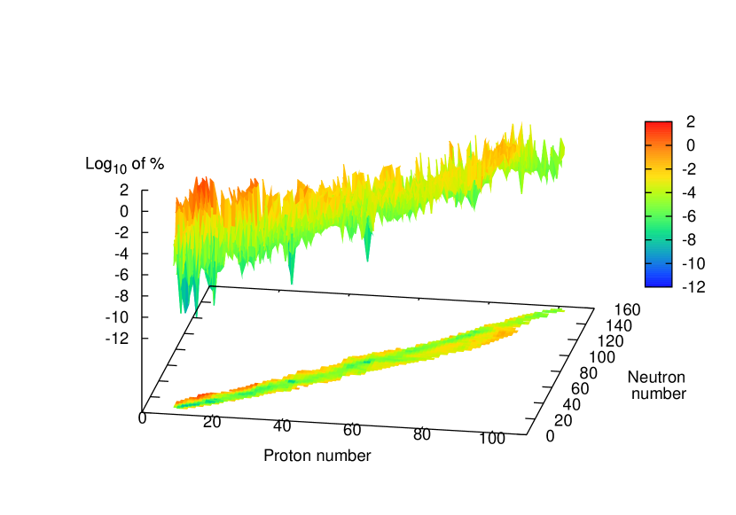
Figure 1: Mass excess experimental values percentage of change, as a function of the neutron and proton numbers of the nuclei.

On Figure 1, it can be noticed that the relative modification of the masses could be as lower as $10^{-10}\%$ up to $80\%$ in absolute value. This wide range of modification can be explained easily within an assimilation process. On the one hand, in case nuclei which masses are known very accurately, like for stable of nuclei, then information provided by the background (model) do not contribute a lot, masses excess do not change, and the relative modification is around $10^{-10}\%$. On the other hand, if nuclei masses excess are not known very accurately masses excess given by the model give a lot more information. Thus, information on physical property of nuclei included in the model allows to drive the measured value toward a new value that is more likely (in the sense of the maximum likelihood principle include in data assimilation method) and then modification can be up to $80\%$. Thus, as we notice on Figure 1, the more we go far from stability valley the more modification of the nuclei masses excess could be important because the less the experimental value are accurate due to the extreme difficulty to realize such measurement.

Considering those notable modification it is worth taking into account the new results for mass excess. We have checked that all results are correctly enclosed between the background previsions and the experimental values. This mean that we never overshoot either experimental value or the one given by the model. This result is in agreement with the modelling of ${\bf B}$ and ${\bf R}$ that have been done.

A key point is on the accuracy, as, by construction of the method, data assimilation improves it. The diagonal of the matrix ${\bf A}$ (which, in the present case, is a diagonal matrix) contains the variance $\sigma_{a}^{2}$ of the analysis $\mathbf{x}^{a}$ for each nuclear nuclei. We are looking at the percentage of evolution of the accuracy, with respect to the experimental accuracy $\sigma_{y}$ for each nuclei. Thus we can construct the following accuracy indicator $\frac{\sigma_{y}-\sigma_{a}}{\sigma_{y}}$, observed in percent.

With such a definition, an improvement of the accuracy (that is a decrease of $\sigma_{a}$ with respect to $\sigma_{y}$) is a positive percentage.

We have done two representations of those values. The first one is an histogram plot, where each bin represent the accuracy indicator for one nuclei, in order to get a 1D representation of all the results. To obtain such mono-dimensional plot, we consider the nuclei ordered in the same way as in the reference file [24]. Thus, the first bin correspond to the first nuclei of the G. Audi et al. table, and so on. The results are presented on the Figure 2. This representation allows to have a global overview of the amplitude of the modifications and of their values.

A second representation, two-dimensional, shows the results of the same relative accuracy as a function of the number of neutrons and protons. The results are presented on the Figure 3 (for representation reason, the scale of this figure is saturating at 10%). On this one, the crosses represent the nuclei that is the most accurately measured experimentally for each element. This gives a line close to the stability valley.

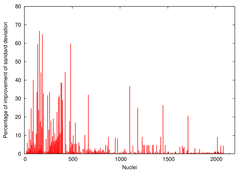
Figure 2: Percentage of improvement of the experimental error by the analysed error as a function of the number of the nuclei within the stables elements of table [24].

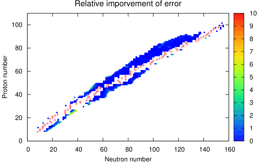
Figure 3: Percentage of improvement of the experimental error respect to the analysed error, as a function of the number of protons and neutrons. Each cross represents the nuclei that is experimentally the most accurately measured for each elements.

From Figure 2, we confirm that all values are positive, which means that there is always an improvement of the accuracy. The improvement can be up to roughly $70\%$ in some cases. As for the analysed value themselves, this means that when an experimental value is known very accurately, a lot of efforts are required to do better. On the contrary, if original accuracy on data is not so good, it is easy to improve it, providing only little additional information.

Considering Figure 3, from an experimental point of view, we notice that data assimilation provide value with an improved accuracy for the elements that are rather far from the stability line which usually mean the unstable nuclei. Those nuclei are often measured with lower accuracy that the sable one due to the intrinsic experimental difficulties.

Then, globally speaking, we can say data assimilation method applied to nuclear mass tables is very successful, and leads within a simple framework to some significant improvements of nuclei masses excess and their associated error.

4 Conclusion

Data assimilation technique applied on the mass tables seems then to be very promising. Here is described the generation of an optimal set of masses that can be used when needing mass tables information, as it was done in climatology by ERA-40 re-analysis [6]. The new mass data set produced will prove to be useful because:

• it shows to be within the limit previously given by theory and experience,

• the accuracies on the mass excess are lower than the one previously known, which makes them more suitable to use.

However, as a perspective, the present application is showing only some limited aspects of the possibility of data assimilation. Especially, the improvement of the $\mathbf{B}$ matrix can be studied in order to open the way for forecasting more accurately masses of yet unknown nuclei.

References

- [1] C.F. von Weizsacker. Zur theorie der kernmassen. Zeitschrift fur Physik, 96(7-8):431–458, 1935.
- [2] H.A. Bethe and R.F. Bacher. Stationary states of nuclei. Reviews of Modern Physics, 8:82–229, 1936.
- [3] P. Moller, W. D. Myers, W. J. Swiatecki, and J. Treiner. Nuclear ground-state masses and deformations. Atomic Data and Nuclear Data Tables, 39:225, 1988.
- [4] Bertrand Bouriquet, Jean-Philippe Argaud, Patrick Erhard, Sébastien Massart, Angélique Ponçot, Sophie Ricci, and Olivier Thual. Differential influence of instruments in nuclear core activity evaluation by data assimilation. Nuclear Instruments and Methods in Physics Research Section A, 626-627:97–104, 2011.
- [5] Bertrand Bouriquet, Jean-Philippe Argaud, Patrick Erhard, Sébastien Massart, Angélique Ponçot, Sophie Ricci, and Olivier Thual. Robustness of nuclear core activity reconstruction by data assimilation. Nuclear Instruments and Methods in Physics Research Section A, 629(1):282–287, 2011.
- [6] S.M. Uppala and al. Quaterly Journal of the Royal Meteorological Society, 131:2961–3012, 2005.
- [7] E. Kalnay and et al. The NCEP/NCAR 40-year reanalysis project. Bulletin of American Meteorological Society, 77:437–471, 1996.
- [8] G. J. Huffman and et al. The global precipitation climatology project (GPCP) combined precipitation dataset. Bulltin of American Meteorological Society, 78:5–20, 1997.
- [9] M.U. Rajput and T.D. MacMahon. Techniques for evaluating discrepant data. Nuclear Instruments and Methods in Physics Research Section A, 312(1-2):289–295, 1992.
- [10] S.I. Kafala, T.D. MacMahon, and P.W. Gray. Testing of data evaluation methods. Nuclear Instruments and Methods in Physics Research Section A, 339(1-2):151–157, 1994.
- [11] Desmond MacMahon, Andy Pearce, and Peter Harris. Convergence of techniques for the evaluation of discrepant data. Applied Radiation and Isotopes, 60(2-4):275–281, 2004.
- [12] O. Talagrand. Assimilation of observations, an introduction. Journal of the Meteorological Society of Japan, 75 (1B):191–209, 1997.
- [13] E. Kalnay. Atmospheric Modeling, Data Assimilation and Predictability. Cambridge University Press, 2003.
- [14] F. Bouttier and P. Courtier. Data assimilation concepts and methods. ECMWF, Meteorological Training Course http://www.ecmwf.int/, 1999.
- [15] Sébastien Massart, Samuel Buis, Patrick Erhard, and Guillaume Gacon. Use of 3DVAR and Kalman filter approaches for neutronic state and parameter estimation in nuclear reactors. Nuclear Science and Engineering, 155(3):409–424, 2007.
- [16] Jean-Paul Chilès and Pierre Delfiner. Geostatistics: Modeling Spatial Uncertainty. Wiley, 1999.
- [17] P. Goovaerts. Geostatistical modelling of uncertainty in soil science. Geoderma, 103(1-2):3–26, 2001.
- [18] Haiyan Cheng, Mohamed Jardak, Mihai Alexe, and Adrian Sandu. A hybrid approach to estimating error covariances in variational data assimilation. Tellus, 62(3):288–297, 2010.
- [19] A. H. Wapstra, G. Audi, and C. Thibault. The ame2003 atomic mass evaluation: (i) evaluation of input data, adjustment procedures. Nuclear Physics A, 729 (1):129–336, 2003.
- [20] P. Moller, J.R. Nix, W.D. Myers, and W.J. Swiatecki. Nuclear ground-state masses and deformations. Atomic Data and Nuclear Data Tables, 59 (2):185–381, 1995.
- [21] P. Moller, J.R. Nix, W.D. Myers, and W.J. Swiatecki. http://ie.lbl.gov/, Atomic Data and Nuclear Data Tables file ’astab.txt’, 1995.
- [22] G. Audi, O. Bersillon, J. Blachot, and A.H. Wapstra. The nubase evaluation of nuclear and decay properties. Nuclear Physics A, 729 (1):3–128, 2003.
- [23] G. Audi, A.H. Wapstra, and C. Thibault. The ame2003 atomic mass evaluation: (ii) tables, graphs and references. Nuclear Physics A, 729 (1):337–676, 2003.
- [24] G. Audi, A.H. Wapstra, and C. Thibault. Atomic Mass Data Center (AMDC), http://amdc.in2p3.fr/, Atomic mass adjustment file ’mass.mas03’, 2003.