Candidate microlensing events from M31 observations with the Loiano telescope

Abstract

Microlensing observations towards M31 are a powerful tool for the study of the dark matter population in the form of MACHOs both in the Galaxy and the M31 halos, a still unresolved issue, as well as for the analysis of the characteristics of the M31 luminous populations. In this work we present the second year results of our pixel lensing campaign carried out towards M31 using the $152~{}\mathrm{cm}$ Cassini telescope in Loiano. We have established an automatic pipeline for the detection and the characterisation of microlensing variations. We have carried out a complete simulation of the experiment and evaluated the expected signal, including an analysis of the efficiency of our pipeline. As a result, we select 1-2 candidate microlensing events (according to different selection criteria). This output is in agreement with the expected rate of M31 self-lensing events. However, the statistics are still too low to draw definitive conclusions on MACHO lensing.

1. Introduction

The search for microlensing events aimed at the characterisation of the MACHO distribution in galactic halos, first discussed by Paczyński (1986), is by now an established technique. The results obtained up to now are, however, debated. Towards the LMC the MACHO group have claimed the detection of a MACHO signal from objects of $\sim 0.4~{}\mathrm{M}_{\odot}$ that would constitute a halo mass fraction of about $f\sim 0.2$ (Alcock et al., 2000; Bennett, 2005), whereas the EROS group have found no candidate microlensing events and put a rather stringent upper limit on the same quantity, $f<0.1$ in the MACHO mass range preferred by the MACHO results (Tisserand et al., 2007). The issue of the nature of the detected candidates still remains an open question (Sahu, 1994; Wu, 1994; Mancini et al., 2004; Calchi Novati et al., 2006; Evans & Belokurov, 2006).

The contradictory results obtained towards the Magellanic Clouds challenge one to probe the MACHO distribution along different lines of sight. Beyond the Galaxy, M31 represents the next most suitable target for microlensing searches (Crotts, 1992; Baillon et al., 1993; Jetzer, 1994). Looking at it from outside, we can globally study the M31 halo; the line of sight towards M31 allows one to probe the Galactic halo along a different direction; the inclination of the M31 disk is expected to give a clear signature in the spatial distribution for microlensing events due to lenses in the M31 halo. Several observational campaigns have been carried out: AGAPE (Ansari et al., 1997), who presented the first convincing microlensing candidate along this line of sight (Ansari et al., 1999), Columbia-VATT (Crotts & Tomaney, 1996), POINT-AGAPE (Aurière et al., 2001; Paulin-Henriksson et al., 2003), SLOTT-AGAPE (Calchi Novati et al., 2002, 2003), WeCAPP (Riffeser et al., 2003), MEGA (de Jong et al., 2004), NainiTal (Joshi et al., 2005). The detection of a few microlensing candidates has been reported, as well as first, though contradictory, conclusions on the MACHO content along this line of sight. The POINT-AGAPE group have reported evidence of a MACHO signal (Calchi Novati et al., 2005), whereas the MEGA group have concluded that their detected signal is compatible with the expected M31 self-lensing rate (de Jong et al., 2006). Very recently, Riffeser et al. (2008) have presented a new analysis of a previoulsy reported bright event observed towards the M31 central region. Taking into account the effects of the source’s finite size, they have concluded that the lens of this event should be attributed to the MACHO population. Finally, we recall that a few interesting attempts have also been proposed (Totani, 2003), or already carried out (Baltz et al., 2004), towards targets located beyond the Local Group.

In 2006 we began a new observational microlensing campaign towards M31 using the Cassini $152~{}\mathrm{cm}$ telescope at the “Osservatorio Astronomico di Bologna” (OAB) located in Loiano. The results of the first year pilot season have been discussed in Calchi Novati et al. (2007). In this paper we discuss the second year campaign. As the main result, we have carried out a complete analysis of the microlensing flux variations, selected two microlensing candidates and compared them with the expected microlensing signal. In Sect. 2 we present the observational setup and outline our data reduction and analysis technique. In Sect. 3 we present our pipeline for the search for microlensing-like flux variations. In Sect. 4 we present the simulation of the experiment with an evaluation of the expected signal. In Sect. 5 we discuss the main results of the present analysis. Finally, in the Appendix we describe in some detail some of the steps of our selection pipeline and of our Monte Carlo scheme.

2. Data analysis

2.1. Observational setup, data acquisition and reduction

The data have been collected at the $152~{}\mathrm{cm}$ Cassini Telescope located in Loiano (Bologna, Italy). We make use of a CCD EEV of $1340\times 1300$ pixels of $0.58^{\prime\prime}$ for a total field of view of $13^{\prime}~{}\times~{}12.6^{\prime}$, with gain of $1.0\mathrm{e}^{-}$/ADU (this value has changed with respect to that of the first season because of some electronics problems) and low read-out noise (3.5 e^-/px). We have been monitoring two fields of view around the inner M31 region, centered respectively in RA=$0{\mathrm{h}}42{\mathrm{m}}50{\mathrm{s}}$, DEC=$41^{\circ}23^{\prime}57^{\prime\prime}$ (“North”) and RA=$0{\mathrm{h}}42{\mathrm{m}}50{\mathrm{s}}$, DEC=$41^{\circ}08^{\prime}23^{\prime\prime}$ (“South”) (J2000), so to leave out the innermost ($\sim 3^{\prime}$) M31 bulge region, and with the CCD axes parallel to the south-north and east-west directions so to get the maximum field overlap with previous campaigns. This second year campaign lasted 50 consecutive full nights, from November 11 to December 31, 2007, with a fraction of good weather of almost 60%. In order to test for achromaticity, data have been acquired in two bandpasses (similar to Cousins $R$ and $I$), with exposure times up to 6 minutes per frame. Overall we collected about 410 (280) exposures per field over 31 nights in the $R$ ($I$) band. Typical seeing values are $\sim 2^{\prime\prime}$ (somewhat worse than during the first season). Sky flat frames were taken whenever possible so as to build a master flat image (per filter), and standard data reduction, including bias subtraction, was carried out using the IRAF package. We corrected $I$ filter data for fringe effects. The analysis presented in this paper is based on the 2007 season data only.

2.2. Image analysis

As for the preliminary image analysis we closely follow the strategy (the “pixel-photometry”) adopted by the AGAPE group (Ansari et al., 1997; Calchi Novati et al., 2002), wherein each image is geometrically and photometrically aligned relative to a reference image. To account for seeing variations we then substitute the flux of each pixel with that of the corresponding 5-pixel square “superpixel” centered on it (whose size is chosen so to cover most of the average seeing disk) and then apply an empirical, linear, correction in the flux, again calibrating each image with respect to the reference image. The final expression for the flux error accounts both for the statistical error in the flux count and for the residual error linked to the seeing correction procedure. Finally, in order to increase the signal-to-noise ratio, we combine the images so to get 1 data point per night per filter.

We evaluate the calibration zero point for the instrumental magnitude versus standard $(RI)_{C}$ magnitudes by using a sample of secondary reference stars (Massey et al., 2006). We find for $R$ and $I$ bands data $C_{R}=23.1$ and $C_{I}=22.7$, respectively (the reported values corresponding to the standard magnitude for an object with instrumental magnitude of $1~{}\mathrm{ADU~{}s}^{-1}$).

3. Microlensing event search pipeline

We have established a fully automated pipeline for the detection and the characterisation of microlensing-like flux variations. We work in the “pixel-lensing” regime (Gould, 1996), in which one looks for flux variations whose sources are not resolved objects, so that one has to monitor flux variations of every element of the image, further characterized by the fact that the noise is dominated by the underlying background level (the varying M31 surface brightness). As for this specific analysis, our strategy starts from that described in Calchi Novati et al. (2005) with a few changes introduced to take into account the peculiarities of the present data set.

During the analysis we have to face two main sources of contamination: “fake” signals, namely spurious variations to be attributed to cosmic rays, defects in the CCD, saturated pixels and so on; background intrinsically variable objects, that can either mimic microlensing signals or, somewhat more dangerously, add non-Gaussian noise to the light curves.

Our pipeline can be schematically divided into four steps. First: detection of the potentially interesting flux variations. Second: characterisation of the light curve shape. Third: probe against the contamination by spurious detections. Fourth: probe against the contamination by variable signals.

3.1. Bump detection

As for the first step we closely follow the strategy outlined in Calchi Novati et al. (2003, 2005). To begin, we detect flux variations along light curves using the $L$ estimator (we ask $L>50$ to get rid of too small S/N variations). Each given flux variation enhances a signal over a few pixels (a “cluster”) around the central one. We make use of the “$Q$” estimator to characterize the significance of the selected flux variations. We fix a lower threshold $Q_{\mathrm{th}}=50$. At this stage, therefore, we have to shift from the light curve analysis (the estimation of $L$ and $Q$), to an analysis based on the spatial information across the CCD in which we have to distinguish, separate and pick up the flux variations associated to each different cluster. This search is somewhat biased in favour of light curves showing a single variation (in particular, all short period variables are in principle excluded). This first step is carried out using the (more numerous and less noisy) $R$ band data only.

3.2. Light curve shape

The aim of the second step is to single out the variations whose shape is compatible with that of a Paczyński light curve. To this end, we use a series of selection criteria. As a starting point we perform a 7-parameter Paczyński fit in the two bands simultaneously. As an output we retain the following parameters: the baseline levels; the time of maximum magnification, $t_{0}$; the full-width-at-half-maximum duration, $t_{1/2}$ (proportional to the Einstein time, $t_{\mathrm{E}}$, multiplied by a function of the impact parameter $u_{0}$); the flux deviation at maximum (with respect to the baseline), which we convert to magnitude and denote $\Delta R$, together with the color of the variation, $R-I$, ($\Delta R$ is proportional to the source flux, $\phi^{*}$, multiplied by a function of the impact parameter); and the reduced $\chi^{2}$ of the fit. We make use of the full parametrisation of the Paczyński fit, looking for the Einstein time, the magnification and the unlensed source flux values, even if the intrinsic parameter degeneracy (linked to the fact that the source is not resolved), in most cases, does not allow one to accurately estimate the single parameters. As a selection criterion we ask $\chi^{2}/\mathrm{dof}<10$. This rather high threshold is motivated by the necessity to handle light curves contaminated by low level noise of non-Gaussian nature that can be attributed in particular to nearby blended intrinsic variables.

As a second test on the shape, we ask for the bump to be suitably sampled by the observed data points. We split our analysis on the basis of a more or a less demanding requirement, so that we are going to refer to set “A” and set “B” of candidates, respectively. The details are given in the Appendix A.

As a final test on the shape, we look at the characteristics of the detected flux variations. The two relevant parameters are the event duration, $t_{1/2}$, and the flux deviation at maximum, $\Delta R$. In order to appropriately delimit these parameter spaces, we have to balance for the efficiency, the expected event characteristics and the risk of contamination of the background of variable stars. We introduce a cut to exclude too faint variations, too noisy and therefore difficult to distinguish against the variable contamination. As a selection criterion, we ask for $\Delta R<21.5$. As for the duration, we do not expect microlensing events to last more than 10-20 days (Sect. 4.1). Besides, we expect long-duration variations to be heavily contaminated by intrinsic variable signals. However, we prefer not to introduce any cut for this parameter allowing for long duration candidates. As detailed below, all of these are rejected in the following steps of the analysis anyway.

3.3. PSF shape: spurious detection

Up to now the analysis is based on the light curve pixel-photometry only (besides the initial “cluster” analysis), in particular we do not make use of the PSF of the flux variations we are looking for. In this respect our approach is completely different from that based on the difference image analysis. As it is, however, this approach suffers from a high risk of contamination by spurious variations. To reject them in an automated way, as a third step we perform an extremely rough difference image analysis. The underlying rationale is that, whenever we detect a variation on a light curve, in order to retain it we want to “see” a corresponding well shaped PSF when we look at the image difference of the maximum magnification minus the baseline. Futher details are given in the Appendix B.

3.4. Variable signals

As a fourth and final step we probe the surviving variations against the background of variable contamination. Our limited baseline, 50 days, does not allow us by itself to carry out this programme. For this reason we make use of the 3-years baseline of the POINT-AGAPE data set. The rationale is that we want to reject flux variations that show variability along the much longer INT baseline with a comparable flux deviation to that detected on our OAB data. As a first step, given the OAB detected variation, we look for the corresponding pixel within the POINT-AGAPE data set. To probe variability along the INT light curve we use a Lomb periodogram analysis. As an estimator, we use the power “$P_{R}$” as defined in Numerical Recipes (Press et al., 1992). Second, we test whether the INT and the OAB flux deviations are compatible. To this end, given a relative flux calibration between the two data sets, first we rescale the OAB flux deviation; then we evaluate the difference of the observed flux deviations (the rescaled OAB minus the INT one), normalized by the INT error. We take this quantity, which we define $\delta(\Delta f)$, as our estimator. As a selection criterion, we ask for $P_{R}<20$ or $\delta(\Delta f)>5$.

4. The expected microlensing signal

In order to gain insight into the observed signal, first of all we have to evaluate the expected signal for our experimental set up. We briefly outline our approach as follows (Calchi Novati et al., 2005). First, we run a Monte Carlo simulation whose purpose is to give us the characteristics, and in particular the number, of the expected microlensing events. To this end, we have to specificy an astrophysical model and a model for the microlensing magnification, besides reproducing as closely as possible the actual experimental conditions. As for this last point, to account for those aspects of our pipeline that can not be accurately reproduced within the Monte Carlo, we carry out a simulation on the real data set of the events selected within the Monte Carlo.

4.1. The model

We consider the bulge and the disk populations of M31 as sources, both M31 bulge and disk stars as lenses (we refer to these events as “M31 self lensing”), and MACHOs in both the M31 and the Milky Way dark matter halos. We assume an M31 distance of $770~{}\mathrm{kpc}$.

As a model for the M31 luminous components we take the Kent (1989) bulge-disk decomposition, including the bulge ellipticity, and with the missing information of the vertical distribution of the disk modeled with a $\mathrm{sech}^{2}$ law and scale height of $300~{}\mathrm{pc}$. For both halos we assume a spherical isothermal distribution with a core radius $a=5~{}\mathrm{kpc}$.

The peculiarity of M31 microlensing is that we look for flux variations of unresolved sources. The issue of estimating the number of available sources is therefore particularly delicate. To this end, we consider the value of the M31 surface brightness (as given by Kent 1989) and the underlying luminosity function. As has already been remarked (Ansari et al., 1997), it turns out that only luminous sources (about $M_{I}<2$) are expected to give rise to detectable events. In the most crowded region, this may sum up to hundreds of available source stars per pixel (this can be considered as a completely blended situation with respect to, for instance, studies towards the LMC). As for the luminosity function that we use to characterize the sources, it is worth stressing that we are most interested in its bright end (even if we need the information over the complete magnitude range for the normalisation), whereas, for the mass function that we need for the luminous lenses, we are rather interested into the opposite tail.

We have made use of the IAC-star software (Aparicio & Gallart, 2004) to build a synthetic luminosity function for the M31 bulge, following the procedure outlined in Bozza et al. (2008), in particular as for the metallicity distribution (Sarajedini & Jablonka, 2005), with the difference that we have now used, as a mass function, a power law $\xi(m)\propto m^{-\alpha}$ with index $\alpha=1.33$ up to $1~{}\mathrm{M}_{\odot}$ and $\alpha=2$ above. For bulge lenses we have for consistency used the same mass function with upper bound fixed at one solar mass. For the disk luminosity function, as in Calchi Novati et al. (2005), we make use of the local neighborhood data obtained by Hipparcos corrected at the bright end (Perryman et al., 1997; Jahreiß & Wielen, 1997). For the disk lens mass function we follow as well the local determination (Kroupa, 2007) with upper bound fixed at $10~{}\mathrm{M}_{\odot}$. For MACHO masses we try a set of single values ranging from $10^{-3}$ to $1~{}\mathrm{M}_{\odot}$.

We fix the total mass of the bulge to $4\times 10^{10}~{}\mathrm{M}_{\odot}$ (Kent, 1989) (this can be considered a “safe” value for microlensing analyses, for the purpose of evaluating the expected self-lensing signal, as it is likely to be an upper limit (Riffeser et al., 2006) for this quantity), and that of the disk to $3\times 10^{10}~{}\mathrm{M}_{\odot}$ (Kerins et al., 2001; Riffeser et al., 2006). Looking for microlensing effects, the value we are actually interested in is the stellar mass, and indeed our overall value for this quantity agrees well with the analysis of Tamm et al. (2007). We consider a uniform extinction across the field, both foreground, $E(B-V)=0.062$ (Schlegel et al., 1998), and intrinsic (for this second term, this hypothesis should of course be taken only as a first order approximation), $\mathrm{ext}_{R}=0.19$ for the bulge (Han, 1996; Riffeser et al., 2006) and $E(B-V)=0.22$ for the disk (Stephens et al., 2003; Riffeser et al., 2006). Together with the M31 color (not corrected for extinction) $B-r=1.3$ (Kent, 1989), $B-V=1.0$ and $V-R=0.8$ (Walterbos & Kennicutt, 1987), this translates into the values (corrected for extinction) $M/L_{R}=3.1,\,1.1$, for the bulge and disk respectively.

The bulge velocity distribution is dominated by its dispersive component, with line of sight velocity dispersion of $\sigma=120~{}\mathrm{km~{}s}^{-1}$. For the disk we take into account both the dispersive motion, $\sigma=60~{}\mathrm{km~{}s}^{-1}$ (a value that can be taken as un upper limit), and a circular bulk motion, with disk circular velocity $v=250~{}\mathrm{km~{}s}^{-1}$ (Carignan et al., 2006). M31 proper motion is set according to van der Marel & Guhathakurta (2008).

Given the values of the circular velocity, $220~{}\mathrm{km~{}s}^{-1}$ and $250~{}\mathrm{km~{}s}^{-1}$ for the Milky Way and M31 respectively, we fix accordingly the central densities and therefore the overall masses of the halos and the values of the one dimensional velocity dispersions. As for the total dark matter halo mass value, within a truncation radius of $100~{}\mathrm{kpc}$ and $130~{}\mathrm{kpc}$ for the Milky Way and M31 (we estimate the ratio of these values from those of the circular velocities), we have respectively $1.0\times 10^{12}~{}\mathrm{M}_{\odot}$ (in good agreement with previous determination, e. g. Vallenari et al. (2006), but somewhat in excess with respect to the recent determination by Xue et al. 2008) and $1.8\times 10^{12}~{}\mathrm{M}_{\odot}$.

4.2. The simulation

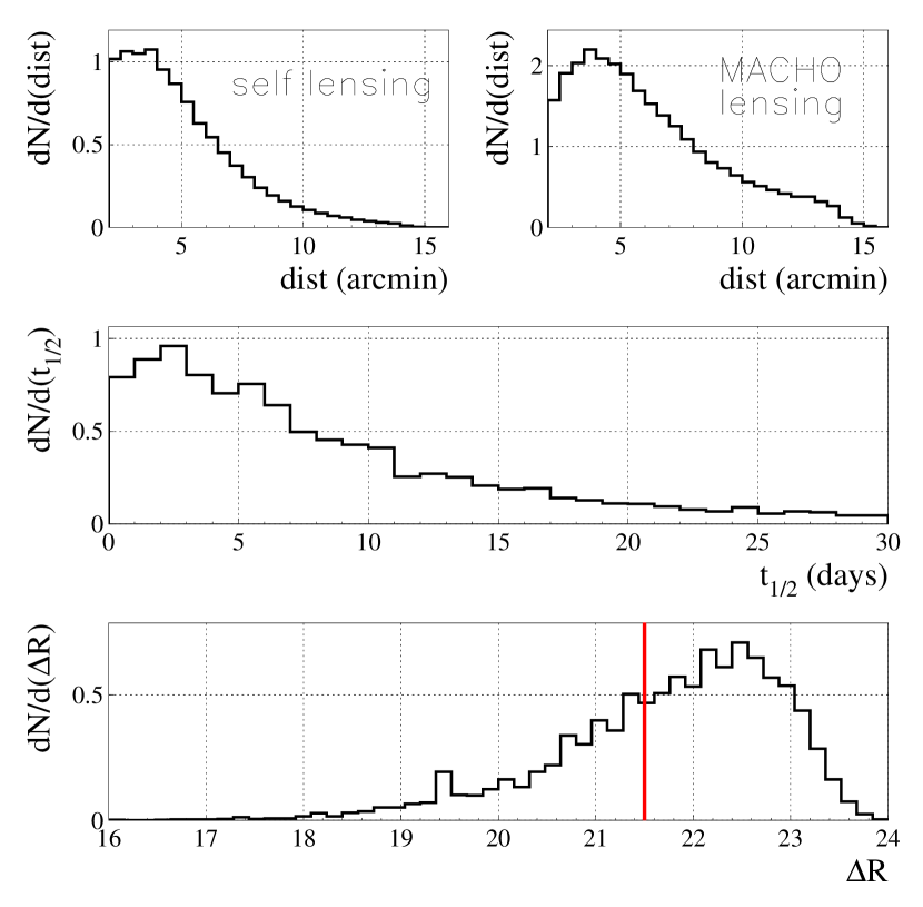
Figure 1.— Characteristics of the expected events from the Monte Carlo analysis. From top to bottom: histograms for the distance from the M31 center, duration (full-width-at-half-maximum) and the flux deviation at maximum magnification. Histograms for event duration and flux deviation are given for self lensing only. For all of the histograms we show all of the events selected, namely for the full range of the parameters. In the bottom panel, the solid line indicates the threshold value we use in the pipeline.

Within the Monte Carlo simulation, given the astrophysical model, we generate microlensing signals with Paczyński magnification corrected for finite size effects of the sources, build the correspoding light curves and carry out a first rough selection, paying attention not to reject any light curve that could be detected through our pipeline. In particular, for a variation to be selected, as a unique criterion we ask for at least 3 consecutive points (with one point per night and reproducing the observed sampling) 3 sigma above the backrgound level ($L>0$ according to the estimator introduced in Sect. 3). On the other hand, we are aware that we can not reproduce within the Monte Carlo, where we only deal with light curves, all of the the actual conditions of the pipeline we carry out in the real data set (where the analysis starts from the images). Amongst other effects, we most prominently can not reproduce crowding effects, the underlying variable signals and the sources of non-Gaussian noise. Furthermore, we can not run the first essential step of bump “cluster” detection. To account for these effects we simulate those light curves that are selected within the Monte Carlo on the images (before the geometrical and all photometric corrections, namely, on the astronomical images just after the basic bias-flat fielding reductions) and then we run from scratch our pipeline. Conceptually, this is just a last step in the Monte Carlo that allows us to accurately evaluate the efficiency of our pipeline. The “efficiency”, hereafter, should therefore be intended as that relative to the light curves selected within the Monte Carlo.

Within the Monte Carlo each simulated event carries a (different) “weight”, $w_{i}$ (where $i$ is the index of the simulated events) that is linked in part to the drawing process and in part to the quantity we are evaluating (the microlensing rate), and is completely independent of the selection process. The expected number of events is therefore the sum of the weights, $n_{\mathrm{exp}}=\sum_{i}w_{i}$, where the sum runs over the events selected within the Monte Carlo (correspondingly we can estimate the associated statistical error based on Poisson statistics). Accordingly, by “efficiency”, $\epsilon_{w}$, we mean the ratio of selected over simulated events, where the number we refer to is always given by the sum of the weights. This is usually different (both numerically and from a logical point of view) from the actual ratio of selected over simulated events, a quantity that is not used even if in some cases it may be useful to be looked at. In particular, we do not expect, and in fact we do not find, these two values to be too different. Indeed, such a result should be taken as a hint of the presence of some bias in the way the event weights are distributed with respect to the selection process within the simulation.

For each lens population, we simulate up to a few thousands events per field, with 500 events per field per simulation in order to avoid overlap problems. Indeed, in particular in the inner M31 region, where we expect most of the events, simulated events may overlap (we draw at random from the Monte Carlo the events we simulate, with all their characteristics, including the line of sight) and thus lead us to bias the estimate of the efficiency of our pipeline. To test for this effect, for a fixed set of 500 events per field for which we had already evaluated the efficiency, we have carried out as many different simulations as needed, taking care to leave a minimum distance of at least 20 pixels among any couple of generated events, so to exclude overlap problems. As a result, we have found no significant differences in the two analyses. Overall, we have simulated 12000 light curves to evaluate self-lensing efficiency, and 8000 for each value of the mass for MACHO lensing.

According to the selection pipeline, in which we require for the flux variations to be large enough, $\Delta R<21.5$, out of the Monte Carlo we extract, and then simulate on the images, selected events with flux deviation at maximum down to $\Delta R=21.8$. This limit is used accordingly when we evaluate the number of expected events. This way we allow for the observed rms of the evaluated flux deviations versus the input values. The exact value of this threshold is not, however, essential, as long as we keep the selection criterion on the flux deviation fixed at $\Delta R<21.5$ coherently with the selection pipeline. A brighter threshold would translate into a larger value for the efficiency and, at the same time, a smaller number of expected events (not corrected for the efficiency), and vice versa. These two effects balance when we evaluate the number of expected events corrected for the efficiency.

As for the expected characteristics of the observed events, in Fig. 1 we show the resulting distributions for the distance from the M31 center (both self lensing and MACHO lensing), and, for self lensing, the distribution for the durations (the full width at half maximum $t_{1/2}$) and the flux deviations at maximum ($\Delta R$).

Finally, it is worth stressing that we simulate microlensing events only. Therefore the simulation is restricted to saying whether and how our pipeline is going to select microlensing signals but it can say nothing about whether it might select as a microlensing a variable signal of different origin.

5. Results

In this Section we present and discuss the results of our analyses: the selection pipeline for microlensing flux variations and the evaluation of the expected microlensing signal.

5.1. The selection pipeline

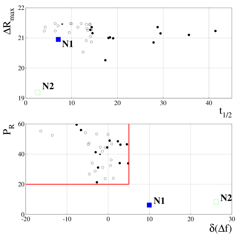
Figure 2.— Selection pipeline results: the sample shown here consists of the light curves selected after the PSF analysis. Scatter plot of the flux deviations versus the event duration (top panel); scatter plot of the Lomb “power” $P_{R}$ versus the relative flux difference $\delta(\Delta f)$ (filled and empty symbols for set A and B variations, respectively). The squares indicate the two candidate microlensing events of our selection (according to the terminology introduced in Sect. 5.2). The solid lines delimit the excluded region (bottom panel, upper left corner) in the last step of the analsyis. The star symbol indicates the second event, beside N1, belonging to both set A and set B. Bottom panel : for visualisation purposes we do not show a few rejected events with $\delta(\Delta f)<0$ and $P_{R}>20$.

Figure 3.— INT and OAB $R$-band light curves extension of 4 out of the 14 set A flux-variations OAB candidate microlensing events selected after the shape and the PSF analyses (left and right panels, respectively). The solid lines mark the evaluated baseline level, while the dotted lines show the maximum flux deviation value along the detected OAB flux variation (right panels) and this same value once rescaled on the INT data set (left panels). For each INT data light curve we indicate the result of the Lomb periodogram analysis, the power $P_{R}$, and the difference of the flux deviation along the OAB and the INT light curves, $\delta(\Delta f)$. The units on the $x$ axes are time in days (JD-2450000.0). The ordinate axes units are flux in ADU s^-1 per superpixel.

Table 1Microlensing selection pipeline : the results

	selection		simulation
criterion	# events		efficiency $\epsilon_{w}$ (%)
	set A	set B	set A	set B
bump detection	4200		$41.2\pm 3.5$
$L_{1}>50$	3033		$35.5\pm 3.2$
shape analysis
$\chi^{2}/\mathrm{dof}<10$	2901		$32.7\pm 3.0$
sampling	174	241	$18.3\pm 2.0$	$21.9\pm 2.4$
$\Delta R<21.5$	75	108	$13.0\pm 1.5$	$20.4\pm 2.3$
PSF	14	23	$13.0\pm 1.5$	$15.7\pm 1.9$
variable	1	2	$11.9\pm 1.4$	$14.6\pm 1.8$

Note. — The results of the selection pipeline for microlensing light curves: analysis and simulation. For each step we report the number of selected light curves and the efficiency of the pipeline (%) for the expected self-lensing signal. According to the choice of the sampling criterion, we have split our selection results in set A and set B (left and right column, respectively).

In Table 1 we report the results of the selection pipeline analysis together with the results for the efficiency of the corresponding analysis carried out on self-lensing simulated events.

We start the analysis working over the complete set of pixels, namely $2\times(1340\times 1300)$ light curves. The initial sample of selected flux variations consists of $\sim 4000$ light curves. Within the shape analysis, the sampling cut severely reduces this initial set, and then the flux deviation cut leaves us with $\sim 200$ light curves, most of which, according to the PSF analysis, are to be attributed to spurious variations. Finally we are left with $\sim 40$ flux variations, divided into sets A and B (according to the sampling criterion), most of which we expect to be intrinsic variables whose single-bump appearance is to be attributed to our short (50 days) baseline. (As outlined in Appendix A, set A flux variations are not a subsample of set B: among those surviving the PSF cut, 14 and 23 respectively, only two flux variations are in common between the two data sets, out of which one also survives the last cut.) The results of the last cut analysis are shown in the bottom panel of Fig. 2 in the parameter space $P_{R}$-$\delta(\Delta f)$. We find, as expected, the flux deviation of most OAB variations to be compatible with the corresponding INT variations (small values of $\delta(\Delta f)$), for which, at the same time, we find a clear sign of variability (large value of $P_{R}$). As an example, in Fig. 3, we show the INT extension of 4 OAB selected light curves. Only for two selected OAB flux variations, instead, we find the corresponding INT extension to be flat. Therefore the selection pipeline finally leave us with two microlensing candidates (one belonging to set B only). The same sample of light curves is represented in the $\Delta R_{\mathrm{max}}-t_{1/2}$ parameter space (top panel of Fig. 2). We find most of the variations located in the upper part (corresponding to small flux deviations), with set B variations (empty symbols) biased towards short durations. In particular we find the set A microlensing candidate (filled square symbol) located in a parameter space region where the contamination by the intrinsic variable signals is large. The only clear outlier is the bright and short set B microlensing candidate. We discuss the selected candidates in detail in Sect. 5.2.

Comparing with the efficiency simulation analysis, a few points are worth being mentioned. First, it may look as if the “bump detection” step alone severely reduces the overall efficiency. However, in fact, only a very small fraction of light curves that are not selected at this point would pass all the other criteria. According to the same principle, the single cut that excludes most of the simulated light curves is the sampling criterion. This is also the reason why we have split our selection pipeline at this level. As for the simulation, we stress that this simply reflects the choice we have made in the Monte Carlo to select light curves on the basis of the $L>0$ criterion only. Next, the PSF analysis proves to be a rather efficient criterion. Indeed it results that almost 50% of the simulated light curves fulfill this criterion and that this fraction rises to about 80% if we consider the subset of light curves that have already passed the bump detection and the shape analysis cuts. A usual reason that may cause the PSF Gaussian fit to fail is the presence, near the simulated event, of some other resolved object. Often enough, however, in these cases also the pixel photometry we use may have problems. (For both of these related aspects, a proper difference image analysis approach would be of course expected to give better results). Poorly sampled light curves, on the other hand, simply do not have enough points near maximum magnification, so that it turns out to be usually not possible to carry out a good enough PSF fit. Finally, as for the analysis on the POINT-AGAPE extension to check for variable signals, we have seen this cut to be essential to get rid of otherwise dangerous contaminating flux variations. At the same time, this shows to be an extremely efficient criterion. Out of the complete set of simulated light curves, only about 13% of the INT light curves are clearly variable ($P_{R}>20$) and this fraction falls to 7% when we add the demand for the INT flux deviation to be compatible with the OAB simulated one.

Table 2Efficiency analysis: the results for MACHO lenses.

mass ($\mathrm{M}_{\odot}$)	efficiency $\epsilon_{w}$ (%)
	set A	set B
1	$16.5\pm 1.2$	$18.7\pm 0.9$
0.5	$18.5\pm 1.1$	$21.3\pm 1.2$
0.1	$16.5\pm 1.2$	$19.9\pm 1.4$
$10^{-2}$	$13.8\pm 1.2$	$16.5\pm 1.3$
$10^{-3}$	$11.1\pm 1.3$	$13.2\pm 1.4$

In Table 2, we report the results for the efficiency of the simulations for MACHO lenses. With respect to self-lensing events there is a (rather small) effect linked to the different spatial distribution. The main effect is, however, due to the value of the mass, which is linked to the event duration, with smaller values of the efficiency corresponding to decreasing values of the MACHO lens mass.

In Tables 1 and 2 we have given the results for the efficiency as a single value for the overall set of simulated events. On the other hand, the efficiency does vary quite significantly for data binned, for instance, in the distance from the M31 center and/or in the flux deviation at maximum. We find the larger values for the efficiency, up to 30% or more, for bright events in the outer regions of M31. On the other hand, the expected number of events, not corrected for the efficiency, is larger near the M31 center for faint events (Fig. 1), namely, right where the efficiency is smaller (down to below 5%, depending on the choice of the binning). Overall, however, we find the expected number of events corrected for the efficiency to be rather insensitive, within the statistical error of the simulation, to any binning scheme, and this motivates our choice for the way to present our results.

5.2. The microlensing candidate events

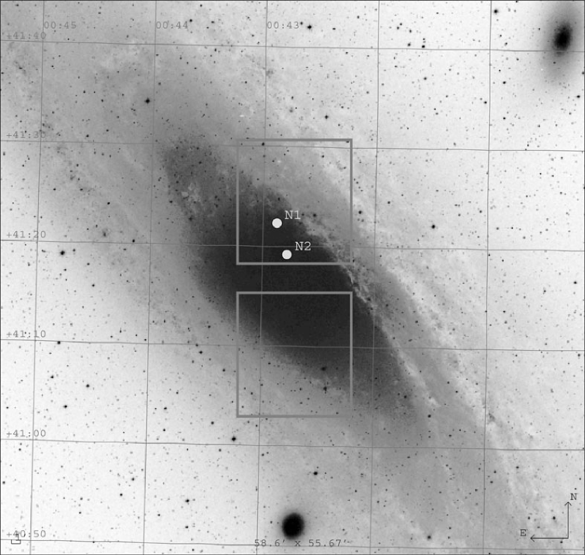
Figure 4.— Projected on M31, we display the boundaries of the two 13’x12.6’ monitored fields. The filled circle mark the position of the selected microlensing candidate events.

Table 3Characteristics of the microlensing candidates OAB-N1 and OAB-N2.

	OAB-N1	OAB-N2
		OAB data	source flux fixed
$\alpha$ (J2000)	0h 42m 57s	0h 42m 50s
$\delta$ (J2000)	$41^{\circ}22^{\prime}50^{\prime\prime}$	$41^{\circ}18^{\prime}40^{\prime\prime}$
$d_{\mathrm{M}31}$ (arcmin)	7.1	2.8
$t_{0}$ (JD-2450000.0)	$4433.8\pm 0.2$	$4467.3_{-1.3}$	$4466.6\pm 0.3$
$t_{1/2}$ (days)	$7.1^{+1.4}_{-1.3}$	$2.6^{+1.0}_{-0.5}$	$2.56^{+0.12}_{-0.20}$
$\Delta R$	$21.1\pm 0.2$	$19.1^{+0.8}$	$19.5\pm 0.2$
$R-I$	$1.0\pm 0.2$	$1.1\pm 0.1$	1.2
$\chi^{2}/\mathrm{dof}$	3.9	1.4	1.1
$t_{\mathrm{E}}$ (days)		$3.9^{+2.7}$	$4.18^{+0.55}_{-0.41}$
$u_{0}$		$0.23_{-0.12}$	$0.224^{+0.008}_{-0.029}$
$\phi^{*}_{R}$ (ADU s-1)		$15_{-12}$	$7.6$
$\phi^{*}_{I}$ (ADU s-1)		$28_{-22}$	$15.1$
$R^{*}$		$20.2^{+1.4}$	$20.9$
$I^{*}$		$19.1^{+1.7}$	$19.7$

Note. — For OAB-N2, we show the results for the fit performed both with our data set alone (left column) and fixing the source flux from a possible identification with a source in the Massey et al. (2006) catalogue. The error on the standard magnitude values and colors includes an extra $\pm 0.1~{}\mathrm{mag}$ term from the calibration equation.

The selection pipeline described in the previous section leaves us with two candidate microlensing events, which we name OAB-N1 and OAB-N2 (“N” indicates that they are both located in our “North” field). Their characteristics are summarised in Table 3, and their position within our field of view is shown in Fig. 4. As for the sampling criterion, OAB-N1 fulfills both sets A and B demands, while OAB-N2 only the set B one.

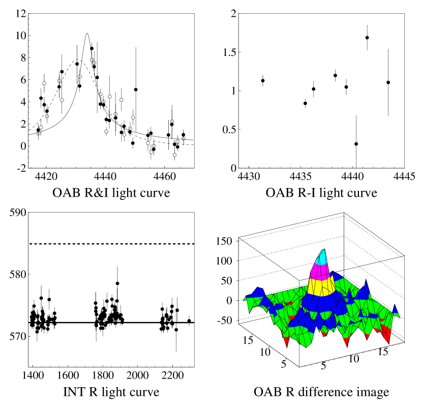
Figure 5.— The microlensing candidate event OAB-N1. Top left panel: $R$ and $I$-band light curves (filled and empty symbols, respectively). The $R$-band data are normalized with respect to $I$-band data using the color of the flux variation. The solid and the dashed lines are the best-fitting Paczyński curves with $t_{0}=4433.8$ and $t_{0}=4430.6$ (JD-2450000.0), respectively (Sect. 5.2 for details). Top right panel: color light curve. Bottom panel (left): the extension along the INT data (the solid and dotted lines are as in Fig. 3). The units on the $x$ axes are time in days (JD-2450000.0). The ordinate axes units are flux in ADU s^-1 per superpixel (left panels) and magnitude (top right panel). Bottom panel right: OAB $R$-band data surface plot image difference between the image at maximum magnification and the baseline level. The units on the space $x-y$ axes is pixels, the surface plot values are in ADU per pixel.

OAB-N1 : This is a relatively large flux variation, with significance bump estimators equal to $L=183$ and $Q=108$; quite short, $t_{1/2}=7.1~{}\mathrm{days}$, and not too bright, $\Delta R=21.1$. The OAB-N1 light curve is shown in Fig. 5, together with its INT extension and the image difference around the candidate position upon which is based our PSF analysis. The INT data extension of the OAB-N1 light curve appears to be flat (small Lomb periodogram power, $P_{R}=6.3$, and significantly large value for the difference of flux deviation, $\delta(\Delta f)=10.0$). However, the quality of the Paczyński fit is not good. A few points before the bump deviate significantly from the expected shape, and this is reflected in the rather poor value of $\chi^{2}$. This might be attributed to underlying nearby variables, but we can not exclude it to be a sign of an intrinsic non-microlensing nature. Indeed, we have shown that OAB-N1 is located in a part of the $t_{1/2}-\Delta R$ parameter space where the background of variable stars is large (top panel, Fig. 2). A possible contamination, compatible with its “one bump” nature, besides a possible very long period variable, might come from some kind of eruptive variable (even if Novæ can be excluded because the flux variation is far too small). On the other hand, the descent is fairly well sampled and matches nicely enough the fitted Paczyński shape. In the top right part of Fig. 5 we show the “color” light curve, namely the ratio $R$ over $I$ band of the difference of the light curve flux, along the bump, and the background level, that we expect to be constant for microlensing.

Through the pipeline, and in particular for OAB-N1, as an initial condition for the time of maximum magnification in the Paczyński fit we choose the value of the time corresponding to the data point with the maximum flux value, in this case $t=4435.4$ (JD-2450000.0). During the fit procedure it is difficult for this parameter to exit from the $\chi^{2}$ minimum well around this value (whose bounds are usually set by the sampling) and indeed as a result we find $t_{0}=4433.8\pm 0.2$ (JD-2450000.0). Motivated by the OAB-N1 light curve appearance, irregular sampling and noisy aspect, we have therefore carried out a search for other $\chi^{2}$ minima in different regions of the $t_{0}$ space. As a result we have found a new, well isolated, minimum with a lower value of the reduced $\chi^{2}$ ($\chi^{2}/\mathrm{dof}=3.5$ to be compared with $\chi^{2}/\mathrm{dof}=3.9$ found in the previous case) for $t_{0}=4430.6\pm 0.4$ (JD-2450000.0). Correspondingly, we find new values for the duration and the flux deviation at maximum, $t_{1/2}=18~{}\mathrm{days}$ and $\Delta R=21.5$ (this last value being at the limit of our threshold cut), namely, a rather different result from the previous one. Such a light curve would have still been selected as a microlensing candidate within our pipeline. However, the longer duration would have futher weakened its microlensing interpretation (Sect. 5.4). The co-existence of these two minima might be suggestive, accepting the microlensing hypothesis, of a binary lens or binary source solution. The available data, however, do not allow us to robustly test this hypothesis.

Figure 6.— The microlensing candidate event OAB-N2. Top panel: normalized $R$ and $I$-band light curves (filled and empty symbols, respectively). The $R$-band data are normalized with respect to $I$-band data using the color of the flux variation. The solid line is the best-fitting Paczyński curve. In the insert we show the residual with respect to the Paczyński fit along the bump. Bottom panels, left: color light curve; right: extension along the INT data (the solid and dotted lines are as in Fig. 3). The units on the $x$ axes are time in days (JD-2450000.0). The ordinate axes units are magnitude for the bottom left panel, and flux in ADU s^-1 per superpixel for the remaining panels.

OAB-N2 : This looks (Fig. 6) like an extremely bright and short flux variation ($t_{1/2}=2.6~{}\mathrm{days}$, $\Delta R=19.1$), located near the M31 center (at a distance $d=2.8^{\prime}$), with a completely flat INT extension ($P_{R}=8$, $\delta(\Delta f)=25$). The sampling along the bump is, however, extremely poor (indeed, both the time of maximum amplification and the flux deviation at maximum are not strongly constrained, Table 3). In particular, the lack of data points in the descent prevents us from probing the expected microlensing symmetric shape, so that it is difficult to draw definitive conclusions about its nature. On the other hand, the rising part of OAB-N2 looks achromatic, and is rather well constrained, and this strengthens the microlensing hypothesis. Indeed, both the shape and the achromaticity are hardly compatible with the only possible kind of contamination for such a kind of flux variation, if not microlensing, namely some sort of eruptive-like object. Furthermore, though few, the points along the bump allow us to get to a reasonable fit for all the parameters of the microlensing event. At the $1~{}\sigma$ level, the $\chi^{2}$ analysis gives us best values and lower bounds for the impact parameter and the source flux and best value and upper bound for the Einstein time (with, however, a rather large relative $1~{}\sigma$ error, even exceeding 50%, Table 3). Finally, the guess for the flux source value allows us to carry out a more constrained color analysis (as for OAB-N1, but subtracting the source flux from the baseline, bottom left panel of Fig. 6). As for the value of the source flux, the results of the Paczyński fit have been confirmed by the cross-identification of the possible source star in the catalogue of Massey et al. (2006). Indeed, within 1 pixel of our evaluated position, we find a typical red giant with $R_{C}=20.9$ and $R-I=1.2$ (values fully compatible with those evaluated from our data set alone). The knowledge of the source flux allows us to better constrain the fit parameters, in particular the time of maximum amplification and the flux deviation at maximum (in fact $t_{0}$ shifts back to the position of the last observed data-point so that, accordingly, $\Delta R$ gets fainter). Furthermore, we may now completely break the degeneracy among the amplification parameters. Indeed, we estimate $t_{\mathrm{E}}=4.2^{+0.6}_{-0.4}$ days and $u_{0}=0.22^{+0.01}_{-0.03}$ ($A_{\mathrm{max}}=4.5$).

We have also searched for $X$-ray counterparts in the XMM-Newton archive and verified that neither of the microlensing candidates’ coordinates correspond to any of the identified sources in the EPIC images (Strüder et al., 2001; Turner et al., 2001; Shirey et al., 2001). In the case of OAB-N2 there is an $X$-ray counterpart, but only within $\sim 30^{\prime\prime}$, so that we can safely rule out the identification.

5.3. The expected number of events

Table 4The expected number of microlensing events.

	$n_{\mathrm{exp}}$
	set A	set B
bulge-bulge	$0.35\pm 0.07$	$0.44\pm 0.08$
bulge-disk	$0.18\pm 0.02$	$0.23\pm 0.03$
disk-bulge	$0.06\pm 0.01$	$0.07\pm 0.01$
disk-disk	$0.015\pm 0.002$	$0.019\pm 0.002$
SL	$0.6\pm 0.1$	$0.8\pm 0.1$
mass ($\mathrm{M}_{\odot}$)
1	$0.7\pm 0.1$	$0.9\pm 0.2$
0.5	$1.1\pm 0.2$	$1.3\pm 0.2$
0.1	$1.6\pm 0.1$	$1.9\pm 0.1$
$10^{-2}$	$2.0\pm 0.2$	$2.3\pm 0.2$
$10^{-3}$	$1.3\pm 0.2$	$1.5\pm 0.2$

Note. — The expected number of microlensing events, for M31 self lensing (lenses belonging to either the M31 bulge or disk) and MACHO lensing (lenses belonging to either the M31 or the Milky Way halo), for a full halo with different values of the MACHO mass. For self-lensing events we report also the number for each lens-source population we consider. We report the results of the Monte Carlo simulation corrected for the efficiency evaluated according to both set A and B criteria.

The Monte Carlo simulation, completed by the efficiency analysis, allows us to estimate the expected number of microlensing events for our experimental setup. In Table 4 we report the resulting values, already corrected for the efficiency. The results we obtain using the set B criteria is larger by up to about 30% with respect to set A. This is a combined effect of the larger value of the efficiency and of the effective baseline length increase.

As for self-lensing events, it turns out that most of them, $\sim 50\%$, are due to bulge-bulge events (lens-source, respectively), with the remaining distributed almost equally between disk-bulge and bulge-disk events. The second configuration is enhanced in the South field because in this case we see the bulge in front of the disk. It is also worth noting that, according to our model, almost half of the overall bulge mass is located within our cone of view, but only about 1/7 of that of the M31 disk.

As for MACHO lensing, about 2/3 of the events are expected to belong to the M31 halo. Actually, the overall mass within our cone of view of the M31 halo is larger than the Galactic one by a factor of a few thousands, but Milky Way halo lensing is strongly enhanced by the much larger size of the Einstein radius. We expect the largest number of MACHO lensing events from $10^{-1}-10^{-2}~{}\mathrm{M}_{\odot}$ objects, as our efficiency drammatically drops for smaller MACHO masses.

Together with the expected event number we report the statistical error associated with the simulation on the basis of Poisson statistics. The uncertainties intrinsic in the model (whose detailed discussion is beyond the scope of the present paper) make, however, the corresponding systematic error in principle even larger.

5.4. Discussion

We have designed our (fully automated) pipeline so as to get rid of most forms of stellar variability, while preserving genuine microlensing. As a result, therefore, all survivors could in principle be variables but with varying (hopefully large) degrees of confidence that they are not. Coming to the present data set, we have selected two flux variations compatible with a microlensing signal. While discussing the possible physical meaning of this result, however, we have to keep in mind that, although with different degrees of confidence, we have no strong evidence in favour of the microlensing hypothesis for either candidate: OAB-N1 because of both the light curve appearance (reflected in the $\chi^{2}$ value) and its position in the duration/flux-deviation parameter space, and OAB-N2 because of its extremely poor sampling (that has not prevented us, however, from finding a convincing microlensing Paczyński fit further confirmed by the possible identification of the source). In conclusion, looking at the candidate light curves, we might be tempted to classify OAB-N1 as a very “poor” candidate, and OAB-N2 as a “good” one, keeping in mind, however, that this might simply reflect the bias induced by the observational sampling.

With the care suggested by the above discussion, we come now to the comparison of the observed events with the expected signal. As for the event characteristics we may take as a reference the distributions shown in Fig. 1. Given the caveat that these distributions can not be compared directly with the results of the analysis because of the correlation of the pipeline efficiency with the event characteristics, both candidates appear compatible with the expected signal with respect to the duration and the distance from the M31 center (being both shorter and nearer to the M31 center, OAB-N2 appears, also in this respect, a stronger candidate than OAB-N1). Coming to the number of events, we must compare our observed candidates with the results reported in Table 4. First, we are bound to consider the case that MACHO lensing does not contribute at all, so that we are left with the expected lensing signal from the luminous populations alone, with an expected number of events for self-lensing somewhat smaller than 1. Even allowing for both our candidates to be genuine microlensing, this is still, according to Poisson statistic, fully compatible with the observations.

On the other hand, the expected number of MACHO lensing events is not large if compared to that of self lensing. Even for a full MACHO halo we would expect about as many self-lensing events as MACHO lensing. It is clear, therefore, that on the basis of the number of events alone our statistics are still too small to draw conclusions on this contribution.

It may be asked, then, how we might disentangle the two signals: self lensing from MACHO lensing. First, an improvement in the event statistics might help us to further exploit the expected differences in the spatial distributions (top panels, Fig. 1). Second, a good enough sampling (such as was not the case for the present selection) might allow a sufficient characterisation of the selected flux variations. In turn, this could give possible hints on the nature of the lens, as was the case for the detailed analysis linked to the finite source size effect for the PA-S3 event carried out by Riffeser et al. (2008). Both these reasons motivate the need for further observations.

6. Conclusions

In this paper we have presented a thorough analysis of the data acquired during the second season of our pixel-lensing observational campaign carried out towards M31 with the $152~{}\mathrm{cm}$ Cassini telescope located in Loiano. We have developed a fully automated pipeline analysis for the detection and the characterisation of Paczyński like microlensing flux variations. We have evaluated, through a Monte Carlo simulation, the expected signal, given an astrophysical model for M31 and the efficiency of our pipeline. As a result we have selected 1-2 candidate microlensing events. This output turns out to be in fair agreement with our evaluation of the expected self-lensing signal from the luminous M31 components. As for the would-be MACHO lensing signal, the statistics of events are still too small to draw firm conclusions. Further observations might help us to disentangle between the two populations. First, because of the larger statistics of events, second (provided a better sampling) because of a better characterisation of the light curves.

Previous analyses, in particular those carried out using data collected at the INT telescope by the POINT-AGAPE and the MEGA collaborations, have reached different conclusions on the dark matter halo content in the form of MACHOs along the line of sight towards M31 (Calchi Novati et al., 2005; de Jong et al., 2006). Their fundamental point of disagreement may be traced back to the evaluation of the expected self-lensing signal. In this perspective our campaign, as well as that carried out by the ANGSTROM collaboration right towards the M31 center (Kerins et al., 2006), may help in shedding more light onto this important issue.

Appendix A The microlensing pipeline: the sampling criterion

The rationale of the present cut is to test whether the detected flux variation is sufficiently sampled. As a starting point we use the results of the Paczyński fit, and in particular the values of the time at maximum magnification, $t_{0}$, and of the bump duration, the full-width-at-half-maximum $t_{1/2}$. Given these values we identify six intervals along the light curve, symmetric around $t_{0}$, $[t<t_{0}-3~{}t_{1/2}]$, $[t_{0}-3~{}t_{1/2}<t<t_{0}-t_{1/2}/2]$, $[t_{0}-t_{1/2}/2<t<t_{0}]$, $[t_{0}<t<t_{0}+t_{1/2}/2]$, $[t_{0}+t_{1/2}/2<t<t_{0}+3~{}t_{1/2}]$ and $[t>t_{0}+3~{}t_{1/2}]$.

As a first set of criteria we ask for at least $n_{\mathrm{min}}$ data-points in at least 3 out of the 4 inner intervals, within $t_{0}\pm 3~{}t_{1/2}$, and at least 1 data-point in both the joined outer intervals $t<t_{0}-t_{1/2}/2$ and $t>t_{0}+t_{1/2}/2$, namely, we allow the same data-point to be counted twice. The value of $n_{\mathrm{min}}$ is fixed according to the duration, with $n_{\mathrm{min}}=1,2,3$ for $t_{1/2}<5,<15,>15~{}\mathrm{days}$, respectively.

As a second set of criteria we ask for at least 1 data-point in at least 2 out of the 4 inner intervals and at least 1 data-point in at least 1 of the two tail intervals ($t<t_{0}-3~{}t_{1/2}$ and $t>t_{0}+3~{}t_{1/2}$).

We refer to the two set of criteria, and to the corresponding selected flux variations, as set “A” and set “B”, respectively.

The set A criterion is more demanding as for the sampling along the inner part of the flux variation, whereas set B makes, in a way, a stronger demand on the coverage of the far tails, so that set A selected events are not a simple subsample of set B events. Furthermore, it results that the time of maximum magnification for set A events is constrained within the limits of the observational run whereas for set B it can also fall (slightly) outside. Set B flux variations therefore enjoy an effective longer baseline.

The sampling analysis is carried out along $R$-band data only.

Appendix B The microlensing pipeline: the PSF criterion

As outlined in Sect. 3, through this criterion we want to check whether the detected variation along the light curve can be attributed to a physically meaningful flux variation (a variable star or microlensing) or to some kind of spurious signal (cosmic rays, bad pixel, seeing effects and so on). To this purpose we have to turn to an analysis carried out on the images. As a criterion we test whether the spatial form of the detected bump has a well enough shaped PSF. As we are not carrying out difference image photometry, we can safely stop at the first order approximation of a 2-dimensional Gaussian, namely

$$P(x,y)=\exp\Bigg{\{}-\frac{1}{2(1-\rho^{2})}\Bigg{[}\left(\frac{x-\mu_{x}}{\sigma_{x}}\right)^{2}+\left(\frac{y-\mu_{y}}{\sigma_{y}}\right)^{2}-2\rho\left(\frac{x-\mu_{x}}{\sigma_{x}}\right)\left(\frac{y-\mu_{y}}{\sigma_{y}}\right)\Bigg{]}\Bigg{\}}\,.$$ (B1)

We carry out this analysis on a difference image (a window of 19x19 pixels around the central pixel $x_{0},y_{0}$ in which the flux variation has been detected) built as follows. Given the time of maximum magnification of the bump variation, $t_{0}$, we look for the nearest night of observation, and we average the images collected during this night, taking note of the average seeing of the night. As a baseline image we take the average of a set of images chosen along the baseline with a similar seeing.

As a criterion, we ask for the fit with respect to the 2-dimensional Gaussian to converge “properly”. Besides the actual demand for the fit to converge we also ask the following : $|x_{0}-\mu_{x}|<1.5$, $|y_{0}-\mu_{y}|<1.5$, $1<\sigma_{x}<3$, $1<\sigma_{y}<3$ and $|\rho|<0.5$. This additional set of criteria is necessary as it is very easy, in case of spurious variations, for the fit to converge while it slips at the border of the physically meaningful bounds.

It is worth noticing that a different parametrisation for the 2-d Gaussian profile with respect to that chosen in Eq. B1 is sometime used, namely

$$P_{1}(x,y)=\exp\Bigg{[}-\frac{(x\cos\phi+y\sin\phi)^{2}}{2\sigma_{a}^{2}}-\frac{(x\sin\phi-y\cos\phi)^{2}}{2\sigma_{b}^{2}}\Bigg{]}\,.$$ (B2)

In fact the two formulations are equivalent, one can easily evaluate the parameters $\sigma_{a},\,\sigma_{b}$ and $\phi$ as a function of $\sigma_{x},\,\sigma_{y}$ and $\rho$, and vice versa (it must be noted, however, that the parameter $\rho$ plays a double role, giving both an inclination and a distortion). Within the parametrisation of Eq. B2 we find our cuts to roughly correspond to $1<\sigma_{a}<3$, $1<\sigma_{b}<3$, and $\phi\approx\mathrm{arbitrary}$. Still, we prefer Eq. B1 as the fit procedure looks, in this case, more stable.

Appendix C Monte Carlo simulation: the drawing process

In this Appendix we discuss some further details regarding the Monte Carlo simulation described in Sect. 4.

A microlensing event is fully specified by 10 parameters. The line of sight, specified by two angles, $\theta,\rho$, out of which we determine the (angular) position within our fields as $x=\rho\cos(\theta),y=\rho\sin(\theta)$; the lens distance $D_{l}$ and mass $\mu_{l}$; the source distance $D_{s}$ and flux $\phi_{s}$; the lens-source relative velocity, specified by a modulus $v_{r}$ and a phase $\psi_{v}$; finally the microlensing amplification parameters, the impact parameter $u_{0}$ and the time of maximum amplification $t_{0}$. Each of these parameters has its own physical distribution function from which we draw a value for each event realisation. Even if we simulate only $R$ light curves, the available information within the luminosity functions used allows us to evaluate also the source radius, so to properly take into account the finite size source effect, as for the microlensing amplification.

A key aspect of our Monte Carlo scheme is the “weight”, $w_{i}$, that we associate to each event. This is linked in part to the drawing process and in part to the physical process we are studying. As for the first part, this follows from the fact that for a given distribution function we have two choices as for the drawing process. Either we may directly draw according to the distribution, and in this case the corresponding weight is $w_{i}=1$, either we may draw with a uniform distribution and give the event a weight proportional to the distribution function. As for the second part, we take the weight to be proportional to the following

$$w_{i}\propto\left(2\,R_{\mathrm{E}}\,u_{\mathrm{MAX}}\,v_{r}\,\Delta T_{\mathrm{OBS}}\right)\times n_{s}\,,$$ (C1)

where $R_{\mathrm{E}}$ is the Einstein radius, $u_{\mathrm{MAX}}$ the maximum value for the impact parameter, $\Delta T_{\mathrm{OBS}}$ the duration of the observational campaign, $n_{s}$ the number surface density of available sources (fox a fixed line of sight). In fact, according to our simulation scheme, first we fix the lens line of sight and specify all of the events characteritics. Then , as the purpose of the Monte Carlo is to evaluate the number of expected microlensing events, we have to evaluate how many sources (given the M31 surface brightness and luminosity function) are available within a surface delimited by the event characteristics and the experimental conditions. Indeed, the term $2\,R_{\mathrm{E}}\,u_{\mathrm{MAX}}\,v_{r}\,\Delta T_{\mathrm{OBS}}$ in Eq. C1 is the surface area on the lens plane (for a fixed event configuration) where it is possible to find a suitable source.

The last contribution to the weight comes from the need to evaluate the number of available lenses. For each lens population this is computed as the ratio of the total mass of the component within the observed field of view divided by the average lens mass. More specifically, the weight linked to the choice of the line of sight is normalized to the total mass.

As for the drawing of the line of sight we have the following: for lenses in the Milky Way halo we assume the spatial distribution across the observed field of view to be uniform; for lenses in the M31 halo, because of the assumed spherical symmetry, the resulting distribution for the angle $\theta$ is uniform; for bulge and disk lenses we make use of the Kent (1989) bulge-disk decomposition (whenever using the Kent (1989) profile we use a uniform distribution and then attribute to the event a “weight” as described above).

Once the event configuration, and its weight, have been specified, we build the corresponding light curve and, given our observational set up, we evaluate whether the event is selected or not. This selection process is completely independent of the event weight. The selected events delimit the overall integration space, so that the expected number of events is given by the sum of the weights of these selected events only. (This same set of events is then taken, with all of their characteristics, as the input set for the simulation on the images described in Sect. 4.2.)

In Table 5 we report, for each parameter, the distribution function used and its range of variability.

Table 5Monte Carlo parameters: distributions function and limits for each lens/source population.

	MW halo	M31 halo	M31 bulge	M31 disk
					limit
$\theta$	uniform	uniform	K89	K89+$f(\zeta)$	field of view
$\rho$	uniform	$\rho_{\mathrm{HM31}}(\vec{r})$	K89	K89+$f(\zeta)$	field of view
$D_{l}$	$\rho_{\mathrm{HMW}}(\vec{r})$	$\rho_{\mathrm{HM31}}(\vec{r})$	K89	K89+$f(\zeta)$	model
$\mu_{l}$	$\delta(\mu_{l})$	$\delta(\mu_{l})$	$\mu^{-\alpha}$	$\mu^{-\alpha}$	model
$D_{s}$	-	-	K89	K89+$f(\zeta)$	model
$\phi_{s}$	-	-	IAC	Hipparcos	$M_{I}<2$
$v_{r}$	Gaussian	Gaussian	Gaussian	Gaussian	$0,\infty$
$\psi_{v}$	uniform	uniform	uniform	uniform	$0,2\pi$
$u_{0}$	uniform	uniform	uniform	uniform	$0,u_{\mathrm{MAX}}(=2)$
$t_{0}$	uniform	uniform	uniform	uniform	$0,\Delta T_{\mathrm{obs}}$

Note. — The parameters have been introduced in Appendix C. The details for the density function of the Milky Way and the M31 halos and for the source luminosity functions are given in Sect. 4.1. K89 stands for the Kent (1989) bulge-disk decomposition. For the disk, as only a two-dimensional distribution on the plane is given, we consider a vertical distribution $f(\zeta)=\mathrm{cosh}(-(\zeta/\zeta_{h}))^{2}$, where $\zeta_{h}$ is the vertical scale height. The index for the power law mass function are given in Sect. 4.1. In the last column we report the range of variability for each parameter: for $\theta,\rho$ “field of view” indicates the two observed fields, “Nord” and “Sud” (Sect. 2.1); for the distances we take the physical boundaries of the component considered, in particular for the halos we use a truncation radius as specified in Sect. 4.1, for the bulge $\sim~{}7~{}\mathrm{kpc}$ around the M31 distance while for the disk vertical component we draw directly from the given distribution (for a fixed line of sight this allows us to evaluate the physical distances); for bulge and disk lenses $\mu_{l}$ is drawn with a lower limit of $0.08~{}\mathrm{M}_{\odot}$ and upper limit of $1.0~{}\mathrm{M}_{\odot}$ and $10.0~{}\mathrm{M}_{\odot}$, respectively.

References

- Alcock et al. (2000) Alcock, C., et al. 2000, ApJ, 542, 281
- Ansari et al. (1999) Ansari, R., et al. 1999, A&A, 344, L49
- Ansari et al. (1997) Ansari, R., et al. 1997, A&A, 324, 843
- Aparicio & Gallart (2004) Aparicio, A., & Gallart, C. 2004, AJ, 128, 1465
- Aurière et al. (2001) Aurière, M., et al. 2001, ApJ, 553, L137
- Baillon et al. (1993) Baillon, P., Bouquet, A., Giraud-Heraud, Y., & Kaplan, J. 1993, A&A, 277, 1
- Baltz et al. (2004) Baltz, E. A., Lauer, T. R., Zurek, D. R., Gondolo, P., Shara, M. M., Silk, J., & Zepf, S. E. 2004, ApJ, 610, 691
- Bennett (2005) Bennett, D. P. 2005, ApJ, 633, 906
- Bozza et al. (2008) Bozza, V., Calchi Novati, S., & Mancini, L. 2008, ApJ, 675, 340
- Bozza et al. (2009) Bozza, V., et al. 2009, in preparation
- Calchi Novati et al. (2007) Calchi Novati, S., et al. 2007, A&A, 469, 115
- Calchi Novati et al. (2006) Calchi Novati, S., De Luca, F., Jetzer, P., & Scarpetta, G. 2006, A&A, 459, 407
- Calchi Novati et al. (2002) Calchi Novati, S., et al. 2002, A&A, 381, 848
- Calchi Novati et al. (2003) Calchi Novati, S., Jetzer, P., Scarpetta, G., Giraud-Héraud, Y., Kaplan, J., Paulin-Henriksson, S., & Gould, A. 2003, A&A, 405, 851
- Calchi Novati et al. (2005) Calchi Novati, S., et al. 2005, A&A, 443, 911
- Carignan et al. (2006) Carignan, C., Chemin, L., Huchtmeier, W. K., & Lockman, F. J. 2006, ApJ, 641, L109
- Crotts (1992) Crotts, A. P. S. 1992, ApJ, 399, L43
- Crotts & Tomaney (1996) Crotts, A. P. S., & Tomaney, A. B. 1996, ApJ, 473, L87
- de Jong et al. (2004) de Jong, J. T. A., et al. 2004, A&A, 417, 461
- de Jong et al. (2006) de Jong, J. T. A., et al. 2006, A&A, 446, 855
- Evans & Belokurov (2006) Evans, N. W., & Belokurov, V. 2006, MNRAS, 1281
- Gould (1996) Gould, A. 1996, ApJ, 470, 201
- Han (1996) Han, C. 1996, ApJ, 472, 108
- Jahreiß & Wielen (1997) Jahreiß, H., & Wielen, R. 1997, in ESA Special Publication, Vol. 402, Hipparcos - Venice ’97, 675
- Jetzer (1994) Jetzer, P. 1994, A&A, 286, 426
- Joshi et al. (2005) Joshi, Y. C., Pandey, A. K., Narasimha, D., & Sagar, R. 2005, A&A, 433, 787
- Kent (1989) Kent, S. M. 1989, AJ, 97, 1614
- Kerins et al. (2001) Kerins, E., et al. 2001, MNRAS, 323, 13
- Kerins et al. (2006) Kerins, E., Darnley, M. J., Duke, J. P., Gould, A., Han, C., Jeon, Y.-B., Newsam, A., & Park, B.-G. 2006, MNRAS, 365, 1099
- Kroupa (2007) Kroupa, P. 2007, ArXiv Astrophysics e-prints, astro-ph/0703124
- Mancini et al. (2004) Mancini, L., Calchi Novati, S., Jetzer, P., & Scarpetta, G. 2004, A&A, 427, 61
- Massey et al. (2006) Massey, P., Olsen, K. A. G., Hodge, P. W., Strong, S. B., Jacoby, G. H., Schlingman, W., & Smith, R. C. 2006, AJ, 131, 2478
- Murdin (2001) Murdin, P. 2001, Encyclopedia of astronomy and astrophysics (Encyclopedia of Astronomy and Astrophysics)
- Paczyński (1986) Paczyński, B. 1986, ApJ, 304, 1
- Paulin-Henriksson et al. (2003) Paulin-Henriksson, S., et al. 2003, A&A, 405, 15
- Perryman et al. (1997) Perryman, M. A. C., et al. 1997, A&A, 323, L49
- Press et al. (1992) Press, W. H., Teukolsky, S. A., Vetterling, W. T., & Flannery, B. P. 1992, Numerical recipes in FORTRAN. The art of scientific computing (Cambridge: University Press, —c1992, 2nd ed.)
- Riffeser et al. (2003) Riffeser, A., Fliri, J., Bender, R., Seitz, S., & Gössl, C. A. 2003, ApJ, 599, L17
- Riffeser et al. (2006) Riffeser, A., Fliri, J., Seitz, S., & Bender, R. 2006, ApJS, 163, 225
- Riffeser et al. (2008) Riffeser, A., Seitz, S., & Bender, R. 2008, ApJ, 684, 1093
- Robin et al. (2003) Robin, A. C., Reylé, C., Derrière, S., & Picaud, S. 2003, A&A, 409, 523
- Sahu (1994) Sahu, K. C. 1994, Nature, 370, 275
- Sarajedini & Jablonka (2005) Sarajedini, A., & Jablonka, P. 2005, AJ, 130, 1627
- Schlegel et al. (1998) Schlegel, D. J., Finkbeiner, D. P., & Davis, M. 1998, ApJ, 500, 525
- Shirey et al. (2001) Shirey, R., et al. 2001, A&A, 365, L195
- Stephens et al. (2003) Stephens, A. W., et al. 2003, AJ, 125, 2473
- Strüder et al. (2001) Strüder, L., et al. 2001, A&A, 365, L18
- Tamm et al. (2007) Tamm, A., Tempel, E., & Tenjes, P. 2007, ArXiv:0707.4375
- Tisserand et al. (2007) Tisserand, P., et al. 2007, A&A, 469, 387
- Totani (2003) Totani, T. 2003, ApJ, 586, 735
- Turner et al. (2001) Turner, M. J. L., et al. 2001, A&A, 365, L27
- Vallenari et al. (2006) Vallenari, A., Pasetto, S., Bertelli, G., Chiosi, C., Spagna, A., & Lattanzi, M. 2006, A&A, 451, 125
- van der Marel & Guhathakurta (2008) van der Marel, R. P., & Guhathakurta, P. 2008, ApJ, 678, 187
- Walterbos & Kennicutt (1987) Walterbos, R. A. M., & Kennicutt, R. C., Jr. 1987, A&AS, 69, 311
- Witt & Mao (1994) Witt, H. J., & Mao, S. 1994, ApJ, 430, 505
- Wu (1994) Wu, X.-P. 1994, ApJ, 435, 66
- Xue et al. (2008) Xue, X. ., et al. 2008, ArXiv:0801.1232