Pair Distribution Function of One-dimensional “Hard Sphere” Fermi and Bose Systems

Abstract

The pair distributions of one-dimensional “hard sphere” fermion and boson systems are exactly evaluated by introducing gap variables.

I Introduction

Recent experimental progress in one-dimensional (1D) systems renews theoretical interest in such systems. In this paper we study the pair distribution function in 1D “hard sphere” systems.

Pair distribution function in 1D Tonks gas Tonks and Lieb-Liniger Bose gas Lieb1 ; Lieb2 have been studied previously, including the local correlation, $D(0)$, asymptotic properties at large $r$, and the zero temperature behaviorufford ; Girardeau60 ; Girardeau65 ; Castin ; Gangardt ; Kheruntsyan1 ; Drummond ; Astrakhsrchick ; Cherny ; Kheruntsyan2 . The pair distribution function for 3D hard sphere boson gas has been calculated by the authors bb . In this work we address the problem of pair distribution function in 1D hard sphere fermion and boson systems with the diameter of the particles $a\neq 0$.

The pair distribution function is defined as

$$D(r_{12}) = \rho^{-2}\langle\psi^{{\dagger}}(\textbf{r}_{1})\psi^{{\dagger}}(\textbf{r}_{2})\psi(\textbf{r}_{2})\psi(\textbf{r}_{1})\rangle$$ (1)

where $\rho=N/L$ is the density. $D(r)$ is an important physical quantity measurable for many liquid systems. In this formula $\psi(\textbf{r})$ is the annihilation operator in r space.

The pair distribution function $D(r_{12})$ is also related to the diagonal elements of the reduced density matrix cnyang :

$$D(r_{12})=\rho^{-2}\text{Tr}[\psi(\textbf{r}_{2})\psi(\textbf{r}_{1})\rho_{N}\psi^{{\dagger}}(\textbf{r}_{1})\psi^{{\dagger}}(\textbf{r}_{2})],$$ (2)

where $\rho_{N}=\Psi_{0}\Psi_{0}^{{\dagger}}$, and $\Psi_{0}$ is the many body wave function.

The meaning of $D(r)$ is: given a particle A at one point, the probability of finding another particle B at distance $r$ (counterclockwise) is

$$\rho D(r)dr.$$ (3)

It is obvious that $D(r)\rightarrow 1$ as $r\rightarrow\infty$. also

$$\int_{0}^{L}\rho D(r)dr=N-1.$$ (4)

II Fermions with $a=0$

II.1 Wave Function $\Psi$ For Fermions With $a=0$

First, we consider $N$ free fermions in a one-dimensional cyclic interval of length $L$. The momenta of these fermions are $2\pi k/L$, where $k=-(N-1)/2$ to $(N-1)/2$. Here we consider the case that the number of fermions in the system is odd, $N=2n+1$. The normalized many body wave function $\Psi(r_{1},r_{2},\cdots,r_{N})$ of the system is of the form

$$\Psi=\frac{1}{\sqrt{N!}}\det\begin{pmatrix}\epsilon_{1}^{n}&\epsilon_{2}^{n}&\ldots&&\epsilon_{2n+1}^{n}\\ \epsilon_{1}^{n-1}&\epsilon_{2}^{n-1}&\ldots&&\epsilon_{2n+1}^{n-1}\\ \epsilon_{1}^{n-2}&\epsilon_{2}^{n-2}&\ldots&&\epsilon_{2n+1}^{n-2}\\ \vdots&\vdots&\ddots&&\vdots\\ \epsilon_{1}^{-n}&\epsilon_{2}^{-n}&\ldots&&\epsilon_{2n+1}^{-n}\end{pmatrix}$$ (5)

where $\epsilon_{j}=\text{exp}({i\frac{2\pi}{L}r_{j}})/\sqrt{L}$. After some calculations, we arrive at a compact form for the wave function,

$$\Psi=\frac{1}{\sqrt{N!}}(\frac{1}{\sqrt{L}})^{N}[2^{N(N-1)/2}]\prod_{1\leq i<j\leq N}\sin[\frac{\pi}{L}(r_{j}-r_{i})]$$ (6)

The pair distribution function $D(r)$ for free fermions can be exactly obtained from this many-body wave function ufford

$$D(r)=1-\frac{\sin^{2}(\frac{N\pi r}{L})}{N^{2}\sin^{2}(\frac{\pi r}{L})}.$$ (7)

II.2 Gap Variables For Free Fermions

In order to prepare for dealing with the $a\neq 0$ problem, we introduce gap variables in the case $a=0$ as follows. Consider a region of the $N$ body $L\times L\times\cdots\times L$ coordinate system where, modulo $L$,

$$r_{1}\leq r_{2}\leq\cdots\leq r_{N}\leq r_{1}.$$ (8)

We shall designate this region as $R_{1}$. In this region, we introduce gap variables $\{g_{i}\}$ :

$$g_{i}=r_{i+1}-r_{i},\ \ i=1,2,3,\ldots,2n+1.$$ (9)

Obviously $\sum g_{i}=L$. With the gap variables the many body wave function $\Psi$ is given by

$$\Psi = Q[f(g_{1})f(g_{2})\cdots f(g_{2n+1})]$$

$$\times[f(g_{1}+g_{2})f(g_{2}+g_{3})\cdots f(g_{2n+1}+g_{1})]$$

$$\times[f(g_{1}+g_{2}+g_{3})\cdots f(g_{2n+1}+g_{1}+g_{2})]$$

$$\times\cdots\cdots$$

$$\times[f(g_{1}+\cdots+g_{n})\cdots f(g_{2n+1}+g_{1}+\cdots+g_{n-1})]$$

where $f(g)=\sin(\pi g/L)$, and $Q$ is the normalization factor given by

$$Q=\frac{1}{\sqrt{N!}}(\frac{1}{\sqrt{L}})^{N}[2^{N(N-1)/2}].$$ (11)

$\Psi$ has $(2n+1)\times n$ factors in total.

The probability distributions in $R_{1}$ is

$$|\Psi|^{2}dg_{1}dg_{2}\cdots dg_{N}\delta(\sum_{i=1}^{N}g_{i}-L)L$$ (12)

with all $g_{i}\geq 0$. Now $R_{1}$ is only one of the $(N-1)!$ regions of the full coordinate space. In each of these regions we have the same gap distribution as (12). Thus gap distribution probability $dP$ is

$$dP=(N-1)!L|\Psi|^{2}dg_{1}dg_{2}\cdots dg_{N}\delta(\sum_{i=1}^{N}g_{i}-L).$$ (13)

Figure 1: Cycle of length $L$.

II.3 Functions $F_{i}(r)$ For Free Fermions

We now evaluate the function $D(r)$ of expression (3) using (13). Going from particle A to B, counterclockwise in the cycle of length $L$, as shown in Fig. 1, there may be $i$ other particles, with $i=0,1,\cdots,(N-2)$. Thus

$$\rho D(r)=\rho[F_{0}(r)+F_{1}(r)+\cdots+F_{N-2}(r)],$$ (14)

where

$$\rho F_{i}(r)dr=\int\delta(\sum_{j=1}^{i+1}g_{j}-r)drdP$$ (15)

Thus

$$\rho F_{i}(r) = (N-1)!L\int|\Psi|^{2}\delta(\sum_{j=1}^{i+1}g_{j}-r)$$ (16)

$$\times \delta(\sum_{j=i+2}^{N}g_{j}-(L-r))dg_{1}dg_{2}\cdots dg_{N}$$

where all $g_{j}\geq 0$.

Integrating over $dr$ we get, from (15),

$$\int_{0}^{L}\rho F_{i}(r)dr=\int dP=1.$$ (17)

Thus by (14),$\int\rho D(r)dr=N-1$, confirming (4). Outside of the interval $(0,L)$ we define $F(r)$ by

$$F(r)=0\ \ \text{for}\ \ r<0\ \ \text{and}\ \ r>L.$$ (18)

Besides (17), $F_{i}(r)$ has also the following properties:
(i) It is analytic except at $r=0$ and $r=L$, where $F(r)$ and its first derivative are both zero.
(ii) $F_{i}(r)=F_{N-2-i}(L-r)$.

It is obvious from (16) that $NF_{i}(r)$ is a function of $N$ and $r/L$. In Fig. 2 we plot this function vs $r/L$ for the case $N=5$.

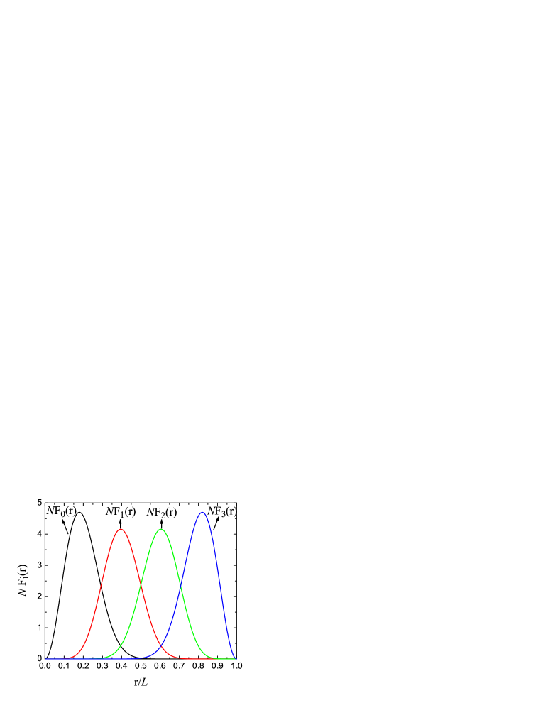
Figure 2: $NF_{i}(r)$ against $r/L$ for $N=5$ and $i=0,1,2,3$.

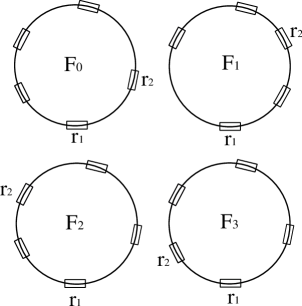
Figure 3: 4 possible configurations which contribute to the pair distribution function $D(r)$ for $N=5$. The ring represents the system and each block stands for a particle with diameter $a$.

Figure 4: Regions where $F_{i}(r)>0$ for $N=5$. Open circles are at $r=a,2a,3a,4a$. Closed circles are at $r=L-a,L-2a,L-3a$ and $L-4a$. These $2(N-1)=8$ circles are where $D(r)$ is singular. Each of the four regions has length $L-Na$.

III fermions with $a>0$

For fermions with $a>0$, the full coordinate space is again divided into $(N-1)!$ regions, one of which, $R_{1}$, is defined by the cyclic condition (8) modulo $L$. We introduce gap variables in $R_{1}$ by equations similar to (9):

$$g_{i} = r_{i+1}-r_{i}-a,\ \ i=1,2,3,\cdots,(N-1)$$ (19)

and $$g_{N}=r_{1}-r_{N}+L-a\hskip 93.89418pt(19a)$$

Obviously

$$\sum g=L-Na.$$ (20)

The key point is that $\Psi$ in terms of the gap variables $\{g\}$ is still given by (10), but with

$$f(g)=\sin(\pi g/(L-Na))$$ (21)

and

$$Q=\frac{1}{\sqrt{N!}}(\frac{1}{\sqrt{L-Na}})^{N}[2^{N(N-1)/2}].$$ (22)

Equation (12) now becomes

$$|\Psi|^{2}dg_{1}dg_{2}\cdots dg_{N}\delta(\sum_{i=1}^{N}g_{i}-(L-Na))L,$$ (23)

and (13) beomes

$$dP=(N-1)!L|\Psi|^{2}dg_{1}\cdots dg_{N}\delta(\sum_{i=1}^{N}g_{i}-(L-Na)).$$ (24)

The function $D(r)$ is again, as in (14), a sum of $(N-1)F$ functions. To illustrate the reasoning we turn to Fig. 3 and Fig. 4 for the case $N=5$. We have

$$D(r) = F_{0}[(r-a)\xi]+F_{1}[(r-2a)\xi]$$ (25)

$$+ F_{2}[(r-3a)\xi]+F_{3}[(r-4a)\xi],$$

where $\xi=L/(L-Na)$, and $F_{i}(r)$ is defined by (16) and (18).

Since $F_{i}(r)$ is nonzero only in the open interval $(0,L)$, for $N=5$,
$F_{0}[(r-a)\xi]$ is nonzero only for $a<r<L-4a$,
$F_{1}[(r-2a)\xi]$ is nonzero only for $2a<r<L-3a$,
$F_{2}[(r-3a)\xi]$ is nonzero only for $3a<r<L-2a$,
$F_{3}[(r-4a)\xi]$ is nonzero only for $4a<r<L-a$.
In Fig. 4 we indicate the regions where $F_{i}[(r-(i+1)a)\xi]$ is nonzero for $i=0$ to 3.

We present in Fig. 5 and Fig. 6 the function $D(r)$ for $N=5$, and for several values of $L/a$.

Returning now to the general case, we conclude

In the interval $(0,L)$, $D(r)$ is analytic everywhere except at $(N-1)$ open circles at $r=a,2a,\cdots,(N-1)a$, and at $(N-1)$ full circles at $r=L-a,L-2a,\cdots,L-(N-1)a$. At these singular points $D(r)$ is continuous and has a continuous first derivative.

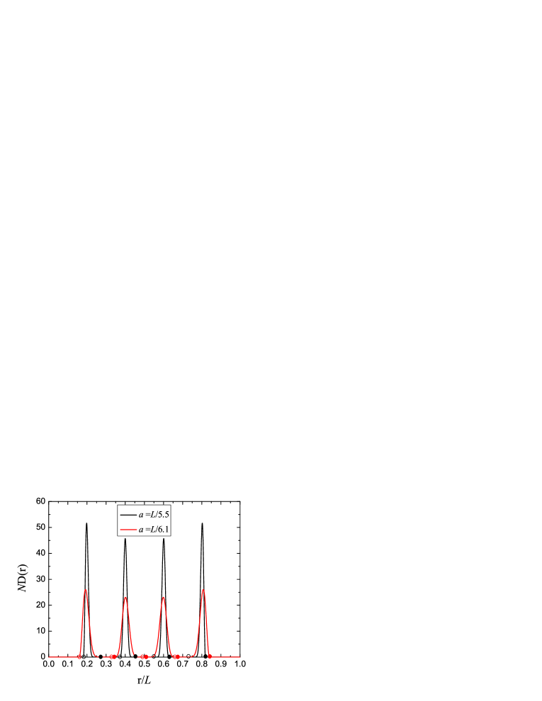
Figure 5: (color online) The pair distribution function $D(r)$ as a function of distance $r$ for $N=5$. The $N-1=4$ open circles and the $N-1=4$ closed circles are where $D(r)$ is singular.
     For case $a=L/(5+)$, $ND(r)$ is four $\delta$ functions (not shown).

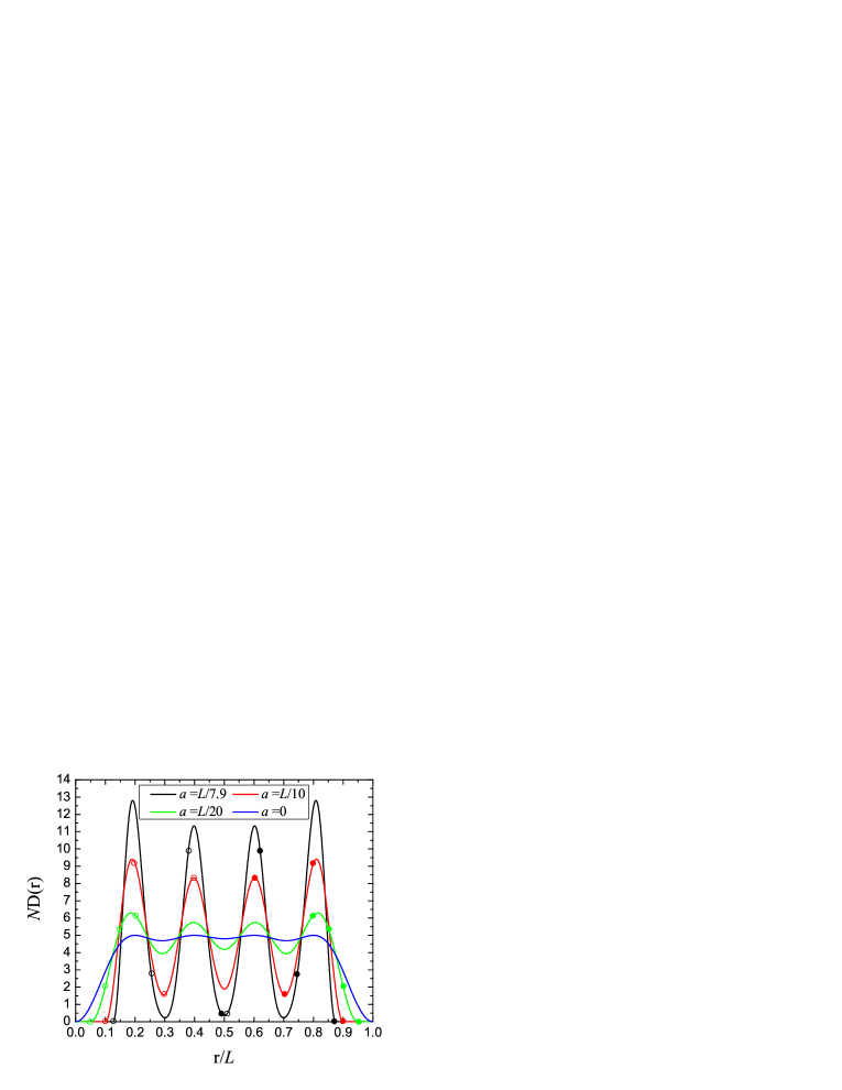
Figure 6: (color online) The pair distribution function $D(r)$ as a function of distance $r$ for $N=5$.

IV Bosons with $a>0$

For the one-dimensional hard sphere boson system, Girardeau Girardeau60 ; Girardeau65 has shown a Bose-Fermi mapping theorem which maps the hardcore boson system to a spinless hardcore fermion system, for $a>0$.

$$\Psi_{\text{BE}}(x_{1},x_{2},\cdots,x_{N})=|\Psi_{\text{FD}}(x_{1},x_{2},\cdots,x_{N})|.$$

The pair distribution function is related to the square of the wave function. Thus for $a>0$

$$D_{\text{BE}}(r)=D_{\text{FD}}(r).$$ (26)

References

(1)
L. Tonks, Phys. Rev. 50, 955 (1936).
(2)
E. Lieb and W. Liniger, Phys. Rev. 130, 1605 (1963).
(3)
E. Lieb, Phys. Rev. 130, 1616 (1963).
(4)
C. W. Ufford and E. P. Wigner, Phys. Rev. 61, 524 (1942).
(5)
M. Girardeau, J. Math. Phys. 1, 516 (1960).
(6)
M. D. Girardeau, Phys. Rev. 139, B500 (1965).
(7)
Y. Castin et al., J. Mod. Opt. 47, 2671 (2000).
(8)
D. M. Gangardt and G.V. Shlyapnikov, Phys. Rev. Lett. 90,
010401 (2003); New J. Phys. 5, 79 (2003).
(9)
K.V. Kheruntsyan et al., Phys. Rev. Lett. 91, 040403
(2003); Phys. Rev. A 71, 053615 (2005).
(10)
P. D. Drummond, P. Deuar, and K.V. Kheruntsyan, Phys. Rev. Lett.
92, 040405 (2004).
(11)
G. E. Astrakharchik and S. Giorgini, J. Phys. B 39, S1
(2006); M. Cazalilla, ibid. 37, S1 (2004); J.-S.
Caux and P. Calabrese, Phys. Rev. A 74, 031605(R) (2006).
(12)
A. Cherny and J. Brand, Phys. Rev. A 73, 023612 (2006).
(13)
A. G. Sykes et al., Phys. Rev. Lett. 100, 160406
(2008).
(14)
B. B. Wei and C. N. Yang, cond-mat/0807.2081 (2008).
(15)
C. N. Yang, Rev. Mod. Phys. 34, 694 (1962), §4.