Integrable theories and loop spaces: fundamentals, applications and new developments

Orlando Alvarez^a,, L. A. Ferreira^b, and J. Sánchez-Guillén^c,

^a Department of Physics
University of Miami
P.O. Box 248046
Coral Gables, FL 33124, USA

^b Instituto de Física de São Carlos; IFSC/USP;
Universidade de São Paulo
Caixa Postal 369, CEP 13560-970, São Carlos-SP, BRAZIL

^c Departamento de Fisica de Particulas, Universidad de Santiago
and Instituto Galego de Fisica de Altas Enerxias (IGFAE)
E-15782 Santiago de Compostela, SPAIN

We review our proposal to generalize the standard two-dimensional flatness construction of Lax-Zakharov-Shabat to relativistic field theories in $d+1$ dimensions. The fundamentals from the theory of connections on loop spaces are presented and clarified. These ideas are exposed using mathematical tools familiar to physicists. We exhibit recent and new results that relate the locality of the loop space curvature to the diffeomorphism invariance of the loop space holonomy. These result are used to show that the holonomy is abelian if the holonomy is diffeomorphism invariant.

These results justify in part and set the limitations of the local implementations of the approach which has been worked out in the last decade. We highlight very interesting applications like the construction and the solution of an integrable four dimensional field theory with Hopf solitons, and new integrability conditions which generalize BPS equations to systems such as Skyrme theories. Applications of these ideas leading to new constructions are implemented in theories that admit volume preserving diffeomorphisms of the target space as symmetries. Applications to physically relevant systems like Yang Mills theories are summarized. We also discuss other possibilities that have not yet been explored.

1 Introduction

Symmetry principles play a central role in Physics and other sciences. The laws governing the four fundamental interactions of Nature are based on two beautiful implementations of such ideas. The electromagnetic, weak and strong nuclear interactions have their basic structures encoded into the gauge principle that leads to the introduction of a non-integrable phase in the wave functions of the particles. The gravitational interaction originates from the principle of equivalence that leads to the general covariance of the dynamics under coordinate transformations.

An important and crucial issue in the success of these principles is the identification of the fundamental objects that are acted upon by the symmetry transformation. Those objects belong to a representation space of the transformation groups where dynamical consequences can be studied. Our understanding of the atomic, nuclear and particle phenomena has led us to a description of the world in terms of objects that have the dual character of point particles and waves. The symmetries we understand are formulated in terms of unitary representations on the Hilbert space of the quantum theory. The great lacuna in that formulation is Einstein’s Theory of General Relativity. We have not yet identified the quantum objects that could fully illuminate the symmetry principles of the gravitational interaction.

The other lacuna in our understanding of physical phenomena is the strong coupling regime or the non-perturbative regime of many theories. Even though this has apparently a more technical flavor it may hide some very important pieces of information in our quest for the description of Nature. The lack of non-perturbative methods has prevented or at most delayed developments in many fronts of our knowledge, from condensed matter physics to the confinement of quarks and gluons, weather prediction and a variety of mechanisms in biological systems. We may have the microscopic theories for practically all these phenomena but we just do not know how to solve them. There have been many successes in the strong coupling regime though the methods and the models are quite diverse. The discussions in this review are motivated by successes in certain low dimensional models that play an important role in many areas of Physics from condensed matter to high energy physics. We want to be concrete and to make clear the points that will be discussed in this review. Consider the simple and very well known sine-Gordon model. This is a $1+1$ dimensional field theory of a real scalar field $\phi$ with equation of motion

$$\partial_{t}^{2}\phi-\partial_{x}^{2}\phi+\frac{m^{2}}{\beta}\sin\left(\beta\,\phi\right)=0\,,$$ (1.1)

where $\beta$ is a dimensionless coupling constant and $m$ a mass parameter (in natural units where $c=\hbar=1$). The symmetries of this theory are the Poincaré group in two dimensions, and the discrete transformations $\phi\rightarrow\phi+\frac{2\,\pi\,n}{\beta}$, with $n$ an integer. Certainly these symmetries are important in the study of the model, but they are far from being responsible for the amazing properties this theory presents. In order to understand the full symmetry group of the model we have to describe the dynamics in terms of additional objects besides the scalar field $\phi$. You can easily verify that the sine-Gordon equation (1.1) is equivalent to a zero curvature condition

$$\partial_{+}\,A_{-}-\partial_{-}\,A_{+}+\left[\,{A_{+}}\,,\,{A_{-}}\,\right]=0$$ (1.2)

for a connection that is a functional of the scalar field $\phi$:

$$A_{+}=-\frac{m^{2}}{4}\left(\begin{array}[]{cc}0&e^{i\beta\,\phi}\\ \lambda\,e^{-i\beta\,\phi}&0\end{array}\right)\qquad\qquad A_{-}=\left(\begin{array}[]{cc}-\frac{i\beta}{2}\,\partial_{-}\phi&1/\lambda\\ 1&\frac{i\beta}{2}\,\partial_{-}\phi\end{array}\right).$$ (1.7)

Here we are using light cone coordinates $x_{\pm}=\left(x_{0}\pm x_{1}\right)/2$, and $A_{\pm}=A_{0}\pm A_{1}$, with $x_{0}$ and $x_{1}$ being the time and space coordinates respectively. The parameter $\lambda$ is arbitrary and may be chosen to be complex. It is called the spectral parameter and it makes the algebra, where the connection $A_{\mu}$ lives to be the infinite dimensional $sl(2)$ loop algebra. In terms of these new objects you can see that the sine-Gordon theory has an infinite dimensional group of symmetries given by the gauge transformations

$$A_{\mu}\rightarrow g\,A_{\mu}\,g^{-1}-\partial_{\mu}g\,g^{-1}$$ (1.8)

with $g$ being elements of the $sl(2)$ loop group ($\lambda$ dependent). These are called hidden symmetries because they are not symmetries of the equations of motion or of the Lagrangian. They play an important role in the development of exact methods in integrable field theories and practically all that is known in soliton theory is derived from the zero curvature condition (1.2). Exact solutions can be constructed using techniques like the inverse scattering or dressing methods. In addition, in $1+1$ dimensions, the flatness condition (1.2) is in fact a conservation law. One can show that the conserved quantities after the imposition of appropriate boundary conditions are given by the eigenvalues of the operator

$$W_{\Gamma}=P\exp\left[\int_{\Gamma}d\sigma\,A_{\mu}\,\frac{dx^{\mu}}{d\sigma}\right],$$ (1.9)

where $\Gamma$ is the spatial sub-manifold of space-time, and where $P$ means path ordering. By expanding in positive and negative powers of the spectral parameter $\lambda$ you get an infinite number of conserved charges. The evaluation of those charges can be better done by using the central extension of the loop algebra, the affine Kac-Moody algebra, using for instance the methods of [46].

For soliton theories belonging to the class of the sine-Gordon model, the so-called affine Toda theories, the hidden symmetries (1.8) can be understood in simpler terms. Such theories can be obtained by Hamiltonian reduction of the so-called two-loop WZNW model [19] that is invariant under the local symmetry group $G_{L}\times G_{R}$ where $G_{L/R}$ are two copies of the loop group mentioned above. By Hamiltonian reduction the corresponding Noether charges can be related to the conserved charges coming from the eigenvalues of the operator (1.9). The algebra of the reduced currents of the two-loop WZNW model is of the so-called $W$-algebra type and the associated symmetries seem to mix in a non-trivial way internal and space-time transformations.

The hidden symmetries associated to (1.8) are known to exist in theories defined on a two dimensional space-time. Of course the existence of similar structures in dimensions higher than two would be very important to understand the non-perturbative aspects of many physical phenomena. It is natural to ask if a change of the basic objects used to represent the dynamics of a theory could aid in investigating such structures. Some years ago we proposed an approach to construct what could perhaps be integrable theories in higher dimensions [18]. Since we are basically interested in finding symmetries beyond those already known in ordinary field theories, the main idea is to ponder how the conserved charges of the type (1.9) would look like in higher dimensions. We expect them to involve integrations on the spatial sub-manifold, and so in a $d+1$ dimensional space-time it would be an integration in $d$ dimensions. The conservation laws associated to (1.9) follow from the fact that the path ordered integrals of the connection $A_{\mu}$ are path independent, and that in turn follows, via the non-abelian Stokes theorem, from the flatness of the connection. So we need the generalization of the concept of a flat connection that can be integrated on a $d$ dimensional surface in space-time. As discussed in [18], the key concept is that of connections on loop spaces. Take the case of a $2+1$ dimensional space-time, where the relevant surface is two dimensional. We can fix a point $x_{0}$ on such surface and scan it with closed loops, starting and ending at $x_{0}$. The surface can therefore be seen as a collection of loops. By ordering the loops, the surface becomes therefore a path in the space of all loops. What we need therefore is a one-form connection on loop space. The path ordered integral of such connection on loop space will replace the operator (1.9) and its flatness condition leads to the conservation laws.

In order to implement such ideas we need to connect the objects in loop space with those in space-time. The proposal put forward in [18] was to construct a connection in loop space. For example, in the case of a $2+1$ dimensional space-time we suggested that a rank two antisymmetric tensor $B_{\mu\nu}$ and a one form connection $A_{\mu}$ were the necessary ingredients. The connection in loop space introduced in [18] was then

$${\cal A}\left(x^{\mu}\left(\sigma\right)\right)=\int_{\gamma}d\sigma\,W^{-1}\,B_{\mu\nu}\,W\,\frac{d\,x^{\mu}\left(\sigma\right)}{d\sigma}\,\delta x^{\nu}\left(\sigma\right)$$ (1.10)

where the integral is made on a loop $\gamma$ in space-time, parametrized by $\sigma$. The quantity $W$ is obtained from the connection $A_{\mu}$ through the differential equation

$$\frac{d\,W}{d\sigma}+A_{\mu}\,\frac{d\,x^{\mu}\left(\sigma\right)}{d\sigma}\,W=0$$ (1.11)

Notice that the quantity $W$ in (1.10) implements a parallel transport of $B_{\mu\nu}$, and that leads to better behaviour under gauge transformations. In order to obtain conservation laws we imposed the flatness condition on the connection on loop space

$$\delta{\cal A}+{\cal A}\wedge{\cal A}=0$$ (1.12)

For a space-time of dimension $d+1$ we had to consider generalized loop spaces, i.e., the space of maps from the sphere $S^{d-1}$ to the space-time. The connection will then be defined in terms of an antisymmetric tensor of rank $d$, and possibly additional lower rank tensors.

The purpose of the present paper is twofold. First we make a review of the proposal of [18] for the implementation of zero curvature conditions on loop spaces that lead to conservation laws and hidden symmetries for theories defined in a space-time of any dimension. We also review and discuss the developments that have followed from such approach giving many examples. Second we present new results about the method.

The most important new results are given in Section 2, and they are concerned with the concept of $r$-flatness. We have stated that the conserved charges are given by path ordered integrals of the connection in loop space. Such paths correspond to a surface in space-time. The charges should depend only the physical surface and not on the way we scan it with loops. In other words the charges should not depend upon the parametrization of the surface. Therefore, the path ordered integral of the connection on loop space should be re-parametrization invariant. A connection satisfying this is called $r$-flat. The most important result of section 2 is to show that a $r$-flat connection ${\cal A}$ in loop space must satisfy

$${\cal A}\wedge{\cal A}=0$$ (1.13)

Therefore, in order to have conservation laws we need the two summands in (1.12) to vanish separately. The second important result of Section 2 is that the holonomy group of $r$-flat connections in loop spaces is always abelian. These conditions drastically reduce the possible non-trivial structures we can have for the implementation of hidden symmetries for physical theories in a space-time of dimension higher than two. Our results have the character of a No-Go Theorem.

In Section 3 we discuss the local conditions in space-time which are sufficient for the vanishing of the curvature of the connection in loop space. Such local conditions are the ones that have been used in the literature to construct physical theories with an infinite number of conservation laws in any dimension. In Section 4 we provide some examples of such theories. The possibilities of using the approach for developing methods for the construction of exact solutions is discussed in Section 5 and many examples are given. Further applications of our approach to integrable theories in any dimension are given in Section 6 including some examples possibly relevant for the low energy limit (strong coupling) of gauge theories.

2 Connections in loop space

2.1 Philosophy

In this Section we discuss the theory of connections on loop spaces from a physicists viewpoint using geometrical and topological concepts at the level of the text by Nakahara [59]. Connections on loop spaces is an old subject in the physics literature, see for example [54, 60]. We restrict our discussion in this Section to what is needed in applications to integrable models. We present the ideas developed in [18] and new results in a slightly different way that is faithful to the original presentation. The motivation for that work was the generalization to higher dimensions of the ideas and of the technology that was developed around the Lax-Zakharov-Shabat framework[56] for integrable systems in $(1+1)$-dimensions. The basic idea is that the equations of motion may be formulated as a flatness condition with an appropriate connection. The holonomy of the connection is independent of the loop used and the holonomy can be massaged to construct an infinite number of conservation laws. The $(1+1)$ conservation laws involve traces of the holonomy, $\operatorname{Tr}\exp\left(\int A\right)$, using an ordinary connection. The generalization to a $(2+1)$-dimensional spacetime should be an object of the type $\operatorname{Tr}\exp\left(\int B\right)$ where $B$ is now a $2$-form since space is two dimensional. Continuing in this fashion you would require an $n$-form $B^{(n)}$ in the $(n+1)$-dimensional case where the answer would be $\operatorname{Tr}\exp\left(\int B^{(n)}\right)$.

What is the meaning of these integrals when the $B^{(n)}$ take values in a non-abelian Lie algebra? Our approach was to indirectly address this question by writing down a differential equation whose solution would be the desired integral. This is analogous to using the parallel transport equation, a differential equation for the Wilson line, as way of defining $\exp\left(\int A\right)$. In fact we well know that if $A$ is non-abelian $\exp\left(\int A\right)$ is not the correct expression. The solution to the differential equation is a path ordered exponential. We wanted to use the same philosophy in higher dimension and let the differential equation tell us what is supposed to replace $\exp\left(\int B^{(n)}\right)$. To get conservation laws in higher dimensions we needed an analog of the flatness condition on the connection $A$ and an analog of holonomy. The idea is to use the differential equation to define the holonomy. Requiring that the holonomy be independent of the submanifold led to “zero curvature” conditions that were local and non-local.

The original framework we developed for an $(n+1)$-dimensional spacetime led to an inductive solution. First we solved the problem for a $1$-form $A$. Second, introduce a $2$-form $B$ and use $A$ and the already solved problem to solve the problem on a $2$-manifold. Third, introduce a $3$-form $B^{(3)}$ and use the already solved $2$-dimensional problem to solve the new $3$-manifold problem. This procedure continues all the way to an $n$-form $B^{(n)}$. In this way we defined a holonomy associated with the $n$-manifold. Requiring that the holonomy be invariant with respect to deformations of this manifold led to local and non-local “zero curvature” conditions.

The procedure just described had a very unsatisfactory aspect. First what we are doing is constructing a submanifold. We start with a point and move it to construct a curve. The curve is developed in $1$-dimension to get a surface. This surface is then developed into a $3$-manifold, etc., until we get a $n$-manifold. Our differential equations are integrated precisely in the order of this construction. This means that the holonomy will in general depend on the parametrization used to develop the manifold. If we perform a diffeomorphism on this manifold, i.e., a reparametrization and effectively a redevelopment, then we do not expect to get the same holonomy. This was not a problem for us because the “zero curvature” conditions we needed to study integrable systems solved the problem. Still, the procedure is very unsatisfactory and we searched for a better formulation. Additionally, there was a great simplification. In many models we considered and from the general form of the field equations, we noted that the $1$-form $A$ and the $n$-form $B^{(n)}$ sufficed.

The framework of the inductive procedure strongly suggested that we had connections on some appropriate path space. As soon as we restricted to a $1$-form $A$ and $n$-form $B^{(n)}$ it became clear how to write down a connection like object on an appropriate loop space and to show that the change in holonomy when deforming a path in the loop space gave the curvature of the connection. Flatness of the curvature led to a holonomy that did not change if the manifold was deformed. Also, the holonomy was automatically invariant under the action of the diffeomorphism group of the manifold for “zero curvature” connection thus restoring “relativistic invariance”.

There is a large mathematical body of literature devoted to developing a theory of non-abelian connections on loop spaces. It is not clear whether this is the correct approach for a theory of connections on loop spaces. The mathematical concepts used in these approaches are much more sophisticated than what we require to discuss applications of connections on higher loop spaces to integrable models. The subject is very Category Theory oriented and beyond the charge of this review. Explaining concepts such as abelian gerbes, non-abelian gerbes, abelian gerbes with connection, non-abelian gerbes with connection, $2$-groups, $2$-bundles, $2$-connections, etc., would be a long review article in itself. Here we provide a selection of papers that are relevant to our applications and provide contemporary viewpoints on the subject [22, 23, 53, 26, 66, 27, 28, 31, 67].

In summary, connections on loop spaces provides a suitable but not totally satisfying generalization of the Lax-Zakharov-Shabat scenario. The current framework suffers from non-locality and does not appear to have enough structure to give a satisfactory construction of conservation laws. It is our belief that the current theory of connections on loop spaces is not quite correct because there are too many non-localities even at step one. We do not know what the final set up will be but we do know that the current set up is good enough for some applications.

2.2 Curvature and holonomy

Locality plays a very important role in physics and for this reason we require all our constructions to use local data. We have a spacetime manifold $M$ where all the action takes place. For simplicity we always assume that $M$ is connected and simply connected. For example in the Lax-Zakharov-Shabat case $M$ may be taken to be a $(1+1)$ dimensional lorentzian cylinder. In a higher dimensional example $M$ may be $\mathbb{R}\times S^{d}$.

For future reference we note that if $\alpha$ and $\beta$ are $1$-forms and if $u$ and $v$ are vector fields then $(\alpha\wedge\beta)(u,v)=\alpha(u)\beta(v)-\alpha(v)\beta(u)$. We use the standard physics notation for the Heaviside step function:

$$\theta(x)=\begin{cases}1,&x>0\,,\\ 0,&x<0\,.\end{cases}$$

The geometric data we manipulate comes from a principal bundle [59, 55]. Assume you have a manifold $X$ and a principal fiber bundle $\pi:P\to X$ with connection $A$ and curvature $F$. The structure group $G$ of the principal bundle is a connected finite dimensional Lie group with Lie algebra $\mathfrak{g}$. The fiber over $x\in X$ will be denoted by $P_{x}$. Locally, a connection $A$ is a $\mathfrak{g}$-valued $1$-form on the manifold $X$.

For $x_{0}\in X$, let $\Omega(X,x_{0})$ be the space of parametrized loops with basepoint $x_{0}$. We view a loop in $\gamma\in\Omega(X,x_{0})$ as a map $x:S^{1}\to X$ with a basepoint condition. To make this more explicit, the circle $S^{1}$ is parametrized by the interval $[0,2\pi]$. The basepoint condition on the map $x$ is $x(2\pi)=x(0)=x_{0}$. The space of all loops will be denoted by $\displaystyle\mathcal{L}(X)=\cup_{x\in X}\Omega(X,x)$.

Let $\gamma\in\Omega(X,x_{0})$ and let $W$ be parallel transport (Wilson line) along $\gamma$ associated with the connection $A$. We solve the parallel transport equation

$$\frac{d}{d\tau}W(\tau)+A_{\mu}(x(\tau))\,\frac{dx^{\mu}}{d\tau}\;W(\tau)=0\,,$$ (2.1)

along the loop $\gamma$ with initial condition $W(0)=I$. Let $f:[0,2\pi]\to[0,2\pi]$ be a diffeomorphism of the interval that leaves the endpoints fixed, i.e., $f(0)=0$ and $f(2\pi)=2\pi$. If $\tilde{\tau}=f(\tau)$ is a new parametrization of the interval then the holonomy is independent of the parametrization. This is easily seen by inspecting (2.1). You can generalize this to allow for back tracking. Any two loops that differ by backtracking give the same holonomy. The holonomy depends only on the point set of the loop and not on the parametrization of the loop.

Consider a deformation of $\gamma$ prescribed by a vector field $\bm{N}$. The change in holonomy, see [18, eq. (2.7)], is given by

$$W^{-1}(2\pi)\bigl{(}\delta W(2\pi)\bigr{)}=\int_{0}^{2\pi}d\tau\;W^{-1}(\tau)F\bigl{(}\bm{T}(\tau),\bm{N}(\tau)\bigr{)}W(\tau)\,,$$ (2.2)

where $\bm{T}$ is the tangent vector to the curve $\gamma$. This variational formula requires the basepoint to be kept fixed otherwise there is an additional term. We obtain the standard result that the holonomy does not vary under a homotopy (continuous deformation) if and only if the curvature vanishes.

It is also worthwhile to connect (2.2) to the holonomy theorem of Ambrose and Singer [55]. The intuition developed here is useful in understanding some of the ideas we will pursue in loop spaces. Pick a basepoint $x_{0}$ on a finite dimensional manifold $X$. Let $\gamma\in\Omega(M,x_{0})$ be a contractible loop. Parallel transport around $\gamma$ gives a group element $W(2\pi)=W(\gamma)$ called the holonomy of $\gamma$. The set $\{W(\gamma)\}$ for all contractible $\gamma\in\Omega(M,x_{0})$ is a subgroup of $G$ called the restricted holonomy group and denoted by $H_{x_{0}}$. A result of the Ambrose-Singer theorem is that the Lie algebra of $H_{x_{0}}$ is related to the curvature $F$ of the connection in a way we now make more precise.

Figure 1: The top figure schematically represents a loop based at $x_{0}$ where you go out to a point $x$ and return along the same curve. In the bottom figure you go to $x$ and then go around a small “infinitesimal circle” and return along the initial curve. A mathematician’s lasso is a loop that looks like the bottom figure. We are interested in comparing the holonomies between the top and the bottom loops.

Consider a point $x\in X$ and a path $p$ from $x_{0}$ to $x$. On every tangent $2$-plane at $x$ evaluate the curvature and parallel transport that to $x_{0}$ along $p$ giving you Lie algebra elements in $\mathfrak{g}$. Consider the collection of all such elements as you consider all all paths connecting $x_{0}$ to $x$ and all $x\in X$. The set of all these elements spans a vector subspace $\mathfrak{h}\subset\mathfrak{g}$. A consequence of the Ambrose-Singer theorem is that $\mathfrak{h}$ is the Lie algebra of the restricted holonomy group $H_{x_{0}}$. In Figure 1 we have two loops. The bottom loop is a small deformation of the top one. The holonomy for the top loop is $W(2\pi)=I$. The difference between the holonomies of the top and bottom loops may be computed using (2.2). We see that $\delta W(2\pi)$ only gets a contribution from the small infinitesimal circle. This contribution is the curvature of the $2$-plane determined by the deformation of the loop. That curvature is subsequently parallel transported back to $x_{0}$ and gives us the Lie algebra element $\delta W(2\pi)$.

Remark 2.1.

Observe that $\varpi:\mathcal{L}(X)\to X$ is a fiber bundle with projection given by the starting point map $\varpi(\gamma)=\gamma(0)$ where $\gamma:[0,2\pi]\to X$ is a loop. The fiber over $x\in X$ is $\Omega(X,x)$. We can use the map $\varpi:\mathcal{L}(X)\to X$ to pullback the principal bundle $\pi:P\to X$ to a principal bundle $\tilde{\pi}:\widetilde{P}\to\mathcal{L}(X)$. The fiber over $\gamma\in\mathcal{L}(X)$ is isomorphic to $P_{\gamma(0)}$. The structure group is still the finite dimensional group $G$.

Remark 2.2.

Next we notice that equation (2.2) is valid even if the manifold $X$ is itself a loop space. To see how this works assume we have a finite dimensional target space $M$ and we consider a loop in $M$ that we are going to deform. Usually we look at a finite $r$ parameter deformation. So we have a family of loops that we parametrize as $x(\sigma;q^{1},q^{2},\ldots,q^{r})$ where $\sigma$ is the loop parameter. We can view this as a map $\phi:Q\to\mathcal{L}(M)$ where $Q$ is an $r$-dimensional manifold. We use $\phi$ to pullback the bundle $\widetilde{P}$ back to $Q$ and we are in a finite dimensional situation where we know that (2.2) is valid.

2.3 Connections on loop space

Now we specialize to the first case of interest where $X=\mathcal{L}(M)$ for some finite dimensional target space $M$. For technical reasons related to the behavior of the holonomy when you vary the endpoints of a path it is convenient to fix the basepoint of the loops and this is the explanation of why we restrict ourselves to $\Omega(M,x_{0})\hookrightarrow\mathcal{L}(M)$. We have a principal fiber bundle $\tilde{\pi}:\widetilde{P}\to\mathcal{L}(M)$ with fiber isomorphic to $P_{\gamma(0)}$ that we can restrict to $\Omega(M,x_{0})$. This is the bundle we will be using and we will also call it $\widetilde{P}$. Let $B=\tfrac{1}{2}B_{\mu\nu}(x)dx^{\mu}\wedge dx^{\nu}$ be a $\mathfrak{g}$-valued $2$-form on $M$ that transforms via the adjoint representation under gauge transformation of $P$. Let $\delta$ be the exterior derivative on the space $\Omega(M,x_{0})$, we know that $\delta^{2}=0$ and

$$\delta x^{\mu}(\sigma)\wedge\delta x^{\nu}(\sigma^{\prime})=-\delta x^{\nu}(\sigma^{\prime})\wedge\delta x^{\mu}(\sigma)\;.$$

Here $\sigma\in[0,2\pi]$ is the parameter along the loop. Because the basepoint $x_{0}$ is fixed we must have $\delta x^{\mu}(0)=\delta x^{\mu}(2\pi)=0$. We use $A$ and $B$ to construct [18] a connection $\mathcal{A}$ on $\tilde{\pi}:\widetilde{P}\to\Omega(M,x_{0})$ by

$$\mathcal{A}[\gamma]=\int_{0}^{2\pi}d\sigma\;W(\sigma)^{-1}B_{\mu\nu}(x(\sigma))W(\sigma)\frac{dx^{\mu}}{d\sigma}\delta x^{\nu}(\sigma)\,.$$ (2.3)

In the above, the loop $\gamma\in\Omega(M,x_{0})$ is described by the map $x:[0,2\pi]\to M$, the parallel transport (Wilson line) $W(\sigma)$ is along $\gamma$ from $x(0)=x_{0}$ to $x(\sigma)$ using the connection $A$ on $P$. Note that at each $\sigma$,

$$B_{\mu\nu}(x(\sigma))\frac{dx^{\mu}}{d\sigma}\delta x^{\nu}(\sigma)$$

is a $\mathfrak{g}$-valued $1$-form at $x(\sigma)$ that is parallel transported back using $W(\sigma)$ to $x(0)$ where all the parallel transported objects are added together at the common endpoint. Parallel transport gives an identification of the different fibers of $P\to M$ and this is used to add together the various Lie algebra elements in (2.3). Note the the connection $\mathcal{A}$ is a $\mathfrak{g}$-valued $1$-form on $\Omega(M,x_{0})$. The Lie algebra element is associated with the fiber $P_{\gamma(0)}\approx G$.

Morally, our definition of $\mathcal{A}$ is motivated by the following canonical construction. Let $\operatorname{ev}:S^{1}\times\Omega(M,x_{0})\to M$ be the evaluation map defined by $\operatorname{ev}:(\sigma,\gamma)\mapsto\gamma(\sigma)$. Given a $2$-form $B$ on $M$ you can construct a $1$-form $\mathcal{A}$ on $\Omega(M,x_{0})$ via pullback and integration. The pullback $\operatorname{ev}^{*}B$ is a $2$-form on $S^{1}\times\Omega(M,x_{0})$ and therefore integrating over the circle

$$\int_{S^{1}}\operatorname{ev}^{*}B$$

reduces the degree by one and gives a $1$-form on $\Omega(M,x_{0})$.

The connection defined by (2.3) is reparametrization (diffeomorphism) invariant. To show this choose a diffeomorphism $g:[0,2\pi]\to[0,2\pi]$ that leaves the endpoints fixed and let $\tilde{\gamma}$ be the parametrized loop given by the map $\tilde{x}=x\circ g$. The it is easy to see that $\mathcal{A}[\tilde{\gamma}]=\mathcal{A}[\gamma]$. For future reference, the new parametrization of the loop will be denoted by $\tilde{\sigma}=g(\sigma)$.

The following notational convention is very useful. For any object $X$ which transforms under the adjoint representation, parallel transport it from $x(\sigma)$ to $x(0)$ along $\gamma$ and denote this parallel transported object by

$$X^{W}(\sigma)=W(\sigma)^{-1}X(x(\sigma))W(\sigma)\;.$$ (2.4)

An elementary exercise shows that

$$\frac{d}{d\sigma}X^{W}=W(\sigma)^{-1}(D_{\mu}X)\bigl{(}x(\sigma)\bigr{)}W(\sigma)\;\frac{dx^{\mu}}{d\sigma}\;.$$ (2.5)

The curvature $\mathcal{F}=\delta\mathcal{A}+\mathcal{A}\wedge\mathcal{A}$ is given by, see [18, Sec. 5.3],

$$\mathcal{F} =-\frac{1}{2}\int_{0}^{2\pi}d\sigma\;W(\sigma)^{-1}\left[D_{\lambda}B_{\mu\nu}+D_{\mu}B_{\nu\lambda}+D_{\nu}B_{\lambda\mu}\right](x(\sigma))W(\sigma)$$

$$\mathstrut\hskip 36.135pt\times\frac{dx^{\lambda}}{d\sigma}\delta x^{\mu}(\sigma)\wedge\delta x^{\nu}(\sigma)$$

$$\quad-\int_{0}^{2\pi}d\sigma\int_{0}^{\sigma}d\sigma^{\prime}\;\left[F^{W}_{\kappa\mu}(x(\sigma^{\prime})),B^{W}_{\lambda\nu}(x(\sigma))\right]\frac{dx^{\kappa}}{d\sigma^{\prime}}\frac{dx^{\lambda}}{d\sigma}\delta x^{\mu}(\sigma^{\prime})\wedge\delta x^{\nu}(\sigma)$$

$$\quad+\frac{1}{2}\int_{0}^{2\pi}d\sigma\int_{0}^{2\pi}d\sigma^{\prime}\left[B^{W}_{\kappa\mu}(x(\sigma^{\prime})),B^{W}_{\lambda\nu}(x(\sigma))\right]\frac{dx^{\kappa}}{d\sigma^{\prime}}\frac{dx^{\lambda}}{d\sigma}\delta x^{\mu}(\sigma^{\prime})\wedge\delta x^{\nu}(\sigma)\;.$$ (2.6)

The last summand above may be rewritten as

$$\int_{0}^{2\pi}d\sigma\int_{0}^{\sigma}d\sigma^{\prime}\left[B^{W}_{\kappa\mu}(x(\sigma^{\prime})),B^{W}_{\lambda\nu}(x(\sigma))\right]\frac{dx^{\kappa}}{d\sigma^{\prime}}\frac{dx^{\lambda}}{d\sigma}\delta x^{\mu}(\sigma^{\prime})\wedge\delta x^{\nu}(\sigma)$$

by observing that the integrand is symmetric under the interchange of $\sigma$ and $\sigma^{\prime}$. You have to take into account both the anti-symmetry of the Lie bracket and the anti-symmetry of the wedge product. This means that (2.6) takes the form

$$\mathcal{F} =-\frac{1}{2}\int_{0}^{2\pi}d\sigma\;W(\sigma)^{-1}\left[D_{\lambda}B_{\mu\nu}+D_{\mu}B_{\nu\lambda}+D_{\nu}B_{\lambda\mu}\right](x(\sigma))W(\sigma)$$

$$\qquad\qquad\times\frac{dx^{\lambda}}{d\sigma}\;\delta x^{\mu}(\sigma)\wedge\delta x^{\nu}(\sigma)$$

$$\quad+\int_{0}^{2\pi}d\sigma\int_{0}^{\sigma}d\sigma^{\prime}$$

$$\qquad\times\left[B^{W}_{\kappa\mu}(x(\sigma^{\prime}))-F^{W}_{\kappa\mu}(x(\sigma^{\prime})),B^{W}_{\lambda\nu}(x(\sigma))\right]\frac{dx^{\kappa}}{d\sigma^{\prime}}\frac{dx^{\lambda}}{d\sigma}\;\delta x^{\mu}(\sigma^{\prime})\wedge\delta x^{\nu}(\sigma)\,.$$

We write the components of the curvature $2$-form $\mathcal{F}$ in a more skew symmetric way

$$\mathcal{F} =-\frac{1}{2}\int_{0}^{2\pi}d\sigma\;W(\sigma)^{-1}\left[D_{\lambda}B_{\mu\nu}+D_{\mu}B_{\nu\lambda}+D_{\nu}B_{\lambda\mu}\right](x(\sigma))W(\sigma)$$

$$\qquad\qquad\times\frac{dx^{\lambda}}{d\sigma}\;\delta x^{\mu}(\sigma)\wedge\delta x^{\nu}(\sigma)$$ (2.7a)

$$\quad+\frac{1}{2}\int_{0}^{2\pi}d\sigma\int_{0}^{2\pi}d\sigma^{\prime}\biggl{(}\theta(\sigma-\sigma^{\prime})\left[B^{W}_{\kappa\mu}(x(\sigma^{\prime}))-F^{W}_{\kappa\mu}(x(\sigma^{\prime})),B^{W}_{\lambda\nu}(x(\sigma))\right]$$

$$\qquad-\theta(\sigma^{\prime}-\sigma)\left[B^{W}_{\lambda\nu}(x(\sigma))-F^{W}_{\lambda\nu}(x(\sigma)),B^{W}_{\kappa\mu}(x(\sigma^{\prime}))\right]\biggr{)}$$

$$\qquad\times\frac{dx^{\kappa}}{d\sigma^{\prime}}\frac{dx^{\lambda}}{d\sigma}\;\delta x^{\mu}(\sigma^{\prime})\wedge\delta x^{\nu}(\sigma)\,.$$ (2.7b)

This curvature contains two parts. There is a term that is local in $\sigma$ and involves the exterior covariant differential of $B$ which is the three form $D_{A}B$. There is a term that is non-local in $\sigma$ and involves Lie brackets of $B$ and $F$. If you want the physics to be local this term is a bit disturbing and we will discuss it presently.

There are two basic examples of a flat connection. There is a simple lemma that follows from (2.7) and the Bianchi identity $D_{A}F=0$.

Lemma 2.1.

If $B=F$ then $\mathcal{F}=0$, i.e., $\mathcal{A}$ is flat.

This case was studied in [31, 66]. Presently there are no known applications of $B=F$ to integrability. The other example is the case we discussed in our studies of integrability [18].

Lemma 2.2.

If $A$ is a flat connection on $P$, if the values of $B$ belong to an abelian ideal $\mathfrak{p}$ of $\mathfrak{g}$, and $D_{A}B=0$ then $\mathcal{F}=0$, i.e., $\mathcal{A}$ is flat.

First we note that saying that $B$ takes values in an ideal (not necessarily abelian) is a gauge invariant statement. A subalgebra is generally not invariant under group conjugation and therefore not compatible with a gauge invariant characterization. Note that if $M$ is connected and simply connected then we can use the flat connection to globally trivialize the principal bundle $P$ and we can be very explicit about what it means to say the $B$ has values in an abelian ideal. Namely pick a reference point in $M$ and parallel transport the abelian ideal $\mathfrak{p}$ to all other points in $M$. The flatness of $A$ and $\pi_{1}(M)=0$ tells us that this identification is independent of the path chosen for parallel transport. For us, these conditions were sufficient to construct an infinite number of conserved charges using holonomy in analogy to integrable models in $(1+1)$-dimensions.

We can apply (2.2) to extend the standard result relating holonomy and curvature to the loop space case. To compute the holonomy we need a loop in the loop space $\Omega(M,x_{0})$ with “basepoint” $\gamma_{0}\in\Omega(M,x_{0})$. A loop in $\Omega(M,x_{0})$ is given by a map $x:[0,2\pi]^{2}\to M$. If we use coordinates $(\sigma,\tau)$ on $[0,2\pi]^{2}$ then our map satisfies the boundary conditions $x(\sigma,0)=x(\sigma,2\pi)=\gamma_{0}(\sigma)$ and $x(0,\tau)=x(2\pi,\tau)=x_{0}$. For fixed $\tau$ the map $x_{\tau}(\sigma):[0,2\pi]\to M$ given by $x_{\tau}(\sigma)=x(\sigma,\tau)$ is a loop in $M$, i.e., $x_{\tau}\in\Omega(M,x_{0})$. The parameter $\tau$ gives the “time” development of the loop. We compute the holonomy using (2.1) with connection (2.3). Let $\Gamma$ denote the parametrized loop of loops given by the map $x:[0,2\pi]^{2}\to M$. $\Gamma$ is the image of a torus, see Figure 2.

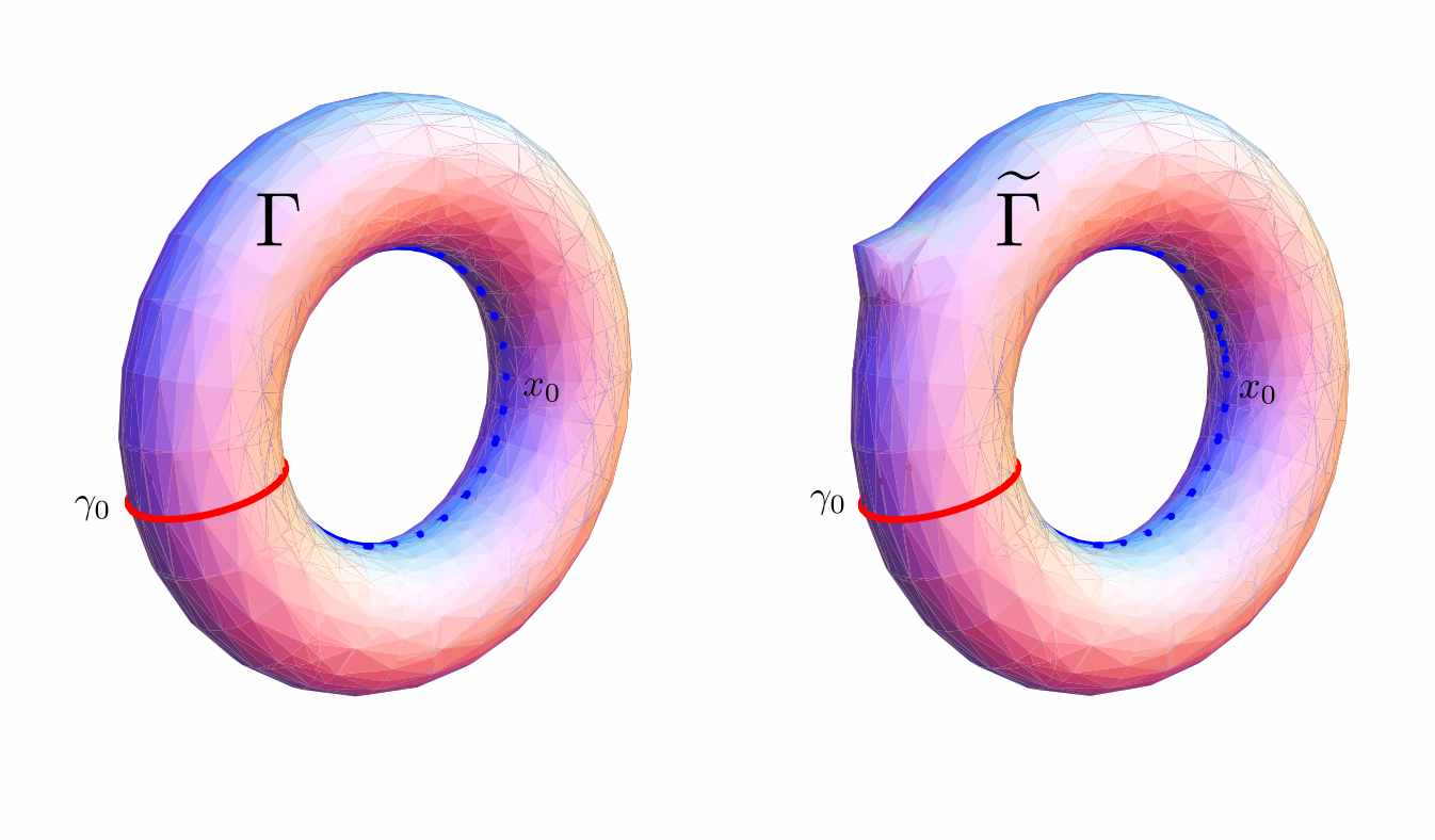
Figure 2: On the left is the loop of loops $\Gamma$. This is a torus with “basepoint” $\gamma_{0}$. The dotted vertical circle is mapped to $x_{0}$. On the right we have $\widetilde{\Gamma}$, a localized deformation of $\Gamma$. We are interested in comparing the difference in holonomy between the two. You should shrink the vertical interior circle (representing $x_{0}$) to a point and think of the above as doughnuts with very small holes.

Let $\operatorname{hol}(\Gamma)$ be the holonomy of $\Gamma$ computed by integrating the differential equation using the loop connection $\mathcal{A}$. If the torus $\Gamma$ is infinitesimally deformed while preserving the boundary conditions then $\delta(\operatorname{hol}(\Gamma))=0$ for all deformations if and only if $\mathcal{F}=0$. This is a consequence of applying Remark 2.2 and equation (2.2) to $\Gamma$ and its deformations.

2.4 Holonomy and reparametrizations

There is a drawback with this framework and that is that the holonomy depends on the parametrization of $\Gamma$. To understand this we go through the mechanics of the computation. Fix $\tau$ and use $x_{\tau}(\sigma)$ to compute the connection $\mathcal{A}[x_{\tau}]$. In doing this computation we have to compute the Wilson line $W$ (with connection $A$) that clearly depends on the loops $\{x_{\tau}\}$. Next we integrate differential equation (2.2) to get the $\tau$ development of parallel transport for connection $\mathcal{A}$. It is clear from this discussion that $\sigma$ and $\tau$ play very different roles and there is a prescribed order of integrating in the $\sigma$ and $\tau$ directions. We expect the holonomy to be different under two distinct parametrizations $(\sigma,\tau)$ and $(\tilde{\sigma},\tilde{\tau})$ as discussed in Figure 3.

Figure 3: On the left is parametrization by $(\sigma,\tau)$. The constant $\tau$ segments that determine $x_{\tau}$ are the dotted segments on the left and these are used to compute the connection $\mathcal{A}[x_{\tau}]$. A diffeomorphism of the square (that leaves the boundary fixed) leads to a new parametrization $(\tilde{\sigma},\tilde{\tau})$ where the horizontal segments from the left become the wavy curves on the right. To compute $\mathcal{A}[\tilde{x}_{\tilde{\tau}}]$ we need horizontal $\tilde{\tau}$ constant segments so we are going to get very different results.

A diffeomorphism $h:[0,2\pi]^{2}\to[0,2\pi]^{2}$ of the square gives a new parametrization $(\tilde{\sigma},\tilde{\tau})=h(\sigma,\tau)$ and a new torus $\widetilde{\Gamma}$. The images $\Gamma$ and $\widetilde{\Gamma}$ are the same point set in $M$. We assume for expositional simplicity that this point set is a smooth $2$-dimensional submanifold of $M$. As just discussed we expect that $\operatorname{hol}(\Gamma)\neq\operatorname{hol}(\widetilde{\Gamma})$ in general. There are three basic examples where the holonomy will be the same. If the diffeomorphism is of the form $(\tilde{\sigma},\tilde{\tau})=(g(\sigma),\tau)$ then the connection $\mathcal{A}$ does not change and you get the same result. If the diffeomorphism is of the form $(\tilde{\sigma},\tilde{\tau})=(\sigma,f(\tau))$ then the discussion following (2.1) applies. A function composition of these two cases where you have a diffeomorphism of the form $(\tilde{\sigma},\tilde{\tau})=(g(\sigma),f(\tau))$ also leaves the holonomy fixed.

Many of the models of interest of us are local field theories that can be made diffeomorphism invariant and for this reason we would like to try to understand the conditions that lead to a reparametrization invariant holonomy. We would like the holonomy to be geometrical and only depend on the image of the map $x(\sigma,\tau)$ and not on the details of the parametrization. If $\operatorname{hol}(\Gamma)=\operatorname{hol}(\widetilde{\Gamma})$ for all diffeomorphisms of $[0,2\pi]^{2}$ then we say that the connection $\mathcal{A}$ is r-flat (reparametrization flat) A consequence of the definition of $r$-flatness and of the holonomy deformation equation (2.2) is that a flat connection $\mathcal{A}$ is automatically $r$-flat.

Lemma 2.3.

A flat $\mathcal{A}$ connection is $r$-flat.

We work out the condition for $r$-flatness for infinitesimal diffeomorphisms. We look at the holonomy of our torus $\Gamma$. What distinguishes flatness from $r$-flatness is that in the former case the holonomy is not changed by an arbitrary deformation $\delta x^{\mu}$ while in the latter case the deformation has to be tangential to the $2$-manifold $\Gamma$. The tangent vector $\bm{T}$ to the loop $x_{\tau}$ is given by

$$\bm{T}=\frac{\partial x^{\mu}}{\partial\tau}\;\frac{\partial}{\partial x^{\mu}}\,.$$ (2.8)

The “spatial tangent vector” along the loop $x_{\tau}$ is

$$\bm{S}=\frac{\partial x^{\mu}}{\partial\sigma}\;\frac{\partial}{\partial x^{\mu}}\,.$$ (2.9)

Finally, a general deformation tangential to the $2$-submanifold $\Gamma$ is given by

$$\bm{N}=a(\sigma,\tau)\bm{S}+b(\sigma,\tau)\bm{T}\,,$$ (2.10)

where $a$ and $b$ are arbitrary functions vanishing on the boundary of the square $[0,2\pi]^{2}$. The condition for $r$-flatness will be given by inserting $\bm{T}$ and $\bm{N}$ into (2.2) and requiring the change in holonomy to vanish. We remark that $r$-flatness is automatic by construction in the $1$-dimensional case. It becomes a new non-trivial phenomenon in the $2$-dimensional case. It is really a statement about holonomy that we try to capture in terms of information contained in the curvature.

Theorem 2.4.

The connection $\mathcal{A}$ is $r$-flat if and only if for all maps $x:[0,2\pi]^{2}\to M$ we have

$$0 =\int_{0}^{2\pi}d\sigma^{\prime}\;\biggl{(}\theta(\sigma-\sigma^{\prime})\left[\left\{F^{W}_{\kappa\mu}(x(\sigma^{\prime},\tau^{\prime}))-B^{W}_{\kappa\mu}(x(\sigma^{\prime},\tau^{\prime}))\right\},B^{W}_{\lambda\nu}(x(\sigma,\tau))\right]$$

$$\qquad\qquad-\theta(\sigma^{\prime}-\sigma)\left[\left\{F^{W}_{\lambda\nu}(x(\sigma,\tau))-B^{W}_{\lambda\nu}(x(\sigma,\tau))\right\},B^{W}_{\kappa\mu}(x(\sigma^{\prime},\tau^{\prime}))\right]\biggr{)}$$

$$\qquad\times\frac{\partial x^{\kappa}}{\partial\sigma^{\prime}}\frac{\partial x^{\mu}}{\partial\tau^{\prime}}\frac{\partial x^{\lambda}}{\partial\sigma}\frac{\partial x^{\nu}}{\partial\tau}\quad\text{for $\tau=\tau^{\prime}$}.$$ (2.11)

Note that all the action occurs at “equal time”. A key observation required in proving this theorem is that the tangent space to the $2$-manifold is two dimensional and spanned by $\bm{S}$ and $\bm{T}$. This and the fact that in (2.7a) everything is at the same value of $\sigma$ means that $D_{A}B(\bm{S},\bm{T},\bm{N})=0$ automatically because $D_{A}B$ is a $3$-form. Therefore we will only get a contribution from the nonlocal (2.7b) term. Even here things simplify because there is no contribution from the $\bm{S}$ summand in (2.10) because there is always a contraction of two $\bm{S}$ vectors at the same $(\sigma,\tau)$ with some $2$-form. We only have to worry about the $\bm{T}$ summand in (2.10). A straightforward computation gives the equation above.

Corollary 2.5.

If $F=0$ and $B$ takes values in an abelian ideal $\mathfrak{p}$ of $\mathfrak{g}$ then the connection $\mathcal{A}$ is $r$-flat.

Using (2.4) we see that something that takes values in the ideal $\mathfrak{p}$ will remain in $\mathfrak{p}$ under parallel transport. Notice that we do not have to impose $DB=0$ to obtain $r$-flatness. Connections of this type are examples of $r$-flat connections that are not flat, i.e., $\mathcal{F}\neq 0$. The curvature $\mathcal{F}$ which is locally given by $D_{A}B$ will take values in $\mathfrak{p}$. There are examples of such connections. In reference [18] we constructed some models based on a non-semisimple Lie algebra $\mathfrak{g}$ that contains a non-trivial abelian ideal $\mathfrak{p}$. These models are automatically $r$-flat without imposing $DB=0$ which was necessary for our integrability studies.

The case $F=B$ leads automatically to a $r$-flat connection by Lemma 2.3. The converse is also true.

Corollary 2.6.

An $r$-flat connection $\mathcal{A}$ satisfying $B=F$ is also flat.

The proof is elementary because the Bianchi identity $D_{A}F=0$ automatically implies that $D_{A}B=0$. We remind the reader of Lemma 2.1

A connection $\mathcal{A}$ is said to be curvature local if the nonlocal commutator term in (2.7) for $\mathcal{F}$ vanishes. In other words, we have

$$0 =\biggl{(}\theta(\sigma-\sigma^{\prime})\left[B^{W}_{\kappa\mu}(x(\sigma^{\prime}))-F^{W}_{\kappa\mu}(x(\sigma^{\prime})),B^{W}_{\lambda\nu}(x(\sigma))\right]$$

$$\qquad-\theta(\sigma^{\prime}-\sigma)\left[B^{W}_{\lambda\nu}(x(\sigma))-F^{W}_{\lambda\nu}(x(\sigma)),B^{W}_{\kappa\mu}(x(\sigma^{\prime}))\right]\biggr{)}\frac{dx^{\kappa}}{d\sigma^{\prime}}\frac{dx^{\lambda}}{d\sigma},$$ (2.12)

for all $\sigma,\sigma^{\prime}\in[0,2\pi]$ and for all loops $x:[0,2\pi]\to M$. In this case the curvature is given by the integral of a local integrand (except for the parallel transport) in $\sigma$:

$$\mathcal{F} =-\frac{1}{2}\int_{0}^{2\pi}d\sigma\;W(\sigma)^{-1}\left[D_{\lambda}B_{\mu\nu}+D_{\mu}B_{\nu\lambda}+D_{\nu}B_{\lambda\mu}\right](x(\sigma))W(\sigma)$$

$$\qquad\qquad\times\frac{dx^{\lambda}}{d\sigma}\;\delta x^{\mu}(\sigma)\wedge\delta x^{\nu}(\sigma).$$ (2.13)

To prove a main theorem of this Section we need the lemma below.

Lemma 2.7.

A connection $\mathcal{A}$ is curvature local if and only if

$$\left[B^{W}_{\kappa\mu}(x(\sigma^{\prime}))-F^{W}_{\kappa\mu}(x(\sigma^{\prime})),B^{W}_{\lambda\nu}(x(\sigma))\right]=0,$$ (2.14)

for all $\sigma^{\prime},\sigma\in[0,2\pi]$ and for all loops $x:[0,2\pi]\to M$.

First we look at (2.12) in more detail. It is convenient to define

$$C_{\mu\nu}(\sigma^{\prime},\sigma)=\left[B^{W}_{\kappa\mu}(x(\sigma^{\prime}))-F^{W}_{\kappa\mu}(x(\sigma^{\prime})),B^{W}_{\lambda\nu}(x(\sigma))\right]\frac{dx^{\kappa}}{d\sigma^{\prime}}\frac{dx^{\lambda}}{d\sigma}\,.$$ (2.15)

In this notation the curvature local condition becomes

$$0=\theta(\sigma-\sigma^{\prime})C_{\mu\nu}(\sigma^{\prime},\sigma)-\theta(\sigma^{\prime}-\sigma)C_{\nu\mu}(\sigma,\sigma^{\prime})\,,$$ (2.16)

Figure 4: On the left we have the loop $\gamma$ with basepoint $x_{0}$. In the center figure we have pictorially denoted $W_{\gamma^{-1}}(\sigma)$. Notice that according to the figure on the right this is the same as $W_{\gamma}(2\pi-\sigma)W_{\gamma^{-1}}(2\pi)$.

If we choose $\sigma>\sigma^{\prime}$ then we have $C_{\mu\nu}(\sigma^{\prime},\sigma)=0$, if we choose $\sigma<\sigma^{\prime}$ then we get $C_{\nu\mu}(\sigma,\sigma^{\prime})=0$. We conclude that $C_{\mu\nu}(\sigma^{\prime},\sigma)=0$ for all $\sigma^{\prime}<\sigma$. This condition is supposed to be valid for all curves so we conclude that $\left[B^{W}_{\kappa\mu}(x(\sigma^{\prime}))-F^{W}_{\kappa\mu}(x(\sigma^{\prime})),B^{W}_{\lambda\nu}(x(\sigma))\right]=0$, for all $\sigma^{\prime}<\sigma$ and for all loops $x:[0,2\pi]\to M$. We can strengthen this to $\sigma^{\prime}>\sigma$. Let $\gamma\in\Omega(M,x_{0})$ then the inverse loop $\gamma^{-1}\in\Omega(M,x_{0})$ is defined by $\gamma^{-1}(\sigma)=\gamma(2\pi-\sigma)$. The result we need is that $W_{\gamma^{-1}}(\sigma)=W_{\gamma}(2\pi-\sigma)W_{\gamma^{-1}}(2\pi)$ that is most easily obtained by drawing a picture, see Figure 4. Assume the connection is curvature local then schematically we have for $\sigma^{\prime}<\sigma$ and loop $\gamma^{-1}$:

$$0 =\left[W_{\gamma^{-1}}^{-1}(\sigma^{\prime})\,\{B-F\}(\gamma^{-1}(\sigma^{\prime}))\,W_{\gamma^{-1}}(\sigma^{\prime}),W_{\gamma^{-1}}^{-1}(\sigma)\,B(\gamma^{-1}(\sigma))\,W_{\gamma^{-1}}(\sigma)\right],$$

$$=\biggl{[}W_{\gamma^{-1}}^{-1}(2\pi)W_{\gamma}^{-1}(2\pi-\sigma^{\prime})\,\{B-F\}(\gamma^{-1}(\sigma^{\prime}))\,W_{\gamma}(2\pi-\sigma^{\prime})W_{\gamma^{-1}}(2\pi),$$

$$\qquad W_{\gamma^{-1}}^{-1}(2\pi)W_{\gamma}^{-1}(2\pi-\sigma)\,B(\gamma^{-1}(\sigma))\,\,W_{\gamma}(2\pi-\sigma)W_{\gamma^{-1}}(2\pi)\biggr{]},$$

$$=W_{\gamma^{-1}}^{-1}(2\pi)\biggl{[}W_{\gamma}^{-1}(2\pi-\sigma^{\prime})\,\{B-F\}(\gamma(2\pi-\sigma^{\prime}))\,W_{\gamma}(2\pi-\sigma^{\prime}),$$

$$\qquad W_{\gamma}^{-1}(2\pi-\sigma)\,B(\gamma(2\pi-\sigma))\,\,W_{\gamma}(2\pi-\sigma)\biggr{]}W_{\gamma^{-1}}(2\pi)\,.$$

At the last equality we have effectively interchanged the order of $\sigma^{\prime}$ and $\sigma$ and this concludes our proof of the lemma.

In general, the target space $M$ is curved and equation (2.14) is interpreted as the evaluation of the respective $2$-forms on pairs of tangent vectors at $T_{x(\sigma)}M$ and $T_{x(\sigma^{\prime})}M$.

One of the main results we establish in this section is:

Theorem 2.8.

The connection $\mathcal{A}$ is curvature local if and only if $\mathcal{A}$ is $r$-flat.

The proof ($\Longrightarrow$) follows from the fact that local condition (2.12) implies (2.11). What is very surprising is that the converse ($\Longleftarrow$) is true and the proof is more subtle.

The $r$-flat condition using the notation introduced in the proof of Lemma 2.7 is

$$0=\int_{0}^{2\pi}d\sigma^{\prime}\;\biggl{(}\theta(\sigma-\sigma^{\prime})C_{\mu\nu}(\sigma^{\prime},\sigma)-\theta(\sigma^{\prime}-\sigma)C_{\nu\mu}(\sigma,\sigma^{\prime})\biggr{)}T^{\mu}(\sigma^{\prime})T^{\nu}(\sigma)\,,$$ (2.17)

where $\bm{T}$ is defined in (2.8). A loop $x(\sigma)$ in may be developed “in time” in many possible ways, therefore the temporal tangent vector $\bm{T}$ may be taken to be arbitrary at each point of the curve. With this in mind we take the functional derivative

$$\frac{\delta}{\delta T^{\rho}(\tilde{\sigma}^{\prime})}\,\frac{\delta}{\delta T^{\omega}(\tilde{\sigma})}$$

of (2.17) and obtain

$$0 =[\delta(\tilde{\sigma}-\sigma)-\delta(\tilde{\sigma}^{\prime}-\sigma)]\theta(\tilde{\sigma}-\tilde{\sigma}^{\prime})C_{\rho\omega}(\tilde{\sigma}^{\prime},\tilde{\sigma})$$

$$\quad+[\delta(\tilde{\sigma}^{\prime}-\sigma)-\delta(\tilde{\sigma}-\sigma)]\theta(\tilde{\sigma}^{\prime}-\tilde{\sigma})C_{\omega\rho}(\tilde{\sigma},\tilde{\sigma}^{\prime})\,.$$ (2.18)

There are three variables we can vary independently: $\sigma$, $\tilde{\sigma}$ and $\tilde{\sigma}^{\prime}$. If we choose $\sigma\neq\tilde{\sigma}$ and $\sigma\neq\tilde{\sigma}^{\prime}$ then there are no conclusions we can reach about the $C$s. First we look at the case $\tilde{\sigma}>\tilde{\sigma}^{\prime}$ where the constraint reduces to $0=[\delta(\tilde{\sigma}-\sigma)-\delta(\tilde{\sigma}^{\prime}-\sigma)]C_{\rho\omega}(\tilde{\sigma}^{\prime},\tilde{\sigma})$. As we vary $\sigma$ such that $\sigma\to\tilde{\sigma}$ we see that we have to require $C_{\rho\omega}(\tilde{\sigma}^{\prime},\tilde{\sigma})=0$ and similarly as $\sigma\to\tilde{\sigma}^{\prime}$. Repeating the argument in the case $\tilde{\sigma}<\tilde{\sigma}^{\prime}$ we learn that $C_{\omega\rho}(\tilde{\sigma},\tilde{\sigma}^{\prime})=0$. This result together the previous argument that we used to reverse the order of $\tilde{\sigma}^{\prime}$ and $\tilde{\sigma}$ give us the hypotheses of Lemma 2.7. We have proven the converse part of Theorem 2.8.

Theorem 2.8 is very satisfying from the physics viewpoint. Non-locality in the curvature $\mathcal{F}$ and the lack of reparametrization invariance of the $\mathcal{A}$ holonomy have a common origin. From the viewpoint of physics the central tenet is probably requiring diffeomorphism invariance. Requiring that the physics be diffeomorphism invariant leads to a local curvature $\mathcal{F}$. For us the diffeomorphism invariance has additional important consequences such as the Lorentz invariance of the conserved charges constructed via holonomy.

2.5 Connections on higher loop spaces

We now move to the higher dimensional case [18, Section 5], see also [26]. Instead of using “toroidal” loop spaces it is simpler to use “spherical” loop spaces. These are defined inductively by $\Omega^{n+1}(M,x_{0})=\Omega(\Omega^{n}(M,x_{0}),x_{0})$. To be more explicit we have

$$\Omega^{n}(M,x_{0}) =\left\{f:[0,2\pi]^{n}\to M\;\big{|}\;f|_{\partial[0,2\pi]^{n}}=x_{0}\right\},$$ (2.19)

$$=\left\{f:S^{n}\to M\;\big{|}\;f(\text{north pole})=x_{0}\right\}.$$

A tangent vector $X$ at $N\in\Omega^{n}(M,x_{0})$ is a vector field on $N$ (not necessarily tangential to $N$). This vector field generates a one-parameter family of deformations. Note that the vector field must vanish at the basepoint because $x_{0}$ is kept fixed by the deformation. The vector field $X$ will replace the role of $\delta x^{\mu}(\sigma)$ in our discussion of higher loop spaces.

The construction of a connection $\mathcal{A}$ on $\Omega^{n}(M,x_{0})$ is motivated by the evaluation map $\operatorname{ev}:S^{n}\times\Omega^{n}(M,x_{0})\to M$ defined by $\operatorname{ev}:(\sigma,N)\mapsto N(\sigma)$ where $\sigma\in S^{n}$ and $N\in\Omega^{n}(M,x_{0})$. Let $B$ be a $(n+1)$-form on $M$ then $\operatorname{ev}^{*}B$ is a $(n+1)$-form on $S^{n}\times\Omega^{n}(M,x_{0})$ and therefore integration over $S^{n}$

$$\int_{S^{n}}\operatorname{ev}^{*}B$$

reduces degree by $n$ and gives a $1$-form $\mathcal{A}$ on $\Omega^{n}(M,x_{0})$. This is the basic idea but a little massaging has to take place in order to respect gauge invariance.

Connections on $M$ and $\Omega(M,x_{0})$ constitute the exceptional cases. The generic cases are connections on $\Omega^{n}(M,x_{0})$ for $n\geq 2$ as we now explain. Assume we take a $\mathfrak{g}$-valued $(n+1)$-form and try to mimic (2.3). Let $N\in\Omega^{n}(M,x_{0})$ be represented by a map $x:S^{n}\to M$. A typical point in $S^{n}$ will be denoted in local coordinates as $\sigma=(\sigma^{1},\ldots,\sigma^{n})$. Let $X$ be a tangent vector at $N\in\Omega^{n}(M,x_{0})$. In other words, $X$ is a vector field on $N$. We write

$$\mathcal{A}(X)=\int_{N}\iota_{X}B^{W}\,,$$

where $\iota_{X}$ is interior multiplication with respect to the tangent vector $X$, i.e., evaluate the $(n+1)$-form on the first slot and therefore obtaining a $n$-form. $W$ above represents parallel transport from $x_{0}$ to $x(\sigma)$. It is at this stage that we see that the case $\Omega^{n}(M,x_{0})$ for $n\geq 2$ is different that previous case because extra data has to be specified. In the case of a connection on $M$ the parallel transport was not necessary. In the case of $\Omega^{1}(M,x_{0})$ the path is determined by the loop. Since parallel transport is insensitive to backtracking and to parametrization everything works automatically in this case. In the present case with $n\geq 2$ we see that we have to specify a path from the north pole to each $\sigma\in S^{n}$. This in turn gives us a path from $x_{0}$ to $x(\sigma)$. Assume we have made a choice that we will denote by $\gamma_{\sigma}$. We denote the parameter along $\gamma_{\sigma}$ by $\lambda\in[0,1]$. To be more explicit the equation should be written as

$$\mathcal{A}(X)=\int_{N}W_{\gamma_{\sigma}}^{-1}(1)\biggl{(}\iota_{X}B(x(\sigma))\biggr{)}W_{\gamma_{\sigma}}(1)\,.$$ (2.20)

Here $W_{\gamma_{\sigma}}(\lambda)$ denotes parallel transport from $x_{0}$ to $\gamma_{\sigma}(\lambda)$. There are technical issues of continuity and smoothness that need to be addressed. For example if you choose the paths to be the great circles emanating from the north pole of $S^{n}$ then how do you make sure all is okay, e.g., single valuedness, when you arrive at the south pole. These are important issues that have to be analyzed but from a physics point of view there is a big red flag waving to us at this point. $\mathcal{A}(X)$ depends on the specification a lot of of extra data, namely the choice of $\{\gamma_{\sigma}\}$, but in standard local field theories such data does not appear naturally: it is not in the lagrangian, it is not in the equations of motion, it is not in the boundary conditions. Mathematically there is no canonical choice of paths in $S^{n}$. If we change the choice of paths keeping everything else fixed (such as the map $x:S^{n}\to M$) the connection $\mathcal{A}$ changes. Under an infinitesimal deformation of the paths the change may be computed using (2.2) and the result is expressed in terms of the curvature $F$. To require that the physics be independent of the extraneous data suggests that the connection $A$ should be flat. This is the choice that was made for the exposition given in Section 5 of [18]. The case of a non-flat $A$ was discussed in detail in [26]. From now on we assume that $F=0$.

If we define the curvature as $\mathcal{F}=d\mathcal{A}+\mathcal{A}\wedge\mathcal{A}$ then equations (5.8) and (5.10) of [18] tell us that if $X,Y$ are two tangent vectors to $N\in\Omega^{n}(M,x_{0})$ then

$$\mathcal{F}(X,Y)=\int_{N}W^{-1}\bigl{(}\iota_{Y}\iota_{X}D_{A}B\bigr{)}W+\left[\int_{N}\iota_{X}B^{W},\int_{N}\iota_{Y}B^{W}\right].$$ (2.21)

Remember that $W$ depends only on the endpoint because $M$ is simply connected and $A$ is flat. The sign difference between the exterior derivative term in (2.21) and the exterior derivative term in (2.7) is due to a sign difference in the respective definitions (2.20) and (2.3) in the case $n=1$.

The notions of curvature local and $r$-flatness can be extended to this case and the discussion is simpler because we have chosen $F=0$.

Lemma 2.9.

If $A$ is flat then $\mathcal{A}$ is curvature local if and only if

$$\left[\iota_{X(\sigma)}B^{W}(x(\sigma)),\iota_{Y(\sigma^{\prime})}B^{W}(x(\sigma^{\prime}))\right]=0\,,$$ (2.22)

for all $N\in\Omega^{n}(M,x_{0})$. We have that $x(\sigma)$ and $x(\sigma^{\prime})$ are in $N$; and $X(\sigma)$ and $Y(\sigma^{\prime})$ are arbitrary tangent vectors respectively in $T_{x(\sigma)}M$ and $T_{x(\sigma^{\prime})}M$. Note that $X$ and $Y$ do not have to be tangential to $N$.

This is just the commutator term of (2.21) written out more explicitly and requiring it to vanish. The notation is a bit cryptic and explicitly detailed below:

$$\iota_{X(\sigma)}B^{W}(x(\sigma))=B^{W}_{\mu\nu_{1}\cdots\nu_{n}}(x(\sigma))\;X^{\mu}(\sigma)\frac{\partial x^{\nu_{1}}}{\partial\sigma^{1}}\cdots\frac{\partial x^{\nu_{n}}}{\partial\sigma^{n}}\;d\sigma^{1}\wedge\cdots\wedge d\sigma^{n}\,.$$

The conclusions of Lemma 2.9 above may be written as

$$[B_{\omega\mu_{1}\cdots\mu_{n}}^{W}(x),B_{\rho\nu_{1}\cdots\nu_{n}}^{W}(x^{\prime})]=0\quad\text{for $x,x^{\prime}\in M$.}$$

The reason is that $W$ only depends on the endpoint because $A$ is flat, $x(\sigma)$ and $x(\sigma^{\prime})$ can be arbitrary points in $M$, and the tangent $n$-planes determined by $N\subset M$ can be arbitrary.

Theorem 2.10.

If $A$ is flat then $\mathcal{A}$ is $r$-flat if and only if

$$\left[\iota_{T(\sigma)}B^{W}(x(\sigma)),\int_{N}\iota_{T}B^{W}\right]=0\,,$$ (2.23)

for all $N\in\Omega^{n}(M,x_{0})$. We have that $x(\sigma)\in N$, and $T$ is an arbitrary tangent vector giving a deformation of $N$, i.e., $T(\sigma)\in T_{x(\sigma)}M$. Note that $T$ does not have to be tangential to $N$.

The proof is along the same lines of Theorem 2.4 but the notation is different.

Lemma 2.11.

If $A$ is flat then $\mathcal{A}$ is $r$-flat if and only if

$$[B_{\omega\mu_{1}\cdots\mu_{n}}^{W}(x),B_{\rho\nu_{1}\cdots\nu_{n}}^{W}(x^{\prime})]=0\quad\text{for $x,x^{\prime}\in M$.}$$

Use the method in the proof of the converse part of Theorem 2.8. The following main theorem is a direct consequence of Lemma 2.9 and Lemma 2.11.

Theorem 2.12.

If $F=0$ then $\mathcal{A}$ is curvature local if and only if $\mathcal{A}$ is $r$-flat.

Corollary 2.13.

If $A$ is flat and if $B$ takes values in an abelian ideal $\mathfrak{p}\subset\mathfrak{g}$ then $\mathcal{A}$ is both curvature local and $r$-flat with curvature $\mathcal{F}$ taking values in $\mathfrak{p}$ and given by

$$\mathcal{F}(X,Y)=\int_{N}W^{-1}\bigl{(}\iota_{Y}\iota_{X}D_{A}B\bigr{)}W\,.$$ (2.24)

2.6 Is the loop space curvature abelian?

A classic result of homotopy theory is that $\pi_{n}(M,x_{0})$ is abelian if $n>1$. Here we will argue that a $r$-flat connection on a loop space $\Omega^{n}(M,x_{0})$ with $n\geq 1$ has abelian holonomy. The main arguments in this section are more topological/geometrical and are independent of detailed results of the previous sections.

First we sketchily review the abelian nature of the higher homotopy groups [51]. The $n$-th homotopy group $\pi_{n}(M,x_{0})$ is defined as follows. If $\alpha\in\Omega^{n}(M,x_{0})$ then denote by $[\alpha]$ the set of all elements of $\Omega^{n}(M,x_{0})$ that are equivalent under homotopy. Under the composition of maps, the homotopy equivalence classes of elements of $\Omega^{n}(M,x_{0})$ becomes a group denoted by $\pi_{n}(M,x_{0})$. The construction will be important for us in applying to our holonomy ideas. The composition of two elements of $\Omega^{n}(M,x_{0})$ is defined by

$$(\alpha_{2}\circ\alpha_{1})(\sigma^{1},\sigma^{2},\ldots,\sigma^{n})=\begin{cases}\alpha_{1}(\sigma^{1},\sigma^{2},\ldots,2\sigma^{n})&\text{for $\sigma^{n}\in[0,\pi]$},\\ \alpha_{2}(\sigma^{1},\sigma^{2},\ldots,2\sigma^{n}-\pi)&\text{for $\sigma^{n}\in[\pi,2\pi]$}.\end{cases}$$ (2.25)

The group product in $\pi_{n}(M,x_{0})$ is defined by $[\alpha_{2}]\cdot[\alpha_{1}]=[\alpha_{2}\circ\alpha_{1}]$. The claim is that for $n>1$ this product is abelian, i.e., $[\alpha_{2}\circ\alpha_{1}]=[\alpha_{1}\circ\alpha_{2}]$.

Figure 5: A flowchart to illustrate that the higher homotopy groups are abelian. With a different interpretation the same flowchart may be used to show that the holonomy groups associated with the higher loop spaces are abelian.

To show this we use the flowchart in Figure 5 that is valid for $n>1$. We start at the top left hand corner where the diagram there represents the composition of maps $\alpha_{2}\circ\alpha_{1}$ as described in (2.25). The vertical direction is the last coordinate and the horizontal direction represents all the other coordinates. Note that the entire boundary and the horizontal segment in the middle get mapped to $x_{0}$. Next we move along the arrow to the second box by using a homotopy to shrink the domains of the maps $\alpha_{1}$ and $\alpha_{2}$. The large box is the standard domain for the maps that represent the loops. The light gray area is all mapped to $x_{0}$. We deform again and move $\alpha_{1}$ and $\alpha_{2}$ around as illustrated in the various figures and eventually blow up domains to standard size. In this way we have constructed a family of homotopies that reverse the order of $\alpha_{1}$ and $\alpha_{2}$. Note well that we have demonstrated $[\alpha_{2}\circ\alpha_{1}]=[\alpha_{1}\circ\alpha_{2}]$, we have not shown that $\alpha_{2}\circ\alpha_{1}=\alpha_{1}\circ\alpha_{2}$.

Assume we have a flat connection $A$ and we are studying a $r$-flat connection $\mathcal{A}$ on $\Omega^{n}(M,x_{0})$ for $n\geq 1$. We are interested in computing the holonomy associated with the connection $\mathcal{A}$ so it is worthwhile being precise about exactly what we are going to do. Because we are working in $\Omega^{n}(M,x_{0})$ our “base $n$-loop” is the constant loop $x_{0}$. If we let $\bm{\sigma}=(\sigma^{1},\ldots,\sigma^{n})$ then a loop in $\Omega^{n}(M,x_{0})$ is given by a map $\gamma:[0,2\pi]^{n}\times[0,2\pi]\to M$ with the following properties:

1. $\gamma(\bm{\sigma},0)=\gamma(\bm{\sigma},2\pi)=x_{0}$

2. If $\gamma_{\tau}(\bm{\sigma})=\gamma(\bm{\sigma},\tau)$ then $\gamma_{\tau}\in\Omega^{n}(M,x_{0})$.

From this we see that $\Omega(\Omega^{n}(M,x_{0}),x_{0})=\Omega^{n+1}(M,x_{0})$ which is just the old inductive definition of the higher loop spaces. What are the diffeomorphism of the parameter space that are compatible with the loop structure we have? We are looking for diffeomorphisms $f$ of $[0,2\pi]^{n+1}$ that are connected to the identity transformation, and have the property that $f$ restricted to the boundary $\partial\left([0,2\pi]^{n+1}\right)$ is a diffeomorphism of the boundary that is connected to the identity transformation. Under such a diffeomorphism the basepoint $x_{0}$ is kept fixed by the maps into the target space $M$. This is necessary for the validity of the variational formulas we have presented in this paper.

Consider two elements $\alpha_{1},\alpha_{2}\in\Omega^{n+1}(M,x_{0})$ that represent a pair of loops in $\Omega^{n}(M,x_{0})$, and look at their composition $\alpha_{2}\circ\alpha_{1}\in\Omega^{n+1}(M,x_{0})$. If $\operatorname{hol}(\alpha_{1})$ is the holonomy of $\alpha_{1}$ then the first order differential equations that defines the holonomy tells us that $\operatorname{hol}(\alpha_{2})\operatorname{hol}(\alpha_{1})=\operatorname{hol}(\alpha_{2}\circ\alpha_{1})$. This is the basic mechanism that leads to the concept of the holonomy group.

The main result of this section is that the holonomy group is abelian if $n\geq 1$. We will demonstrate that $\operatorname{hol}(\alpha_{2}\circ\alpha_{1})=\operatorname{hol}(\alpha_{1}\circ\alpha_{2})$. To show this we will use Figure 5 but interpret the diagram differently using $r$-flatness instead of homotopy. We begin at the upper left of Figure 5 and compute the holonomy of $\alpha_{2}\circ\alpha_{1}$. Next what we are going to do is deform $\alpha_{2}\circ\alpha_{1}$ to a different element in $\Omega^{n+1}(M,x_{0})$ that has the same holonomy.

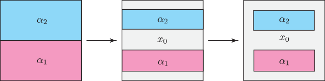
Figure 6: Shrinking the domains of the loops in such a way that the holonomy is not changed.

The reader is familiar with this deformation in the case $n=0$. Compute the holonomy $\operatorname{hol}(\gamma)$ for a loop $\gamma\in\Omega^{1}(M,x_{0})$. Consider the loop $\tilde{\gamma}$ which is the same point set as $\gamma$ but traversed in the following way: you stay at $x_{0}$ for $\tau\in[0,\pi/2]$, next you go fast along the same point set by setting $\tilde{\gamma}(\tau)=\gamma(2\tau-\pi)$ for $\tau\in[\pi/2,3\pi/2]$, and finally you stay at $x_{0}$ until $\tau$ reaches $2\pi$. This loop has the same holonomy for two reasons:(1) in part of the loop you are not moving hence $\partial x/\partial\tau=0$, and (2) the reparametrization invariance of the holonomy in the other part of the path.

We use the same idea as we go from the left diagram to the central one in Figure 6. We shrink the respective domains of the two loops in the $\tau$ direction exploiting the fact that at the beginning, middle and end we are at $x_{0}$. The holonomy is computed using eq. (2.1) but with connection $\mathcal{A}$. The same arguments presented in the block quote above are valid. This new loop has the same holonomy $\operatorname{hol}(\alpha_{2}\circ\alpha_{1})$. Next we move from the central diagram to the right diagram in Figure 6 by shrinking the domains in the $\sigma^{n}$ direction. Inspecting (2.20) we see that the connection is essentially unaltered because $\partial x/\partial\sigma^{n}=0$ in the extension parts and the automatically built in reparametrization invariance in the $\bm{\sigma}$ directions. This may be seen more concretely by studying the $n=1$ case of (2.3) and again noticing that $\partial x/\partial\sigma$ vanishes in the extension parts and the reparametrization invariance in $\sigma$. This deformation does not change the holonomy. We finish by sequentially shrinking the domains in $\sigma^{n-1},\sigma^{n-2},\ldots,\sigma^{1}$. Once there we can go to Figure 5 and move things around using reparametrization invariance and the fact that we have a $r$-flat connection. These diffeomorphisms do not change the holonomy because of the $r$-flatness of $\mathcal{A}$. We finish by undoing the domain shrinking. Throughout this entire procedure the holonomy has not changed and thus we conclude that $\operatorname{hol}(\alpha_{2}\circ\alpha_{1})=\operatorname{hol}(\alpha_{1}\circ\alpha_{2})$ and we are finished with the proof.

Theorem 2.14.

The holonomy group of a $r$-flat connection $\mathcal{A}$ on $\Omega^{n}(M,x_{0})$ is abelian.

Next we argue that there is an Ambrose-Singer type theorem in play here by using some of the theorems from Section 2.5 about $r$-flat connections on $\Omega^{n}(M,x_{0})$. We probe the local curvature $D_{A}B$ at some point $x\in M$ of the connection $\mathcal{A}$ in the following way. Pick a reference path from $x_{0}$ to $x$. Consider a “degenerate loop” in $\Omega^{n+1}(M,x_{0})$ that has collapsed to the reference path in analogy to the top diagram in Figure 1. Such a loop has trivial holonomy. Next, at the endpoint $x$ on the path, we blow up the loop make a small infinitesimal bulb. Note that the surface of the bulb is $(n+1)$ dimensional while the “interior” of the bulb is morally $(n+2)$ dimensional. The holonomy for this loop will be the parallel transport along the path of the $(n+2)$ form $D_{A}B$ evaluated on the small volume. Mimicking Ambrose and Singer we parallel transport all the $D_{A}B$ from all points back to the basepoint $x_{0}$. These span some linear subspace $\mathfrak{h}$ of $\mathfrak{g}$. This Lie algebra subspace represent the infinitesimal holonomy. The argument is analogous to what is done in the Ambrose-Singer Theorem. Take the loop and approximate it with many bulbs. The holonomy group is abelian and so we expect $\mathfrak{h}$ to be abelian and to also be the Lie algebra of the holonomy group. In other words, the curvature $D_{A}B$ is related to the Lie algebra of the holonomy group à la Ambrose and Singer. We have argued that $\mathfrak{h}$ is an abelian subalgebra of $\mathfrak{g}$ but we have not found an argument for why it should be an abelian ideal.

2.7 Flat connections and holonomy

We remind the reader about a standard theorem in the theory of connections. Assume $X$ is a manifold with a flat connection with structure group $G$. The holonomy of a flat connection gives a group homomorphism, i.e., a representation, $\rho:\pi_{1}(X,x_{0})\to G$ that characterizes the flat connection in the connected component of $X$ containing $x_{0}$. We can apply this to our loop space connections. Notice that the definition of the homotopy groups tell us that $\pi_{k}(\Omega^{n}(X,x_{0}))=\pi_{n+k}(X,x_{0})$.

Let $\mathcal{A}$ be a flat connection on $\Omega^{n}(M,x_{0})$, $n\geq 1$. This connection is automatically $r$-flat and therefore has abelian holonomy. Our loop space is not necessarily connected because $\pi_{0}(\Omega^{n}(M,x_{0}))=\pi_{n}(M,x_{0})$. We can now restrict to a single connected component of $\Omega^{n}(M,x_{0})$. After all, we are stuck in a connected component because we continuously develop in time. From the previous paragraph we see that the holonomy of the flat connection gives us a group homomorphism $\rho:\pi_{n+1}(M,x_{0})\to H_{x_{0}}$ where $H_{x_{0}}\subset G$ is the abelian holonomy group. Note that $\pi_{n+1}(M,x_{0})$ is abelian and therefore its image under $\rho$ must be abelian. This behavior is compatible with Theorem 2.14.

Theorem 2.15.

A flat connection on $\Omega^{n}(M,x_{0})$ gives a representation $\rho:\pi_{n+1}(M,x_{0})\to H_{x_{0}}$ where $H_{x_{0}}\subset G$ is the abelian holonomy group.

Why is this theorem important for us? In our method the conserved charges may be obtained by taking traces of the holonomy element.

In the familiar Lax-Zakharov-Shabat construction, corresponding to $n=0$ in this notation, a flat connection gives a map $\rho:\pi_{1}(M,x_{0})\to G$. For $M=S^{1}$ then we have a map $\rho:\mathbb{Z}\to G$ that determines the conserved quantities. The image of $\rho$ will be abelian.

The case $n\geq 1$ corresponds to a spatial manifold with $\dim M=n+1$ and for simplicity we take $M=S^{n+1}$. We see that a flat $\mathcal{A}$ connection gives a representation $\rho:\pi_{1}(\Omega^{n}(S^{n+1},x_{0})\to H_{x_{0}}$. We note that $\pi_{n+1}(S^{n+1},x_{0})\approx\mathbb{Z}$ and therefore we have a group homomorphism $\rho:\mathbb{Z}\to H_{x_{0}}$ just as in the Lax-Zakharov-Shabat case.

2.8 Nested loop space connections

The loop space connection structures we have been discussing can be generalized in the following way [18] to a nested construction. First we relax the loop space definition to toroidal loop spaces

$$\Omega^{n}(M,x_{0}) =\bigl{\{}f:\mathbb{T}^{n}\to M\;|\;f(0)=x_{0}\bigr{\}},$$

$$=\bigl{\{}f:[0,2\pi]^{n}\to M\;|\;f(0,\ldots,0)=x_{0}\bigr{\}}\,.$$ (2.26)

The notation in this Section is chosen to agree with the conventions of Section 3. Assume we are studying integrable models in a $(d+1)$-spacetime. We introduce a sequence of ordinary connections $A^{(1)},A^{(2)},\ldots,A^{(d)}$ associated with Lie algebras $\mathfrak{g}^{(1)},\mathfrak{g}^{(2)},\ldots,\mathfrak{g}^{(d)}$. We also introduce a sequence of differential forms $B^{(1)},B^{(2)},\ldots,B^{(d)}$ where $B^{(k)}$ is a $\mathfrak{g}^{(k)}$-valued $k$-form that transforms under the respective adjoint representation. We will use $(A^{(k)},B^{(k)})$ to define a new type of parallel transport on $\Omega^{k-1}(M,x_{0})$ that is a twisted version of the construction in Section 2.5.

There are now a variety of games you can play. For example, you can make all the loop space connections independent of each other. No new obvious phenomenon is seen here.

You can try something that is highly non-trivial. Assume all the Lie algebras fit inside a big Lie algebra $\mathfrak{g}$. Let $P^{(k)}$ be the ordinary parallel transport along paths associated with the ordinary connection $A^{(k)}$. Introduce a “twisted” parallel transport operator $\mathcal{P}^{(k+1)}$ on $\Omega^{k}(M,x_{0})$ defined by an inductive procedure. The parallel transport from the constant base loop $x_{0}$ to $\gamma\in\Omega^{k}(M,x_{0})$ will be denoted by $\mathcal{P}^{(k+1)}(\gamma)$. We recall that our toroidal loop spaces are given by maps on an appropriate hypercube. This hypercube has a natural Cartesian coordinate system that we will use in the construction. The inductive definition is

$$0 =\frac{d}{d\tau}\;\mathcal{P}^{(k+1)}$$

$$\quad+\left[\left(\mathcal{P}^{(k)}\right)^{-1}\left(\int_{0}^{2\pi}d\sigma^{k}\;\left(P^{(k+1)}\right)^{-1}\left(\iota_{\partial/\partial\sigma^{k}}\iota_{\partial/\partial\tau}B^{(k+1)}\right)P^{(k+1)}\right)\left(\mathcal{P}^{(k)}\right)\right]\mathcal{P}^{(k+1)}\,.$$ (2.27)

This equation is a bit schematic and requires some explanation. We start at $x_{0}$ at $\tau=0$ and we evolve in time $\tau$ to a loop $\gamma_{\tau}\in\Omega^{k}(M,x_{0})$. The developed surface is a $(k+1)$-submanifold $\Sigma_{\tau}$ with boundary $\partial\Sigma_{\tau}=\gamma_{\tau}-\{x_{0}\}$. We note that

$$\int_{0}^{2\pi}d\sigma^{k}\;\left(P^{(k+1)}\right)^{-1}\left(\iota_{\partial/\partial\sigma^{k}}\iota_{\partial/\partial\tau}B^{(k+1)}\right)P^{(k+1)}$$

is a $(k-1)$-form. At time $\tau$ and at location $(\sigma^{1},\sigma^{2},\ldots,\sigma^{k-1},\sigma^{k})$ the term above is sum of the parallel transports of $B^{(k+1)}$ using $A^{(k+1)}$ along the curves with tangent vector $\partial/\partial\sigma^{k}$ to the “boundary” with coordinates $(\sigma^{1},\sigma^{2},\ldots,\sigma^{k-1},0)$. This boundary is a loop $\gamma_{\tau}(\sigma^{1},\sigma^{2},\ldots,\sigma^{k-1},0)$ in $\Omega^{k-1}(M,x_{0})$ and therefore the Lie algebra element we have just computed can be parallel transported using $\mathcal{P}^{(k-1)}$. Some concrete examples are given in [18]. N.B. Had we used the spherical loop spaces then at the boundary $\gamma_{\tau}(\sigma^{1},\sigma^{2},\ldots,\sigma^{k-1},0)=x_{0}$ and what we are trying to do collapses and we are basically back in Section 2.5.

The upshot of the nested structure given by (2.27) is that $B^{(k)}$ at different levels can mix. We have not studied $r$-flatness in this case but imposing cross level vanishing of brackets as in (3.11) leads to conserved quantities.

3 The local zero curvature conditions

We now discuss the local conditions in space-time which are sufficient for the vanishing of the curvature of the connection on loop space.

As we have seen in the previous sections, the implementation of the generalized zero curvature condition in a space-time ${\cal M}$ of $d+1$ dimensions involves a nested structure of generalized loop spaces (see section 2.8). In order to define the one-form connection on loop space we introduced in the space-time ${\cal M}$, $d$ pairs of antisymmetric tensors $B_{\mu_{1}\ldots\mu_{N}}^{(N)}$ and one-form connections $A_{\mu}^{(N)}$, with $N=1,2,\ldots d$. The connections were used to parallel transport the tensors along curves starting and ending at a chosen fixed point $x_{0}$ of ${\cal M}$. Consequently, the tensors appear always in the conjugated form

$$B_{\mu_{1}\mu_{2}\ldots\mu_{N}}^{W_{N}}\equiv W_{N}^{-1}\,B_{\mu_{1}\mu_{2}\ldots\mu_{N}}^{(N)}\,W_{N}$$ (3.1)

where $W_{N}$ is obtained by integrating the connection along the curve, parameterized by $\sigma$, through the differential equation

$$\frac{dW_{N}}{d\sigma}+A_{\mu}^{(N)}\frac{dx^{\mu}}{d\sigma}W_{N}=0$$ (3.2)

In the previous sections we discussed the conditions for the connection on loop spaces to be $r$-flat. Here we shall impose in addition that the connections $A_{\mu}^{(N)}$ are flat, i.e.

$$F_{\mu\nu}^{(N)}\equiv\partial_{\mu}A_{\nu}^{(N)}-\partial_{\nu}A_{\mu}^{(N)}+\left[\,{A_{\mu}^{(N)}}\,,\,{A_{\nu}^{(N)}}\,\right]=0$$ (3.3)

That implies that the quantities $W_{N}$ are uniquely defined on every point of ${\cal M}$, once their values at $x_{0}$ are chosen. The connections are then written in the pure gauge form

$$A_{\mu}^{(N)}=-\partial_{\mu}W_{N}\,W_{N}^{-1}$$ (3.4)

As we have seen the generalized zero curvature condition does lead to conserved quantities expressed in terms of path ordered integrals of the connection on loop space. In $1+1$ dimensions the loop space coincides with (or is isomorphic to) the space-time ${\cal M}$, and so these non-locality problems disappear leading in fact to an extension of the usual formulation of two dimensional integrable theories given by the equations

$$\partial_{\mu}A_{\nu}^{(1)}-\partial_{\nu}A_{\mu}^{(1)}+\left[\,{A_{\mu}^{(1)}}\,,\,{A_{\nu}^{(1)}}\,\right]=0$$ (3.5)

and

$$D_{\mu}^{(1)}B_{\nu}^{(1)}-D_{\nu}^{(1)}B_{\mu}^{(1)}+\left[\,{B_{\mu}^{(1)}}\,,\,{B_{\nu}^{(1)}}\,\right]=0$$ (3.6)

where

$$D_{\mu}^{(N)}\bullet\equiv\partial_{\mu}\bullet+\left[\,{A_{\mu}^{(N)}}\,,\,{\bullet}\,\right]$$ (3.7)

The relation (3.5) is the usual Lax-Zakharov-Shabat equation [56] employed in two dimensional integrable field theories, and it leads to the conserved charges which are the eigenvalues of the path ordered integrals

$$W_{1}=P\,e^{\int_{\Gamma}d\sigma\,A_{\mu}^{(1)}\frac{dx^{\mu}}{d\sigma}}$$ (3.8)

where $\Gamma$ is the one dimensional space submanifold of the two dimensional space-time ${\cal M}$. However, our formulation also includes another vector $B_{\mu}^{(1)}$ satisfying (3.6) and that leads to another set of conserved quantities given by the eigenvalues of the operator

$$V_{1}=P\,e^{\int_{\Gamma}d\sigma\,W_{1}^{-1}\,B_{\mu}^{(1)}\,W_{1}\,\frac{dx^{\mu}}{d\sigma}}$$ (3.9)

The consequences of the existence of that second type of charges are now being investigated and may perhaps unify some treatments of local and non-local charges in two dimensional field theories [34].

The question we face in dimensions higher than two is how to relate the loop space zero curvature condition to the dynamics (equations of motion) of theories defined on the space-time ${\cal M}$. The main obstacle is the highly non-local character of the loop space zero curvature when expressed in terms of the tensors and connections defined in ${\cal M}$. That fact makes us believe that the proper formulation of integrable theories in a space-time of dimension higher than two may require not just terms involving particles but also terms that include fluxes or other extended objects. The implementation of such ideas is therefore the main challenge to our approach in the future.

However, one can avoid the non-locality problems of the zero curvature condition by selecting local equations in ${\cal M}$ which are sufficient conditions for the vanishing of the loop space curvature. We have seen in the previous sections that the concept of $r$-flatness leads to an improvement of such non-locality problems, since it implies the vanishing of the commutator term separately from the term involving the exterior covariant derivative of the tensors $B$’s (see Theorem 2.4). Therefore, one observes that one way (and perhaps the only one) of imposing local conditions on ${\cal M}$ which are sufficient for two conditions on loop space, namely the vanishing of the loop space zero curvature and its independence of the scanning of the hypersurfaces (i.e. $r$-flatness), is to have, in addition to (3.3), the covariant exterior derivative of the tensors $B^{(N)}$ equal to zero, i.e.

$$D^{(N)}\wedge B^{(N)}=0\qquad\qquad N=1,2\ldots d$$ (3.10)

with $D^{(N)}$ defined in (3.7), and in addition to have the commutators of the components of the tensors (3.1) also vanishing, i.e.

$$\left[\,{B_{\mu_{1}\mu_{2}\ldots\mu_{N}}^{W_{N}}}\,,\,{B_{\nu_{1}\nu_{2}\ldots\nu_{M}}^{W_{M}}}\,\right]=0\qquad\qquad M,N=1,2\ldots d$$ (3.11)

The relations (3.3), (3.10) and (3.11) are what we call the sufficient local zero curvature conditions. They indeed lead to conserved quantities as we now explain. From (3.4) and (3.10) one obtains that the ordinary exterior derivative of $B_{\mu_{1}\mu_{2}\ldots\mu_{N}}^{W_{N}}$ vanishes, i.e

$$d\wedge B^{W_{N}}=0$$ (3.12)

It then follows that if $V_{N+1}$ is a $N+1$-dimensional volume in ${\cal M}$, and $\partial V_{N+1}$ is its boundary, i.e. a $N$-dimensional closed surface, then by (3.12) and the abelian Stokes theorem

$$\int_{\partial V_{N+1}}B^{W_{N}}=\int_{V_{N+1}}d\wedge B^{W_{N}}=0$$ (3.13)

Notice that, if $B^{W_{N}}$ lives on a vector space with basis $v^{a}$, we are applying the abelian Stokes theorem to each component $B^{W_{N}}_{a}$ separately ($B^{W_{N}}_{\mu_{1}\ldots\mu_{N}}=B^{W_{N}}_{\mu_{1}\ldots\mu_{N};a}\,v^{a})$, and the issue if those components commute among themselves is not relevant here. Imposing appropriate boundary conditions on the pair $\left(A^{(N)},B^{(N)}\right)$ can lead to conservation laws as we now explain. In a space-time ${\cal M}$ of $d+1$ dimensions, there are $d-N+1$ orthogonal directions to a $N$-dimensional surface. Let us choose one of those directions and let us parametrize it by $\tau$. We can choose the volume $V_{N+1}$ such that its border can be decomposed as

$$\partial V_{N+1}=\Sigma_{N}^{\tau_{0}}+\Sigma_{N}^{\tau_{1}}+\Gamma_{N}$$ (3.14)

where $\Sigma_{N}^{\tau_{0}}$ and $\Sigma_{N}^{\tau_{1}}$ are $N$ dimensional surfaces perpendicular to the direction $\tau$, and corresponding to fixed values $\tau_{0}$ and $\tau_{1}$ respectively, of the parameter $\tau$. $\Gamma_{N}$ is a $N$ dimensional surface joining $\Sigma_{N}^{\tau_{0}}$ and $\Sigma_{N}^{\tau_{1}}$ into the closed surface $\partial V_{N+1}$. If the boundary conditions are such that the integral of $B^{W_{N}}$ on $\Gamma_{N}$ vanishes we then have from (3.13) and (3.14) that

$$\int_{\Sigma_{N}^{\tau_{0}}}B^{W_{N}}+\int_{\Sigma_{N}^{\tau_{1}}}B^{W_{N}}=0$$ (3.15)

If one now orients the surfaces in the same way with respect to the $\tau$ direction one has a conserved charge in $\tau$ given by

$$Q^{(N)}=\int_{\Sigma_{N}}\,B^{W_{N}}$$ (3.16)

where $\Sigma_{N}$ is any surface perpendicular to the $\tau$ direction. Of course, we will be mainly interested in quantities conserved in time and so we will be concerned most with the case $N=d$, with $\Sigma_{N}$ being the spatial sub-manifold the space-time ${\cal M}$. In any case, the number of conserved charges will be determined by the dimension of the space where the tensors $B^{(N)}$ live.

We notice that the Hodge dual of $B^{W_{N}}$ in the $d+1$ dimensional space-time ${\cal M}$, i.e.

$$J^{\rho\mu_{1}\ldots\mu_{d-N}}\equiv\varepsilon^{\rho\mu_{1}\ldots\mu_{d-N}\nu_{1}\ldots\nu_{N}}\,B_{\nu_{1}\nu_{2}\ldots\nu_{N}}^{W_{N}}$$ (3.17)

is, as a consequence of (3.12), a conserved antisymmetric tensor

$$\partial_{\rho}\,J^{\rho\mu_{1}\ldots\mu_{d-N}}=0$$ (3.18)

and that is another way of expressing the conservation law we just discussed.

Note that associated to every pair $\left(B_{\mu_{1}\ldots\mu_{N}}^{(N)},A_{\mu}^{(N)}\right)$, we have gauge symmetries of the sufficient local zero curvature conditions (3.3), (3.10), and (3.11). Consider the transformations

$$A_{\mu}^{(N)} \rightarrow g\,A_{\mu}^{(N)}\,g^{-1}-\partial_{\mu}g\,g^{-1}$$

$$B_{\mu_{1}\ldots\mu_{N}}^{(N)} \rightarrow g\,B_{\mu_{1}\ldots\mu_{N}}^{(N)}\,g^{-1}$$ (3.19)

where $g$ is an element in a group with the Lie algebra corresponding to where the connection $A_{\mu}^{(N)}$ lives, and $g$ acts on the tensor $B_{\mu_{1}\ldots\mu_{N}}^{(N)}$. It then follows that the covariant derivatives of $B_{\mu_{1}\ldots\mu_{N}}^{(N)}$ transform in the same way

$$D_{\nu}^{(N)}B_{\mu_{1}\ldots\mu_{N}}^{(N)}\rightarrow g\,D_{\nu}^{(N)}B_{\mu_{1}\ldots\mu_{N}}^{(N)}\,g^{-1}.$$ (3.20)

Therefore, (3.3) and (3.10) are clearly invariant under (3.19). In addition, we have that under (3.19)

$$W_{N}\rightarrow g\left(x\right)\,W_{N}\,g^{-1}\left(x_{0}\right)$$ (3.21)

where $x_{0}$ and $x$ are the initial and final points respectively, of the curve where $W_{N}$ is calculated, with $x_{0}$ being the fixed point of ${\cal M}$ we introduced above. Consequently, $B_{\mu_{1}\ldots\mu_{N}}^{W_{N}}$ is invariant under (3.19), and so is the condition (3.11). It also follows that the conserved charges (3.16) are invariant under (3.19).

The covariant derivatives (3.7) commute since the connections $A_{\mu}^{(N)}$ are flat, and so most of the properties of the ordinary exterior derivatives apply as well as to covariant exterior derivatives, in particular $D^{2}=0$. Therefore, the conditions (3.3) and (3.10) are invariant under the gauge transformations

$$A^{(N)} \rightarrow A^{(N)}$$ (3.22)

$$B^{(N)} \rightarrow B^{(N)}+D^{(N)}\wedge\alpha^{(N-1)}$$

where $\alpha^{(N-1)}$ is an antisymmetric tensor of rank $N-1$. The invariance of the condition (3.11) under (3.22) needs some more refined structures which we discuss below.

Basically there are two ways of implementing the conditions (3.10) and (3.11). The first one is as follows. Given the reference point $x_{0}$ of ${\cal M}$ we take the components of the tensors $B^{(N)}$ on that point to commute, i.e.

$$\left[\,{B^{(N)}_{\mu_{1}\ldots\mu_{N}}\left(x_{0}\right)}\,,\,{B^{(N)}_{\nu_{1}\ldots\nu_{N}}\left(x_{0}\right)}\,\right]=0$$ (3.23)

Then we use the fact that the connections $A_{\mu}^{(N)}$ are flat (see (3.4)) and construct the tensors $B^{(N)}$ on any point $x$ of ${\cal M}$, by parallel transport with the connection $A_{\mu}^{(N)}$ along a given curve from the fixed point $x_{0}$ to $x$. Notice that since the connections are flat it does not matter the curve we choose to link $x_{0}$ to $x$. We then have that

$$B^{(N)}_{\mu_{1}\ldots\mu_{N}}=W_{N}\,B^{(N)}_{\mu_{1}\ldots\mu_{N}}\left(x_{0}\right)\,W_{N}^{-1}$$ (3.24)

Consequently, from (3.1) one has

$$B_{\mu_{1}\mu_{2}\ldots\mu_{N}}^{W_{N}}=B^{(N)}_{\mu_{1}\ldots\mu_{N}}\left(x_{0}\right)$$ (3.25)

and so (3.11) is satisfied. Of course, such tensors are covariantly constant

$$D^{(N)}_{\nu}B^{(N)}_{\mu_{1}\ldots\mu_{N}}=0$$ (3.26)

and so they trivially satisfy (3.10). Notice that (3.23) and (3.24) imply that the components of the tensors $B^{(N)}_{\mu_{1}\ldots\mu_{N}}$ commute on every point on ${\cal M}$. However, those components at different points do not have to do so.

The invariance of the condition (3.11) under (3.22) can be established by taking $\alpha^{(N-1)}$ as the parallel transport of a tensor $\alpha^{(N-1)}_{0}$, in a way similar to (3.24), i.e.

$$\alpha^{(N-1)}=W_{N}\,\alpha^{(N-1)}_{0}\,W_{N}^{-1}$$ (3.27)

We then have $D^{(N)}\wedge\alpha^{(N-1)}=W_{N}\,d\wedge\alpha^{(N-1)}_{0}\,W_{N}^{-1}$, and if we impose that $d\wedge\alpha^{(N-1)}_{0}$ live in the same abelian algebra as the components of $B^{(N)}_{\mu_{1}\ldots\mu_{N}}\left(x_{0}\right)$ (see (3.23)), we have the invariance of (3.11) under (3.22).

The conserved charges (3.16) in such case have a geometrical meaning and correspond to projections of hypersurfaces in the directions defined by those constant tensors. Indeed, from (3.16) and (3.25) one has

$$Q^{N}=\int_{\Sigma_{N}}\,B^{W_{N}}=B^{(N)}_{\mu_{1}\ldots\mu_{N}}\left(x_{0}\right)\,\int_{\Sigma_{N}}\,d\Sigma^{\mu_{1}\ldots\mu_{N}}$$ (3.28)

The examples we found that fit in the first type of local zero curvature condition are topological field theories like Chern-Simons and BF theories. Indeed, the BF theory in $2+1$ dimensions [30] involves an antisymmetric tensor $B_{\mu\nu}$ and a flat connection $A_{\mu}$, and its equations of motion are given by (3.3) and (3.26) for $N=2$. Obviously, the Chern-Simons theory also fits into the scheme since it involves just a flat connection. We believe however that the important applications of our methods to topological theories will appear when we consider our loop spaces defined on space-times ${\cal M}$ with non-trivial topological structures like holes, handles, etc. We will then have to use modifications of the non-abelian Stoke’s theorem on loop space on the lines of [52]. In the case of Chern-Simons and BF theories we may perhaps relate the modification of our conserved quantities (3.28) to the knot theory invariants which are known to appear in those models.

A second way of implementing the local conditions (3.10) and (3.11) involves taking the pairs $\left(B_{\mu_{1}\ldots\mu_{N}}^{(N)},A_{\mu}^{(N)}\right)$ to live in a non-semisimple Lie algebra ${\cal G}^{(N)}$, such that $B_{\mu_{1}\ldots\mu_{N}}^{(N)}$ has components only in the direction of the abelian ideal ${\cal P}^{(N)}$ of ${\cal G}^{(N)}$. It then follows that $W_{N}$ belongs to the group whose Lie algebra is ${\cal G}^{(N)}$ and therefore $B_{\mu_{1}\mu_{2}\ldots\mu_{N}}^{W_{N}}$, defined in (3.1), also belongs to the abelian ideal ${\cal P}^{(N)}$. If we now impose that the different abelian ideals commute

$$\left[\,{{\cal P}^{(M)}}\,,\,{{\cal P}^{(N)}}\,\right]=0\qquad\qquad M,N=1,2\ldots d$$ (3.29)

then we satisfy condition (3.11). The equation (3.10) is then the only condition to be imposed on the tensors $B^{(N)}$ and it will therefore define the dynamics of the generalized integrable theory as specified below. Notice that such formulation does not need to specify the commutation relations among the complements of the ${\cal P}^{(N)}$s in the algebras ${\cal G}^{(N)}$s. The number of conserved charges coming from (3.16) is of course given by the sum of the dimensions of the abelian ideals ${\cal P}^{(N)}$, where the tensors $B^{(N)}$ live.

The invariance of the condition (3.11) under (3.22) is guaranteed by taking the tensors $\alpha^{(N-1)}$ to live in the abelian ideals ${\cal P}^{(N)}$.

We then observe that the algebraic structure underlying that second type of local integrable theories is that of non-semisimple Lie algebras. Most of those algebras can be cast in terms of a semi-simple Lie algebra ${\cal G}$ and a representation $R$ of it, with the commutation relations being given by

$$\left[\,{T_{a}}\,,\,{T_{b}}\,\right] = f_{ab}^{c}\,T_{c}$$

$$\left[\,{T_{a}}\,,\,{P_{i}}\,\right] = P_{j}\,R_{ji}\left(T_{a}\right)$$ (3.30)

$$\left[\,{P_{i}}\,,\,{P_{j}}\,\right] = 0$$

with $R$ being a matrix representation of ${\cal G}$, i.e.

$$\left[\,{R\left(T_{a}\right)}\,,\,{R\left(T_{b}\right)}\,\right]=R\left(\left[\,{T_{a}}\,,\,{T_{b}}\,\right]\right)$$ (3.31)

Therefore, since the number of conserved currents is given by the dimension of the abelian ideal ${\cal P}$, it follows that the integrability concepts will be related to infinite dimensional representations. As we will see in the applications, those representations will be given in general by infinite direct products of finite representations, i.e. $R=\otimes_{k}R_{k}$. This differs in a crucial way from the algebraic structures we find in $1+1$ dimensional integrable theories where we have infinite algebras like the Kac-Moody algebras. Such algebras can in fact be graded as

$${\hat{\cal G}}=\otimes_{n=-\infty}^{\infty}{\hat{\cal G}}_{n}\qquad\qquad\left[\,{{\hat{\cal G}}_{m}}\,,\,{{\hat{\cal G}}_{n}}\,\right]\subset{\hat{\cal G}}_{m+n}$$ (3.32)

The subspace ${\hat{\cal G}}_{0}$ is a finite subalgebra and the other subspaces transform under a given representation of it $\left[\,{{\hat{\cal G}}_{0}}\,,\,{{\hat{\cal G}}_{n}}\,\right]\subset{\hat{\cal G}}_{n}$, similarly to the ideals ${\cal P}$ under ${\cal G}$. However, the crucial difference with our formulation is that the generators in those representations do not have to commute. The requirement of locality is what has driven us to the abelian character of those representations. In order to have the full algebraic structures of the zero curvature condition on loop spaces, we believe we have to deal with theories where the fundamental objects are not just particles but perhaps fluxes.

The second way of implementing local conditions that imply the vanishing of the loop space zero curvature shows that the relation (3.11) is satisfied by an algebraic procedure and so it does not lead to conditions on the dynamics of the theory. Such conditions have to come from the relations (3.3) and (3.10). In the applications of such formulations for Lorentz invariant theories that have appeared in the literature so far, only the pair $\left(A^{(N)},B^{(N)}\right)$ for $N=d$ has been used. In such cases the Hodge dual of $B^{(N)}$ is a vector, i.e.

$${\tilde{B}}^{\mu}\equiv\varepsilon^{\mu\nu_{1}\ldots\nu_{d}}\,B^{(N=d)}_{\nu_{1}\ldots\nu_{d}}.$$ (3.33)

Therefore, the condition (3.10) becomes

$$D_{\mu}{\tilde{B}}^{\mu}=0$$ (3.34)

We then have from (3.17) the conserved currents

$$J^{\mu}=W^{-1}_{N=d}\,{\tilde{B}}^{\mu}\,W_{N=d}\qquad\qquad\qquad\partial_{\mu}J^{\mu}=0$$ (3.35)

In the examples constructed in the literature thus far, the equations of motion were found to be equivalent to the condition (3.34) (or (3.10)), whilst the condition (3.3) was trivially satisfied, i.e. involved a connection that was flat for any field configuration. For theories that are not Lorentz invariant there are examples where the equations of motion come from (3.3) and where (3.10) was trivially satisfied, i.e. the tensors $B^{(N=d)}$ were the exterior covariant derivative of a lower rank tensor, i.e. $B^{(N=d)}=D^{(N=d)}\wedge\alpha^{(d-1)}$. We now discuss some examples where this formulation was implemented.

4 Examples

4.1 Models on the sphere $S^{2}$

A class of models that has been well explored using the formulation described in Section 3 is one where the fields take values on the two dimensional sphere $S^{2}$. The fields may be taken to be a triplet of real scalar fields ${\vec{n}}$ subject to the constraint ${\vec{n}}^{2}=1$, or alternatively a complex scalar field $u$ parametrizing the plane that corresponds to the stereographic projection of $S^{2}$. The two descriptions are related by

$${\vec{n}}=\frac{1}{1+\mid u\mid^{2}}\,\left(u+u^{*},-i\left(u-u^{*}\right),\mid u\mid^{2}-1\right)\qquad\quad u=\frac{n_{1}+i\,n_{2}}{1-n_{3}}$$ (4.1)

In the examples discussed in the literature thus far only the pair $\left(A^{(N)},B^{(N)}\right)$, for $N=d$ has been used (with $d$ being the number of space dimensions). The flat connection, satisfying (3.3), is taken to live in the algebra of $sl(2)$ and given by [18]

$$A_{\mu}^{(d)}\equiv A_{\mu}=\frac{1}{1+\mid u\mid^{2}}\left[-i\partial_{\mu}uT_{+}-i\partial_{\mu}u^{*}T_{-}+\left(u\,\partial_{\mu}u^{*}-u^{*}\,\partial_{\mu}u\right)\,T_{3}\right]$$ (4.2)

with the generators satisfying the $sl(2)$ commutation relations

$$[T_{3},T_{\pm}]=\pm T_{\pm}\;\qquad\qquad[T_{+},T_{-}]=2T_{3}$$ (4.3)

Notice that such a connection is flat and satisfies (3.3) for any configuration of the complex field $u$. In fact, you can write the connection in the pure gauge form (3.4) with $W_{N=d}\equiv W_{i}$, $i=1,2$, and

$$W_{1}=e^{iuT_{+}}\,e^{\varphi T_{3}}\,e^{iu^{*}T_{-}}\,;\qquad\qquad\qquad W_{2}=e^{iu^{*}T_{-}}\,e^{-\varphi T_{3}}\,e^{iuT_{+}}$$ (4.4)

where $\varphi=\ln(1+\mid u\mid^{2})$. Notice that $W_{1}$ and $W_{2}$ are elements of the group $SL(2,\mathbb{C})$, and not of $SU(2)$, but $iA_{\mu}$ does belong to the algebra of $SU(2)$. The commutation relations (4.3) are compatible with the hermiticity conditions, $T_{3}^{\dagger}=T_{3}$, $T_{\pm}^{\dagger}=T_{\mp}$, and so $W_{1}^{\dagger}=W_{2}^{-1}$. In the defining (spinor) representation $R^{(1/2)}$ of $SL(2,\mathbb{C})$ one has that the elements $W_{1}$ and $W_{2}$ coincide, i.e.

$$W\equiv R^{(1/2)}\left(W_{1}\right)=R^{(1/2)}\left(W_{2}\right)={1\over{\sqrt{1+\mid u\mid^{2}}}}\,\left(\begin{array}[]{cc}1&iu\\ iu^{*}&1\end{array}\right)$$ (4.7)

Therefore, they are unitary two by two matrices of unity determinant and so elements of $SU(2)$.

Another interesting point is that the sphere $S^{2}$ can be mapped isometrically into the symmetric space $SU(2)/U(1)$ that may be identified with the complex projective space $CP^{1}$. The $U(1)$ subgroup is invariant under the involutive automorphism of the algebra (4.3)

$$\sigma\left(T_{3}\right)=T_{3}\qquad\qquad\sigma\left(T_{\pm}\right)=-T_{\pm}$$ (4.8)

The automorphism (4.8) is inner and given by

$$\sigma\left(T\right)\equiv e^{i\pi T_{3}}\,T\,e^{-i\pi T_{3}}$$ (4.9)

The elements of $SU(2)/U(1)$ can be parametrized by the variable $x\left(g\right)\equiv g\sigma\left(g\right)^{-1}$, $g\in SU(2)$, since $x\left(g\right)=x\left(gk\right)$ with $k\in U(1)$. In addition one has that $\sigma\left(x\right)=x^{-1}$. In the spinor representation one has

$$R^{(1/2)}\left(e^{i\pi T_{3}}\right)=\left(\begin{array}[]{cc}i&0\\ 0&-i\end{array}\right)$$ (4.12)

and so $W$ defined in (4.7) satisfies.

$$\sigma\left(W\right)=W^{-1}$$ (4.13)

Therefore, $W$ takes the place of the variable $x\left(g\right)$, and so parametrizes the elements of the symmetric space $SU(2)/U(1)$, or equivalently of the sphere $S^{2}$ [20].

The other element in the pair, namely $B^{(d)}$, has to live in an abelian ideal, and so transform under some representation of $sl(2)$ (see discussion leading to (3.30)). Since we want models with an infinite number of conserved charges we must work with infinite dimensional representations. One way of doing that is to use the Schwinger’s construction. Let $R\left(T\right)$ be a (finite) matrix representation of the algebra $T$, i.e.

$$\left[\,{R\left(T\right)}\,,\,{R\left(T^{\prime}\right)}\,\right]=R\left(\left[\,{T}\,,\,{T^{\prime}}\,\right]\right)$$ (4.14)

Consider oscillators in equal numbers to the dimension of $R$,

$$\left[\,{a_{i}}\,,\,{a_{j}}\,\right]=0\qquad\left[\,{a_{i}^{\dagger}}\,,\,{a_{j}^{\dagger}}\,\right]=0\qquad\left[\,{a_{i}}\,,\,{a_{j}^{\dagger}}\,\right]=\delta_{ij}\qquad\quad i,j=1,\ldots{\rm dim}\;R$$ (4.15)

It follows that the operators

$$S\left(T\right)\equiv\sum_{i,j}a^{\dagger}_{i}R_{ij}\left(T\right)a_{j}$$ (4.16)

constitute a representation of $T$

$$\left[\,{S\left(T\right)}\,,\,{S\left(T^{\prime}\right)}\,\right]=S\left(\left[\,{T}\,,\,{T^{\prime}}\,\right]\right)$$ (4.17)

The oscillators can be realized in terms of differential operators on some variables $\lambda_{i}$, as $a_{i}\equiv\frac{\partial\;}{\partial\lambda_{i}}$ and $a_{i}^{\dagger}=\lambda_{i}$. In the case of the algebra (4.3), one gets that its two dimensional matrix representation leads to the following realization in terms of differential operators (with the parameters $\lambda_{i}$, $i=1,2$, being denoted $\lambda$ and $\bar{\lambda}$) [24]

$$S\left(T_{+}\right)\equiv\lambda\,\frac{d\;}{d\bar{\lambda}}\;;\qquad S\left(T_{-}\right)\equiv\bar{\lambda}\,\frac{d\;}{d\lambda}\;;\qquad S\left(T_{3}\right)\equiv\frac{1}{2}\left(\lambda\,\frac{d\;}{d\lambda}-\bar{\lambda}\,\frac{d\;}{d\bar{\lambda}}\right)$$ (4.18)

The states of the representations corresponding to such realization are functions of $\lambda$ and $\bar{\lambda}$. The action of the operators are given by

$$S\left(T_{3}\right)\lambda^{p}\,\bar{\lambda}^{q} = \frac{p-q}{2}\,\lambda^{p}\,\bar{\lambda}^{q}$$

$$S\left(T_{+}\right)\lambda^{p}\,\bar{\lambda}^{q} = q\,\lambda^{p+1}\,\bar{\lambda}^{q-1}$$

$$S\left(T_{-}\right)\lambda^{p}\,\bar{\lambda}^{q} = p\,\lambda^{p-1}\,\bar{\lambda}^{q+1}$$ (4.19)

Notice that from (4.19) that the action of $S\left(T_{3}\right)$ and $S\left(T_{\pm}\right)$ leaves the sum of the powers of $\lambda$ and ${\bar{\lambda}}$ invariant. Therefore, one can construct irreducible representations by considering the states

$$\left\lvert\left(p,q\right),m\right\rangle\equiv\lambda^{p+m}\,\bar{\lambda}^{q-m}$$ (4.20)

with $m\in\mathbb{Z}$ and $\left(p,q\right)$ being any pair of numbers (real or even complex). Then

$$S\left(T_{3}\right)\left\lvert\left(p,q\right),m\right\rangle = \left(\frac{p-q}{2}+m\right)\,\left\lvert\left(p,q\right),m\right\rangle$$

$$S\left(T_{+}\right)\left\lvert\left(p,q\right),m\right\rangle = \left(q-m\right)\,\left\lvert\left(p,q\right),m+1\right\rangle$$

$$S\left(T_{-}\right)\left\lvert\left(p,q\right),m\right\rangle = \left(p+m\right)\,\left\lvert\left(p,q\right),m-1\right\rangle$$ (4.21)

On the subspace with fixed $(p+q)$, the Casimir operator acts as:

$$\left[S\left(T_{3}\right)^{2}+{1\over 2}\bigl{(}S\left(T_{+}\right)S\left(T_{-}\right)+S\left(T_{-}\right)S\left(T_{+}\right)\bigr{)}\right]\left\lvert\left(p,q\right),m\right\rangle=s(s+1)\left\lvert\left(p,q\right),m\right\rangle$$

with $s={1\over 2}(p+q)$. The parameter $s$ is the spin of the representation.

From the relations (4.21) one notices that if $p$ is an integer, then $\left\lvert\left(p,q\right),-p\right\rangle$ is a lowest weight state, since it is annihilated by $S\left(T_{-}\right)$. Analogously, if $q$ is an integer, then $\left\lvert\left(p,q\right),q\right\rangle$ is a highest weight state. If $p$ and $q$ are integers and $q>-p$, then the irrep. is finite dimensional. In order to have integer spin representations we need $\frac{p-q}{2}\in\mathbb{Z}$. The spin zero state is $\left\lvert\left(p,q\right),-\frac{p-q}{2}\right\rangle=\left(\lambda\,\bar{\lambda}\right)^{\frac{p+q}{2}}$. Notice however, that not all irreps. for integer spin will have the zero spin state. The reason is that if $p$ is a negative integer, or $q$ is a positive integer, then the representation will truncate before reaching the zero spin state.

In the $\lambda-{\bar{\lambda}}$ representations (4.18) the potential (4.2) becomes

$$A_{\mu}\equiv\frac{1}{1+\mid u\mid^{2}}\left(-i\partial_{\mu}u\lambda\frac{d\;}{d\bar{\lambda}}-i\partial_{\mu}u^{*}\bar{\lambda}\frac{d\;}{d\lambda}+\left(u\partial_{\mu}u^{*}-u^{*}\partial_{\mu}u\right)\frac{1}{2}\left(\lambda\,\frac{d\;}{d\lambda}-\bar{\lambda}\,\frac{d\;}{d\bar{\lambda}}\right)\right)$$ (4.22)

In a space-time of $d+1$ dimensions the Hodge dual of the rank $d$ antisymmetric tensor $B^{(N=d)}_{\mu_{1}\ldots\mu_{d}}$ is a vector, as given in (3.33). We shall introduce such dual vector in a spin $s$ representation of the algebra (4.3) as

$${\tilde{B}}_{\mu}^{(s)}\equiv\frac{1}{1+\mid u\mid^{2}}\left({\cal K}_{\mu}\lambda^{s+1}\bar{\lambda}^{s-1}-{\cal K}_{\mu}^{*}\lambda^{s-1}\bar{\lambda}^{s+1}\right)$$ (4.23)

where the vector ${\cal K}_{\mu}$ can be a priori any functional of $u$, $u^{*}$ and their derivatives. Notice that we have chosen $B_{\mu}^{(s)}$ to live in a representation where $p=q=s$, and it has components only in the direction of the states with eigenvalues $\pm 1$ of $T_{3}$.

As we have seen, the connection (4.22) (or (4.2)) is flat for any configuration of the field $u$. In addition, the condition (3.11) is satisfied because the tensors $B^{W_{d}}$ live in an abelian ideal, namely that generated by functions of the parameters $\lambda$ and ${\bar{\lambda}}$ (see (4.23)). Therefore, the only local condition to be satisfied is (3.34) (or (3.10)), i.e.

$$D^{\mu}{\tilde{B}}_{\mu}^{(s)}=\partial^{\mu}{\tilde{B}}_{\mu}^{(s)}+\left[\,{A^{\mu}}\,,\,{{\tilde{B}}_{\mu}^{(s)}}\,\right]=0$$ (4.24)

Therefore the equations of motion for the field $u$ come from the condition (4.24), and they depend of course on the choice of the spin $s$ of the representation.

For $s=1$, one gets that (4.24) implies the equations

$$\left(1+\mid u\mid^{2}\right)\,\partial^{\mu}{\cal K}_{\mu}-2\,u^{*}\,\partial^{\mu}u\,{\cal K}_{\mu}=0\qquad\qquad\partial^{\mu}u\,{\cal K}_{\mu}^{*}-\partial^{\mu}u^{*}\,{\cal K}_{\mu}=0$$ (4.25)

together with the complex conjugate of the first one.

For $s=-1$, (4.24) implies instead

$$\partial^{\mu}{\cal K}_{\mu}=0\qquad\qquad\partial^{\mu}u\,{\cal K}_{\mu}=0$$ (4.26)

together with their complex conjugates.

For $s\neq\pm 1$, one gets from (4.24)

$$\partial^{\mu}{\cal K}_{\mu}=0\qquad\qquad\partial^{\mu}u\,{\cal K}_{\mu}=0\qquad\qquad\partial^{\mu}u\,{\cal K}_{\mu}^{*}-\partial^{\mu}u^{*}\,{\cal K}_{\mu}=0$$ (4.27)

together with the complex conjugates of the first two equations.

The conserved charges following from (4.24) are those given in (3.16) for the case $N=d$, and with $\Sigma_{N}$ corresponding to the $d$ dimensional subspace of the space-time ${\cal M}$, orthogonal to the time direction. These charges are conserved in time and the corresponding conserved currents are given by (3.35), i.e.

$$J_{\mu}^{\left(s\right)}=W^{-1}_{j}\,{\tilde{B}}_{\mu}^{(s)}\,W_{j}$$ (4.28)

with $W_{j}$, $j=1,2$, being given in (4.4). The fact that the two group elements $W_{1}$ and $W_{2}$ give the same currents can be checked by explicit calculations. Indeed, using (4.18) one has that, for an arbitrary function $f\left(\lambda,{\bar{\lambda}}\right)$,

$$e^{\alpha S\left(T_{+}\right)}f\left(\lambda,\bar{\lambda}\right)e^{-\alpha S\left(T_{+}\right)} = f\left(\lambda,\bar{\lambda}+\alpha\lambda\right)$$

$$e^{\beta S\left(T_{-}\right)}f\left(\lambda,\bar{\lambda}\right)e^{-\beta S\left(T_{-}\right)} = f\left(\lambda+\beta\bar{\lambda},\bar{\lambda}\right)$$

$$e^{\gamma S\left(T_{3}\right)}f\left(\lambda,\bar{\lambda}\right)e^{-\gamma S\left(T_{3}\right)} = f\left(e^{\gamma/2}\lambda,e^{-\gamma/2}\bar{\lambda}\right)$$ (4.29)

Then you can check that

$$W_{j}^{-1}f\left(\lambda,\bar{\lambda}\right)W_{j}=f\left(\frac{\lambda-iu^{*}\bar{\lambda}}{\sqrt{1+\mid u\mid^{2}}},\frac{\bar{\lambda}-iu\lambda}{\sqrt{1+\mid u\mid^{2}}}\right)\qquad j=1,2$$ (4.30)

So, the two group elements give the same rotation on the parameters. Notice they look like a Lorentz boost on the space $\left(\lambda,\bar{\lambda}\right)$ and with complex velocity $iu$.

The models defined by the equations (4.25), corresponding to the case $s=1$, have only three conserved currents (4.28) and they are given by the three components of

$$J_{\mu}^{\left(1\right)}=\frac{{\cal K}_{\mu}+u^{2}\,{\cal K}_{\mu}^{*}}{\left(1+\mid u\mid^{2}\right)^{2}}\;\lambda^{2}-2\,i\,\frac{u^{*}\,{\cal K}_{\mu}-u\,{\cal K}_{\mu}^{*}}{\left(1+\mid u\mid^{2}\right)^{2}}\;\lambda\,{\bar{\lambda}}-\frac{{\cal K}_{\mu}^{*}+{u^{*}}^{2}\,{\cal K}_{\mu}}{\left(1+\mid u\mid^{2}\right)^{2}}\;{\bar{\lambda}}^{2}$$ (4.31)

Now, the models defined by the equations (4.26) corresponding to $s=-1$, have instead an infininte number of conserved currents. Indeed, one can check that

$$J_{\mu}^{\left(-1\right)}=\frac{{\cal K}_{\mu}}{\left({\bar{\lambda}}-i\,u\,\lambda\right)^{2}}-\frac{{\cal K}_{\mu}^{*}}{\left(\lambda-i\,u^{*}\,{\bar{\lambda}}\right)^{2}}$$ (4.32)

So, expanding in powers of $\lambda$ and ${\bar{\lambda}}$ one gets an infinite number of currents.

The models given by equations (4.27) have a much larger set of conserved currents since they admit a zero curvature representation for any spin $s$. Looking at eq. (4.23), we see that

$${\tilde{B}}_{\mu}^{\left(s\right)}=(\lambda\bar{\lambda})^{(s+1)}{\tilde{B}}_{\mu}^{\left(-1\right)}$$

If we consider a general ${\tilde{B}}_{\mu}=\sum_{s}\beta_{s}{\tilde{B}}_{\mu}^{\left(s\right)}$, we have

$${\tilde{B}}_{\mu}=b(\lambda\bar{\lambda}){\tilde{B}}_{\mu}^{\left(-1\right)}$$

where $b(z)=\sum_{s}\beta_{s}z^{s+1}$ is essentially an arbitrary function.

At the level of currents, this means

$$J_{\mu}=b\left({(\lambda-iu^{*}\bar{\lambda})(\bar{\lambda}-iu\lambda)\over 1+uu^{*}}\right)J_{\mu}^{\left(-1\right)}$$

We can write this in the nice form [20, 21, 48]:

$$J_{\mu}={\cal K}_{\mu}{\delta G\over\delta u}-{\cal K}^{*}_{\mu}{\delta G\over\delta u*}$$ (4.33)

where

$$G=i\int^{v(u,u^{*})}{dv\over v^{2}}\,b(v),\qquad\qquad v(u,u^{*})={(\lambda-iu^{*}\bar{\lambda})(\bar{\lambda}-iu\lambda)\over 1+uu^{*}}$$

Essentially $G$ is an arbitrary functional of $u$ and $u^{*}$, but not of its derivatives, and we have a conserved current for every $G$.

A large number of theories have been studied in the literature using the local zero curvature formulation we have just presented. We list here some examples.

4.1.1 The $CP^{1}$ model

The equations of motion are given by

$$\left(1+\mid u\mid^{2}\right)\partial^{2}u-2\,u^{*}\,\partial^{\mu}u\,\partial_{\mu}u=0$$ (4.34)

together with its complex conjugate. In such case we have ${\cal K}_{\mu}\equiv\partial_{\mu}u$, and so the first equation in (4.25) corresponds to (4.34), and the second is trivially satisfied.

There exists a very interesting submodel of the $CP^{1}$ theory defined by the equations [72, 18]

$$\partial^{2}u=0\qquad\qquad\qquad\partial^{\mu}u\,\partial_{\mu}u=0$$ (4.35)

Such equations correspond to (4.27), again with ${\cal K}_{\mu}\equiv\partial_{\mu}u$. Therefore it has an infinite set of conserved currents.

4.1.2 The Skyrme-Faddeev model and its extension

The extended Skyrme-Faddeev model is a theory defined on $3+1$ dimensions and given by the Lagrangian [50, 42]

$${\cal L}=M^{2}\,\partial_{\mu}{\vec{n}}\cdot\partial^{\mu}{\vec{n}}-\frac{1}{e^{2}}\,\left(\partial_{\mu}{\vec{n}}\wedge\partial_{\nu}{\vec{n}}\right)^{2}+\frac{\beta}{2}\,\left(\partial_{\mu}{\vec{n}}\cdot\partial^{\mu}{\vec{n}}\right)^{2}$$ (4.36)

where ${\vec{n}}$ is a triplet of real scalar fields taking values on the sphere $S^{2}$, $M$ is a coupling constant with dimension of mass, $e^{2}$ and $\beta$ are dimensionless coupling constants. The usual Skyrme-Faddeev model [37] corresponds to the case $\beta=0$.

If one makes the stereographic projection of the sphere $S^{2}$ on the plane and works with the complex $u$ field as defined in (4.1) one gets

$${\vec{n}}\cdot\left(\partial_{\mu}{\vec{n}}\wedge\partial_{\nu}{\vec{n}}\right) = -2i\frac{\left(\partial_{\mu}u\partial_{\nu}u^{*}-\partial_{\nu}u\partial_{\mu}u^{*}\right)}{\left(1+\mid u\mid^{2}\right)^{2}}\equiv H_{\mu\nu}$$ (4.37)

$$\left(\partial_{\mu}{\vec{n}}\cdot\partial^{\mu}{\vec{n}}\right) = 4\,\frac{\partial_{\mu}u\;\partial^{\mu}u^{*}}{\left(1+\mid u\mid^{2}\right)^{2}}$$ (4.38)

The Euler-Lagrange equations following from (4.36) read

$$\left(1+\mid u\mid^{2}\right)\,\partial^{\mu}{\cal K}_{\mu}-2\,u^{*}\,{\cal K}_{\mu}\,\partial^{\mu}u=0\,,$$ (4.39)

together with its complex conjugate, and where

$${\cal K}_{\mu}\equiv M^{2}\,\partial_{\mu}u-\frac{4}{e^{2}}\,\frac{\left[\left(1-\beta\,e^{2}\right)\,\left(\partial_{\nu}u\,\partial^{\nu}u^{*}\right)\,\partial_{\mu}u-\left(\partial_{\nu}u\partial^{\nu}u\right)\partial_{\mu}u^{*}\right]}{\left(1+\mid u\mid^{2}\right)^{2}}$$ (4.40)

So (4.39) corresponds to the first equation in (4.25), and (4.40) trivially satisfies the second equation in (4.25). Therefore, such theory has the three conserved currents given in (4.31), and they correspond in fact to the Noether currents associated to the global $SO(3)$ symmetry of (4.36).

However if one imposes the constraint

$$\partial^{\mu}u\,\partial_{\mu}u=0$$ (4.41)

one observes that (4.40) satisfies the eqs. (4.27). Therefore, such a submodel has an infinite number of conserved currents given by (4.33).

4.1.3 Models with exact Hopfion solutions

An interesting class of models is given by the actions

$$S=\int d^{n}x\;\left(H_{\mu\nu}^{2}\right)^{d/4}$$ (4.42)

where $H_{\mu\nu}$ is the pull back of the area form on the sphere $S^{2}$, given in (4.37).

In a Minkowski space-time of $n=d+1$ dimensions, the power $d/4$ is chosen to comply with the requirements of Derrick’s theorem. In fact, it implies that the static solitons have an energy which is invariant under rescaling of the space variables. However, one can have time dependent solutions for $n=d$, or solutions in an Euclidean space of $n=d$ dimensions.

The Euler-Lagrange equations following from (4.42) are given by

$$\partial^{\mu}{\cal K}_{\mu}=0$$ (4.43)

with

$${\cal K}_{\mu}=\left(H_{\rho\sigma}^{2}\right)^{\frac{\left(d-4\right)}{4}}H_{\mu\nu}\partial^{\nu}u$$ (4.44)

Notice that (4.44) trivially satisfy the last two equation in (4.27), and (4.43) corresponds to the first one. Therefore, these models have an infinite set of conserved currents given by (4.33).

4.2 The multidimensional Toda systems

The multidimensional Toda systems were introduced by Saveliev and Razumov [62] as a generalization of the two dimensional Toda models to a space-time of even dimension and with a metric that has an equal number of eigenvalues $+1$ and $-1$. The scalar product is invariant under the group $SO(p,p)$. We shall use light cone coordinates $z_{\pm i}=t_{i}\pm x_{i}$, $i=1,2\ldots p$, with $t_{i}$ and $x_{i}$ being the time and space coordinates associated to the eigenvalues $-1$ and $+1$ respectively. The model is introduced through a Kac-Moody algebra ${\hat{\cal G}}$ furnished with an integer gradation

$${\hat{\cal G}}=\otimes_{n=-\infty}^{\infty}{\hat{\cal G}}_{n}\qquad\qquad\left[\,{{\hat{\cal G}}_{m}}\,,\,{{\hat{\cal G}}_{n}}\,\right]\subset{\hat{\cal G}}_{m+n}$$ (4.45)

The fields of the model are the elements $\gamma$ of the grade zero subgroup, i.e. that group obtained by exponentiating the subalgebra ${\hat{\cal G}}_{0}$. In addition, there are $p$ elements $E_{+i}$ and $E_{-i}$, $i=1,\ldots p$, with grades $+1$ and $-1$ respectively and satisfying

$$\left[\,{E_{+i}}\,,\,{E_{+j}}\,\right]=0\qquad\qquad\left[\,{E_{-i}}\,,\,{E_{-j}}\,\right]=0\qquad\qquad i,j=1,\ldots p$$ (4.46)

The equations of motion constitute an overdetermined system and are given by the following three sets of equations

$$\partial_{+i}\left(\partial_{-j}\gamma\,\gamma^{-1}\right)+\left[\,{\gamma\,E_{+i}\,\gamma^{-1}}\,,\,{E_{-j}}\,\right]=0$$ (4.47)

and

$$\partial_{+i}\left(\gamma\,E_{+j}\,\gamma^{-1}\right) = \partial_{+j}\left(\gamma\,E_{+i}\,\gamma^{-1}\right)$$

$$\partial_{-i}\left(\gamma^{-1}\,E_{-j}\,\gamma\right) = \partial_{-j}\left(\gamma^{-1}\,E_{-i}\,\gamma\right)$$ (4.48)

For the two dimensional case, i.e. $p=1$, the equations (4.48), as well as the conditions (4.46), become trivial, and (4.47) becomes the usual two dimensional Toda equations.

The model admits a zero curvature representation

$$F_{\mu\nu}=\partial_{\mu}A_{\nu}-\partial_{\nu}A_{\mu}+\left[\,{A_{\mu}}\,,\,{A_{\nu}}\,\right]=0\qquad\qquad\mu,\nu=\pm 1,\pm 2\ldots\pm p$$ (4.49)

with the connection $A_{\mu}$ given by

$$A_{+i}=\gamma\,E_{+i}\,\gamma^{-1}\qquad\qquad A_{-i}=-\partial_{-i}\gamma\,\gamma^{-1}-E_{-i}\qquad\qquad i=1,\ldots p$$ (4.50)

One can easily check that (4.49) with the connection (4.50), are equivalent to the equations (4.47) and (4.48).

The solutions of such model were constructed in [62] using a generalization of the so-called Leznov-Saveliev method [57, 58], and we will not discuss here the details of that construction.

We can use our formulation to try to construct conserved charges for such model. The pairs $\left(A^{(N)},B^{(N)}\right)$ can be constructed by taking any of the connection $A^{(N)}$ as that given in (4.50), and the tensors $B^{(N)}$ as

$$B^{(N)}=D^{(N)}\wedge\alpha^{(N-1)}$$ (4.51)

with $\alpha^{(N-1)}$ being an arbitrary antisymmetric tensor of rank $N-1$, and living on the abelian ideal ${\cal P}$ of the non semisimple algebra ${\cal G}={\hat{\cal G}}+{\cal P}$, with ${\hat{\cal G}}$ being the Kac-Moody algebra introduced above. One way of constructing ${\cal P}$ is to take it to transform under the adjoint representation of ${\hat{\cal G}}$, i.e. if $T$ is a generator of ${\hat{\cal G}}$, we introduce $P\left(T\right)\in{\cal P}$ such that

$$\left[\,{T}\,,\,{P\left(T^{\prime}\right)}\,\right]=P\left(\left[\,{T}\,,\,{T^{\prime}}\,\right]\right)\qquad\qquad\left[\,{P\left(T\right)}\,,\,{P\left(T^{\prime}\right)}\,\right]=0$$ (4.52)

Clearly the pairs $\left(A^{(N)},B^{(N)}\right)$ satisfy the sufficient local curvature conditions (3.3), (3.10) and (3.11) and we can use them to try to construct the charges (3.16). Notice that the equations of motion are equivalent to the condition (3.3). However, in order to show that (4.51) satisfy (3.10) we need the equations of motion, since we use the fact that the covariant derivatives commute.

It follows that the tensors (3.1) are given by

$$B^{W_{N}}=d\wedge\left(W^{-1}\,\alpha^{(N-1)}\,W\right)$$ (4.53)

with $W$ being the group element such that the connection (4.50) can be written as $A_{\mu}=-\partial_{\mu}W\,W^{-1}$.

One can construct conserved quantities following the reasoning explained in (3.12)-(3.16). By decomposing the border of a $N+1$ dimensional volume $V_{N+1}$ as in (3.14), we need to impose boundary conditions such that

$$\int_{\Gamma_{N}}\,B^{W_{N}}=\int_{\partial\Gamma_{N}}\,W^{-1}\,\alpha^{(N-1)}\,W=0$$ (4.54)

where we have used (4.53) and the abelian Stokes theorem. The conserved quantities are given by (3.16), i.e.

$$Q^{(N)}=\int_{\Sigma_{N}}\,B^{W_{N}}=\int_{\partial\Sigma_{N}}\,W^{-1}\,\alpha^{(N-1)}\,W$$ (4.55)

where again we have used (4.53) and the abelian Stokes theorem. The surface $\Sigma_{N}$ corresponds to a fixed value of the parameter $\tau$, and the charge is conserved in $\tau$ (see discussion in (3.12)-(3.16)).

Consider solutions of the multidimensional Toda model such that the group valued fields $\gamma$ satisfy the boundary condition

$$\gamma\rightarrow 1\qquad\qquad\mbox{\rm as any $x_{i}\rightarrow\pm\infty$}$$ (4.56)

Then the connections satisfy

$$A_{t_{i}}\equiv A_{+i}+A_{-i}\rightarrow E_{+i}-E_{-i}\qquad\qquad\mbox{\rm as any $x_{i}\rightarrow\pm\infty$}$$ (4.57)

As an example, and for simplicity, let us take $N=1$ and choose the surfaces $\Sigma_{1}^{\tau_{0}}$ and $\Sigma_{1}^{\tau_{1}}$ in (3.14), to be two infinite straight lines parallel to one of the axis $x_{i}$, at different values of the times $t_{i}$. The surface $\Gamma_{1}$ will be disjoint and made of two lines parallel to a given axis $t_{i}$ and joining the ends of $\Sigma_{1}^{\tau_{0}}$ and $\Sigma_{1}^{\tau_{1}}$, and so they lie at spatial infinity. Since $A_{\mu}$ is flat it follows that $W$ is path independent. We choose $W=1$ at the point $\left(x_{i},t_{i}\right)=\left(-\infty,0\right)$ for $i=1,\ldots p$. Then one can always choose the path in such way that $W$ at any point of $\Gamma_{1}$ is of the form $W=\exp\left(\int dt_{i}\left(E_{+i}-E_{-i}\right)\right)\,W_{0}$, where $W_{0}$ is the value of $W$ at the initial point of $\Gamma_{1}$. If we now take $\alpha^{(0)}$ to be independent of the times $t_{i}$, and to commute with $E_{+i}-E_{-i}$, i.e.

$$\left[E_{+i}-E_{-i}\,,\,\alpha^{(0)}\right]=0$$ (4.58)

then the boundary conditions (4.54) are satisfied. Under such conditions the charges (4.55), for $N=1$, are conserved at any time $t_{i}$. With appropriate modifications, similar procedures can be applied to higher dimensional surfaces $\Sigma_{N}$.

5 Construction of solutions

In $1+1$ dimensional integrable fields theories most of the methods for constructing solutions are based on the Lax-Zakharov-Shabat equation [56] or zero curvature condition given in (3.5). One of the most powerful techniques to construct solutions is the so-called dressing method [76]. Its main ingredient is to use the gauge symmetry of (3.5) to map a given solution into another. However, it has other important ingredients. The connection $A_{\mu}$ for an integrable theory in $1+1$ dimensions is graded according to a gradation (3.32) of the corresponding Kac-Moody algebra ${\hat{\cal G}}$. That plays a crucial role in the development of the method.

The local zero curvature conditions (3.3), (3.10) and (3.11) have a quite large gauge symmetry given by the transformations (3.19) and (3.22). Of course those transformations map solutions into solutions of the zero curvature conditions, and it could be used to design a method for constructing solutions. Some attempts in that direction were done but the results did not lead to a concrete and effective method for obtaining solutions. It was possible to show however [25] that for the theories, discussed in section 4.1, with target space $S^{2}$ and possessing an infinite number of conserved currents we can use the local zero curvature condition in the $\lambda$-${\bar{\lambda}}$ representation (see (4.22)-(4.23)) to perform one integration of the equations of motion. The second integration has to be done by direct methods. In particular, Ward’s solution [72] of the $CP^{1}$ submodel (4.35) was re-obtained in this way. For theories which are not Lorentz invariant the situation is different. Indeed, for the multidimensional Toda systems [62], discussed in section 4.2, it is possible to construct a quite wide class of solutions using the zero curvature construction as shown in [62]. The development of a concrete method for constructing solutions is currently not possible because we believe that there are some important undiscovered structures missing in the current formulation. Perhaps these can be discovered by investigating more deeply the role of zero curvature in loop space.

The solutions constructed so far in the literature for the models admitting the local zero curvature conditions (3.3), (3.10) and (3.11), were obtained through direct methods. We discuss below some of those cases.

5.1 Exact Hopfion solutions

The theories introduced in (4.42) have a large symmetry group. The two form $H_{\mu\nu}$ is the pull back of the area form on the sphere $S^{2}$, and so the action and equations of motion are invariant under the area preserving diffeomorphisms of the sphere which is an infinite dimensional group [44]. The same is true for other two dimensional target spaces like the Euclidean plane, the Poincaré hyperbolic disc, etc. In those cases one has to take $H_{\mu\nu}$ as the pull back of the corresponding area forms [24, 35]. On the other hand, the theories (4.42) are conformally invariant when the dimension of space-time equals the integer $d$ appearing in the exponent of $H_{\mu\nu}$. Here one clarification is necessary: the dimension $n$ of the space-time has in fact to be the dimension of the subspace where the solution in being constructed. For instance, if we consider the theory (4.42) in a space-time of $3+1$ dimensions but want to construct static solutions then the conformal invariance has to be present in the three dimensional spatial submanifold and we have to take $d=3$. That is exactly the case considered in [21], where the theory was not conformally invariant in $3+1$ dimensions but only in the three dimensional Euclidean spatial submanifold.

Notice that the theory (4.42) in two dimensions and for $d=2$, is trivial [24]. Indeed, in such case $H_{\mu\nu}$ has only one component and the equation (4.43) is satisfied for any configuration of the field $u$. In addition, that theory is invariant under the infinite dimensional conformal group in two dimensions.

The idea for constructing the solutions is to use Lie’s good old method for exploring the symmetries of the equations of motion and set up an ansatz based on that symmetry. We are interested in finite energy solutions (or finite action in the Euclidean case) with a non trivial topology. In the case of the models discussed in section 4.1 one of the relevant topological charges is the Hopf invariant classifying the homotopy classes of maps $S^{3}\rightarrow S^{2}$. It turns out that the conformal symmetry has an important relation with the Hopf charge. The solutions with non-trivial Hopf charge are invariant under the composition of some specific conformal and target space transformations [24]. The relevant (target space) area preserving diffeomorphism is the global phase transformation

$$u\rightarrow e^{i\,\alpha}\,u$$ (5.1)

with the complex scalar field $u$ defined in (4.1). One now builds an ansatz for configurations that are invariant under the combined action of the phase transformation (5.1) and some commuting conformal transformations.

5.1.1 3d solutions

To make things concrete consider the case of a three dimensional Euclidean space with Cartesian coordinates $x_{i}$, $i=1,2,3$. The conformal group on that space is $SO(4,1)$, which has rank two. The two commuting conformal transformations we choose correspond to rotations on the $x_{1}\,x_{2}$ plane, and a combination of the translation and the special conformal transformation associated to $x_{3}$ direction. They are generated by the vector fields [24]

$$\partial_{\varphi} \equiv x_{2}\,\partial_{x_{1}}-x_{1}\,\partial_{x_{2}}$$ (5.2)

$$\partial_{\xi} \equiv \frac{1}{2a}\,\left[2\,x_{3}\,\sum_{i=1}^{3}x_{i}\,\partial_{x_{i}}-\sum_{i=1}^{3}x_{i}^{2}\,\partial_{x_{3}}+a^{2}\,\partial_{x_{3}}\right]$$

where $a$ is an arbitrary parameter with the dimension of length. Through the above formulas we have introduced the coordinates $\varphi$ and $\xi$ parametrizing the curves generated by the one parameter subgroups defined by the above commuting conformal transformations. The third coordinate $z$ is chosen to be orthogonal to $\varphi$ and $\xi$, to satisfy $\partial_{\varphi}z=\partial_{\xi}z=0$, and is given by

$$z\equiv 4\,a^{2}\,\frac{x_{1}^{2}+x_{2}^{2}}{\left(a^{2}+x_{1}^{2}+x_{2}^{2}+x_{3}^{2}\right)^{2}}$$ (5.3)

Inverting the coordinates we have

$$x_{1} = \frac{a}{p}\,\sqrt{z}\,\cos\varphi$$

$$x_{2} = \frac{a}{p}\,\sqrt{z}\,\sin\varphi$$

$$x_{3} = \frac{a}{p}\,\sqrt{1-z}\,\sin\xi$$ (5.4)

with $p=1-\sqrt{1-z}\,\cos\xi$, and $0\leq\varphi\,,\,\xi\leq 2\,\pi$, $0\leq z\leq 1$. The metric is

$$d\,s^{2}=\left(\frac{a}{p}\right)^{2}\left[\frac{d\,z^{2}}{4\,z\left(1-z\right)}+\left(1-z\right)\,d\,\xi^{2}+z\,d\,\varphi^{2}\right]$$ (5.5)

The ansatz invariant under the combined action of (5.1) and (5.2) is given by [21]

$$u=\sqrt{\frac{1-g}{g}}\,e^{i\,\left(m\,\xi+n\,\varphi\right)}$$ (5.6)

with $m$ and $n$ being integers, $g\equiv g\left(z\right)$, and $0\leq g\leq 1$. We have chosen to parametrize the modulus of $u$ with the profile function $g$, taking values between $0$ and $1$, because it constitutes some sort of Darboux variable for the two form $H_{\mu\nu}$ defined in (4.37) . Indeed

$$H_{\mu\nu}=\partial_{\mu}g\,\partial_{\nu}\theta-\partial_{\nu}g\,\partial_{\mu}\theta\qquad\qquad{\rm with}\qquad\qquad u=\sqrt{\frac{1-g}{g}}\,e^{i\,\frac{\theta}{2}}$$ (5.7)

Replacing the ansatz (5.6) into (4.43) we get that the equation of motion for the profile function $g$ is

$$\partial_{z}\left[\Lambda^{3/4}\,\left(\partial_{z}g\right)^{1/2}\right]=0\qquad\qquad\qquad\Lambda=m^{2}\,z+n^{2}\,\left(1-z\right)$$ (5.8)

Therefore, we need to have $g$ as a monotonic function on the interval $0\leq z\leq 1$ in order to obtain real solutions. Notice that the equation (5.8) is invariant under the transformations

$$g\leftrightarrow 1-g$$ (5.9)

and

$$z\leftrightarrow 1-z\qquad\qquad{\rm and}\qquad\qquad m^{2}\leftrightarrow n^{2}$$ (5.10)

We look for solutions satisfying the boundary conditions

$$g\left(0\right)=0\qquad\qquad\qquad\qquad g\left(1\right)=1$$ (5.11)

which implies that (see (4.1), (5.4) and (5.6)) ${\vec{n}}\rightarrow\left(0,0,1\right)$ on $x_{3}$ axis and at spatial infinity, and ${\vec{n}}\rightarrow\left(0,0,-1\right)$ on a circle of radius $a$ on the $x_{1}\,x_{2}$ plane and center at the origin. Then the solutions are given by

$$g\left(z\right) = z\qquad\qquad\qquad\qquad\qquad\qquad\qquad\quad\;{\rm for}\qquad\mid n\mid=\mid m\mid$$ (5.12)

$$g\left(z\right) = \frac{\mid m\mid\,\mid n\mid\,\Lambda^{-1/2}-\mid m\mid}{\mid n\mid-\mid m\mid}\qquad\qquad\qquad{\rm for}\qquad\mid n\mid\neq\mid m\mid$$

Those are the solutions discussed in [21] where it was shown that the energy $E$ and the Hopf topological charge $Q_{H}$ of such solutions are

$$E\sim\sqrt{\mid m\mid\,\mid n\mid\left(\mid m\mid+\mid n\mid\right)}\qquad\qquad\qquad Q_{H}=-n\,m.$$ (5.13)

5.1.2 4d solutions

We now consider the theory (4.42) for $d=4$ in a four dimensional Minkowski space-time with Cartesian coordinates $x_{\mu}$, $\mu=0,1,2,3$. The conformal group in this case is $SO(4,2)$ which has rank three. In order to construct the ansatz we choose the following three commuting conformal transformations defined by the vector fields

$$\partial_{\varphi} \equiv x_{2}\,\partial_{x_{1}}-x_{1}\,\partial_{x_{2}}$$ (5.14)

$$\partial_{\xi} \equiv \frac{1}{2a}\,\left[2\,x_{3}\,\sum_{\mu=0}^{3}x_{\mu}\,\partial_{x_{\mu}}-\sum_{\mu=0}^{3}x_{\mu}^{2}\,\partial_{x_{3}}+a^{2}\,\partial_{x_{3}}\right]$$

$$\partial_{\zeta} \equiv \frac{1}{2a}\,\left[2\,x_{0}\,\sum_{\mu=0}^{3}x_{\mu}\,\partial_{x_{\mu}}-\sum_{\mu=0}^{3}x_{\mu}^{2}\,\partial_{x_{0}}-a^{2}\,\partial_{x_{0}}\right]$$

Again $a$ is an arbitrary parameter with dimension of length, and we have introduced the coordinates $\xi$, $\varphi$ and $\zeta$ parametrizing the curves generated by the three commuting conformal transformations. The fourth coordinate $z$ is chosen to be orthogonal to them, to satisfy $\partial_{\varphi}z=\partial_{\xi}z=\partial_{\zeta}z=0$, and it is given by

$$z=4\,a^{2}\,\frac{x_{1}^{2}+x_{2}^{2}}{\left(a^{2}+R^{2}\right)^{2}-4\,x_{0}^{2}\,r^{2}}$$ (5.15)

with $r^{2}=x_{1}^{2}+x_{2}^{2}+x_{3}^{2}$, and $R^{2}=x_{0}^{2}+r^{2}$. In terms of these new coordinates, the Cartesian coordinates are given by

$$x_{0} = \frac{a}{q}\,\sin\zeta$$

$$x_{1} = \frac{a}{q}\,\sqrt{z}\,\cos\varphi$$

$$x_{2} = \frac{a}{q}\,\sqrt{z}\,\sin\varphi$$

$$x_{3} = \frac{a}{q}\,\sqrt{1-z}\,\sin\xi$$ (5.16)

with $q=\cos\zeta-\sqrt{1-z}\,\cos\xi$, and $0\leq\varphi\,,\,\xi\leq 2\,\pi$, $0\leq z\leq 1$, and $0\leq\zeta\leq\pi$. The metric is

$$d\,s^{2}=\left(\frac{a}{q}\right)^{2}\left[d\zeta^{2}-\frac{d\,z^{2}}{4\,z\left(1-z\right)}-\left(1-z\right)\,d\,\xi^{2}-z\,d\,\varphi^{2}\right]$$ (5.17)

The ansatz leading to configurations invariant under the combined action of the transformations (5.1) and (5.14) is given by

$$u=\sqrt{\frac{1-g}{g}}\,e^{i\,\left(m_{1}\,\xi+m_{2}\,\varphi+m_{3}\,\zeta\right)}$$ (5.18)

with $g=g\left(z\right)$, and $0\leq g\leq 1$. In order for $u$ to be single valued we need $m_{1}$ and $m_{2}$ to be integers. In addition, $\left(\zeta=0,z,\xi,\varphi\right)$ and $\left(\zeta=\pi,z,\xi+\pi,\varphi+\pi\right)$ correspond to the same point $\left(x_{0}=0,x_{1},x_{2},x_{3}\right)$. Therefore, we also need $m_{1}+m_{2}+m_{3}=2N$, with $N$ being an integer, in order for $u$ to be single valued.

Replacing (5.18) into (4.43) one gets that the profile function $g$ has to satisfy the linear ordinary differential equation

$$\partial_{z}\left(\Omega\,\partial_{z}g\right)=0\qquad\qquad\qquad\Omega=m_{1}^{2}\,z+m_{2}^{2}\,\left(1-z\right)-m_{3}^{2}\,z\,\left(1-z\right)$$ (5.19)

Similarly to (5.8) one notices that (5.19) has the symmetries $g\leftrightarrow 1-g$, as well as $z\leftrightarrow 1-z$ and $m_{1}^{2}\leftrightarrow m_{2}^{2}$. Again we solve (5.19) with the same boundary conditions we solved (5.8), i.e. $g\left(0\right)=0$ and $g\left(1\right)=1$. Notices that (5.19) implies $\partial_{z}g\sim\Omega^{-1}$, and so we have to avoid the zeros of $\Omega$ on the interval $0\leq z\leq 1$. One observes that for $m_{1}=0$, $\Omega$ has a zero on $z=1$, and for $m_{2}=0$, $\Omega$ has a zero on $z=0$. Therefore, we shall work with both, $m_{1}$ and $m_{2}$, different from zero. However, we can have vanishing $m_{3}$ because in that case $\Omega$ is positive on the interval $0\leq z\leq 1$.

The solutions were constructed in [41] and are given by

$$g = \frac{b\,z}{1-z+b\,z}\;;\qquad{\rm for}\;\;\Delta=0\;;\;\;\;b>0$$ (5.20)

$$g = \frac{{\rm ArcTan}\left(z\,\sqrt{-\Delta}/\left(1-z+b\,z\right)\right)}{{\rm ArcTan}\left(\sqrt{-\Delta}/b\right)}\;;\quad{\rm for}\;\;\Delta<0\;;\;\;\;{\rm any}\;\;b$$

$$g = \frac{\ln\left[\left(1-z+\left(b+\sqrt{\Delta}\right)\,z\right)/\left(1-z+\left(b-\sqrt{\Delta}\right)\,z\right)\right]}{\ln\left[\left(b+\sqrt{\Delta}\right)/\left(b-\sqrt{\Delta}\right)\right]}\;;\;\;{\rm for}\;\;\Delta,b>0$$

where

$$b = \left[\left(m_{1}+m_{3}\right)\left(m_{1}-m_{3}\right)+m_{2}^{2}\right]/2m_{2}^{2}$$ (5.21)

$$\Delta = \left[\left(m_{1}+m_{3}\right)^{2}-m_{2}^{2}\right]\left[\left(m_{1}-m_{3}\right)^{2}-m_{2}^{2}\right]/4m_{2}^{4}$$

We can not have $b<0$ and $\Delta\geq 0$, which happen whenever $\left(m_{1}+m_{3}\right)/m_{2}\geq 1$ and $\left(m_{1}-m_{3}\right)/m_{2}\leq-1$ or $\left(m_{1}-m_{3}\right)/m_{2}\geq 1$ and $\left(m_{1}+m_{3}\right)/m_{2}\leq-1$.

Those solutions are time dependent and due to Derrick’s scaling argument they can not be put at rest. Due to the arbitrariness of the parameter $a$, we can scale the size of the solution as well as the rate in which it evolves in time. In fact it is better to work with a dimensionless variable given by $\tau=x_{0}/a$.

A good way of visualizing the solutions is to plot the surfaces of constant $n_{3}$ (the third component of the field vector introduced in (4.1)). However, $n_{3}$ depends only on $\mid u\mid$ and that in its turn depends only $g$ (see (5.18)). Now $g$ is a monotonic function of $z$ and therefore by fixing $z$ we fix $n_{3}$. The surfaces of constant $n_{3}$ are of toroidal form. In Figure 7 we show the surface corresponding to $z=0.42$ and $\tau=6$. Notice that such a plot applies to any of the solutions. What changes from solution to solution is the correspondence between the values $z$ and $n_{3}$.

Some general properties of the solutions are: i) The surface for $n_{3}=-1$, which implies $g=1$ and $z=1$, is a circle on the plane $x_{3}=0$ with center at the origin and radius $a\sqrt{1+\tau^{2}}$; ii) The surface for $n_{3}=1$, which implies $g=0$ and $z=0$, corresponds to the $x_{3}$-axis plus spatial infinity for any time $\tau$; iii) For $\tau=0$ the surfaces of constant $n_{3}$ with $-1<n_{3}<1$ are torii centered around the origin with a thickness that grows as $n_{3}$ varies from $-1$ to $1$. As $\tau$ flows towards the future or the past, those torii get thicker and their cross section deforms from a circle to the quarter moon shape shown in Figure 8; iv) The solution performs one single oscillation as $\tau$ varies from $-\infty$ to $\infty$. The surfaces of constant $n_{3}$ are symmetrical under the interchange $\tau\leftrightarrow-\tau$.

For every value of time, the solutions define a map from the three dimensional space to the target space $S^{2}$. However, at spatial infinity the solution goes to a constant value of ${\vec{n}}$. Then one can consider $\mathbb{R}^{3}$ compactified into $S^{3}$, and one has the map $S^{3}\rightarrow S^{2}$. The classes of homotopy are labeled by the Hopf invariant. This defines the Hopf topological charge of the solution. Evaluating it you get [41] which is time independent and equal to $m_{1}\,m_{2}$.

Figure 7: Surface of constant $n_{3}$ ($z=0.42$), for $\xi,\varphi=0\rightarrow 2\pi$, and for the time $x_{0}/a=6$. The $x_{3}$ axis passes through the center of the torus.

Figure 8: Cross sections of the surfaces of constant $n_{3}$ for $n_{3}=1-2g\left(z=1/2\right)$, and at the times $\tau=x_{0}/a=0,2,5,8$. The vertical and horizontal axis correspond to $x_{3}/a$ and $\sqrt{x_{1}^{2}+x_{2}^{2}\;}/a$ respectively. The surfaces are invariant under $\tau\rightarrow-\tau$

5.2 Exact vortex solutions

The extended Skyrme-Faddeed model defined by the action (4.36) has an interesting class of solutions that belongs to an integrable submodel [42]. As we have seen, if we impose the constraint

$$\partial^{\mu}u\,\partial_{\mu}u=0$$ (5.22)

the resulting submodel has an infinite number of conserved currents given by (4.33). However, if in addition we impose the relation

$$\beta\,e^{2}=1$$ (5.23)

between the coupling constants you get that the equation of motion (4.39) reduces to

$$\partial^{\mu}\partial_{\mu}u=0$$ (5.24)

Notice that the constraint (5.22) and the equation of motion (5.24), in Minkowski space-time (with Cartesian coordinates $x^{\mu}$, $\mu=0,1,2,3$) can be cast, respectively, into the form

$$\left[\left(\partial_{1}+i\,\partial_{2}\right)u\right]\;\left[\left(\partial_{1}-i\,\partial_{2}\right)u\right]=-\left[\left(\partial_{3}+\partial_{0}\right)u\right]\;\left[\left(\partial_{3}-\partial_{0}\right)u\right]$$ (5.25)

and

$$\partial^{2}u=0\qquad\quad{\rm or}\qquad\quad\left(\partial_{1}+i\,\partial_{2}\right)\left(\partial_{1}-i\,\partial_{2}\right)u=-\left(\partial_{3}+\partial_{0}\right)\left(\partial_{3}-\partial_{0}\right)u$$ (5.26)

Of course the equations (5.25) and (5.26) are solved by field configurations satisfying

$$\left(\partial_{1}+i\,\varepsilon_{1}\,\partial_{2}\right)u=0\qquad\qquad{\rm and}\qquad\qquad\left(\partial_{3}+\varepsilon_{2}\,\partial_{0}\right)u=0$$ (5.27)

wherethe signs $\varepsilon_{i}=\pm 1$ are chosen independently. In addition, equations (5.27) are satisfied by configurations of the form [42]

$$u=v\left(z\right)\,w\left(y\right)$$ (5.28)

where $z=x^{1}+i\,\varepsilon_{1}\,x^{2}$ and $y=x^{3}-\varepsilon_{2}\,x^{0}$, with $v\left(z\right)$ and $w\left(y\right)$ being arbitrary regular functions of their arguments. Notice that if $u$ satisfies (5.27), so does any regular functional of it, ${\cal F}\left(u\right)$. Indeed, by taking ${\cal F}$ to be the logarithm one observes that the ansatz (5.28) is mapped into $u=v\left(z\right)+w\left(y\right)$. See [72] for similar discussions in $2+1$ dimensions.

We see that the extended Skyrme-Faddeev theory has a large class of exact solutions. Among those there are interesting vortex solutions. For instance, one can take $v\sim z^{n}$, and $w\left(y\right)=1$ in (5.28). Using polar coordinates on the $x^{1}\,x^{2}$ plane, i.e. $x^{1}+i\,\varepsilon_{1}\,x^{2}=\rho\,e^{i\,\varepsilon_{1}\,\varphi}$, one obtains the static vortex

$$u=\left(\frac{\rho}{a}\right)^{n}\;e^{i\,\varepsilon_{1}\,n\,\varphi}$$ (5.29)

where $n$ is an integer, and $a$ an arbitrary parameter with dimension of length.

We can dress such vortices with waves traveling along the $x^{3}$ axis. There are several ways to do it. One way of keeping the energy per unit of length finite is to take $w\left(y\right)$ in (5.28) of the plane wave form, leading to the vortex

$$u=\left(\frac{\rho}{a}\right)^{n}\;e^{i\left[\varepsilon_{1}\,n\,\varphi+k\,\left(x^{3}-\varepsilon_{2}\,x^{0}\right)\right]}$$ (5.30)

where $k$ is an arbitrary parameter with dimension of (length)^-1. These vortex solutions are of the Bogomolny type in the sense that they saturate an energy bound related to the topological charge (see [42] for more details).

The energy per unit length for the static vortex (5.29) and the vortex with waves (5.30) are given respectively by

$${\cal E}_{\rm stat.vortex}=8\,\pi\,M^{2}\,\mid n\mid$$ (5.31)

and

$${\cal E}_{\rm vortex/wave}=8\,\pi\,M^{2}\,\left[\mid n\mid+k^{2}\,a^{2}\,I\left(\mid n\mid\right)\right]\qquad\qquad\mid n\mid>1$$ (5.32)

where

$$I\left(n\right)=\frac{1}{n}\,\Gamma\left(\frac{n+1}{n}\right)\,\Gamma\left(\frac{n-1}{n}\right)$$ (5.33)

The integer $n$ is the topological charge associated to the vortex, and defined as the winding number of the map from any circle on the $x^{1}x^{2}$ plane, centered on the $x^{3}$-axis, to the circle $u/\mid u\mid$ on target space.

Gies [50] has calculated the Wilsonian low energy effective action for the pure (without matter) $SU(2)$ Yang-Mills theory, using the Cho-Faddeev-Niemi decomposition [32, 39] of the gauge field and has found that it corresponds to the action (4.36). The condition (5.23) on the coupling constants is compatible with the expression that Gies obtains in terms of the gauge coupling constant, the infrared and the ultraviolet cutoffs. It would be very interesting to investigate if such vortex solutions can play a role in the low energy limit of Yang-Mills theory.

6 Applications and developments of the method

The previous sections presented selected illustrative examples. We now present a general review of the applications, with a special emphasis on generalizations, on new results and on the physical relevance of the models.

6.1 Overview

As was previously explained, the simplest way to implement the generalized zero curvature formulation of integrability in $d+1$ dimensions with local field equations is to specify a Lie algebra ${\cal G}$ with an abelian ideal ${\cal P}$, and a $d$-form $B$ with values in the ideal such that the vanishing of the covariant differential $D\wedge B=0$, with respect to a flat connection $A_{\mu}$, leads to generalized zero curvature equations.

To test this formulation, the first applications were for simple well studied systems in $2+1$ dimensions like $CP^{1}$ and the principal chiral model, with two and three dimensional target spaces respectively. As we have seen, the main results were the possibility of integrability conditions for the complex field $u$ of the eikonal type $(\partial_{\mu}u)^{2}=0$, producing sectors with infinitely many conserved currents explicitly given by the construction. In this generalized sense these sectors are called integrable.

These first applications were accomplished by ordinary algebraic methods with different techniques, either directly [49] or by coset methods [43], and they exhibited the difficulty of obtaining solutions and implementing dressing methods which led later to more involved realizations [24] as explained in Section 4.1. An appealing result was the generalization of BPS first order equations in a strong form and a weaker form, and to a systematic procedure to obtain an infinite number of conserved currents [47, 48].

This led to a study of the Skyrme problem in 3+1 dimensions [69] which is well known for the lack of a BPS reduction. Using previous experience, the formulation with target space restricted from $S^{3}$ to $S^{2}$ was first undertaken, the so called Skyrme-Faddeev-Niemi model [39]. The original model consists of two terms, the first one is the sigma model ${\cal L}_{2}$ and the the second ${\cal L}_{4}$, the quadratic Skyrme one.

Given the difficulty, an interesting development for such target spaces was the study by Aratyn, Ferreira and Zimerman (AFZ) of a more simple theory $-{\cal L}_{4}^{3/4}$, [20], [21] with the power chosen to avoid scaling instability. The model has similar topological properties.

In the simplest case, the field of the theory describes a map from the one-point compactified three-dimensional space $\mathbb{R}_{0}^{3}$ to the two-sphere $S^{2}$. $\mathbb{R}_{0}^{3}$ is topologically equivalent to the three-sphere $S^{3}$, therefore such maps are characterized by the third homotopy group of the target space $S^{2}$, which is nontrivial, $\pi_{3}(S^{2})=Z$. As a consequence, fields which describe maps $\mathbb{R}_{0}^{3}\to S^{2}$ fall into different homotopy classes, and a soliton is a field configuration which minimizes a given energy functional within a fixed homotopy class. The topological index characterizing the homotopy class is called the Hopf index, the corresponding map is called a Hopf map. The minimizing solutions are sometimes called Hopf solitons. The model has in fact infinitely many conserved currents and infinitely many Hopf soliton solutions, characterized by explicit topological Hopf charges. Therefore the AFZ model is integrable in our generalized sense.

This model was generalized in [73], [2]. Other simple models with $S^{2}$ target space, like the Nicole model, were analyzed using this scheme [61], [15]. The lagrangian for this model has a term that is a fractional power of the traditional sigma model lagrangian density:

$${\cal L}_{\rm Ni}=({\cal L}_{2})^{\frac{3}{2}}.$$ (6.1)

This model was shown to have a soliton solution with Hopf charge 1, but was not integrable. Some integrable sectors and exact energy bounds were obtained.

A geometric understanding of these models and their conserved currents was developed, with the important result that the AFZ model has infinite target space symmetries which were related to the Noether currents of the area preserving diffeomorphisms on target space [44]. On the other hand, the Nicole model had only the obvious symmetries: the conformal ones of base space and the modular symmetries of the target space. This was sufficient to implement the (toroidal) Ansatz in a convenient way. These and other important insights [24] were further extended [6] and generalized to produce new models in higher dimensions and with higher textures [35], [63], [1].

The next model studied with a 3-dimensional target space was the zero curvature formulation of the ordinary Skyrme model [70] that is discussed below in some detail. The existence of a subsector with infinitely many conserved currents was unraveled that contained the hedgehog solution with topological charge one (the nucleons) [45]. Further sectors were later found and a geometric understanding of the integrability conditions along with a general analysis of theories with a 3-dimensional target space followed leading to a detailed classification of possible relevant theories [10].

The direct study of gauge theories was then started [41], along with the abelian Higgs model [11], the Yang Mills dilaton theory [12], and a fresh look at the self dual Yang Mills equations [14]. As we shall see, these analyses exhibited the interplay of gauge invariance and the integrability conditions, and the importance of base space properties, especially symmetries, for constructing convenient ansaetze. This led to new exact solutions [40] and the clarification of the zero curvature integrability conditions as a weaker generalization of BPS equations for sectors where the latter cannot hold. Closely related to the gauge theory, the Skyrme Faddeev formulation has been revisited from different viewpoints [65], [42], [13].

6.2 Integrable models with 2-dimensional target space

Here we discuss generic features of the generalized zero curvature (GZC) integrability method that apply to many models: from the initial $CP^{1}$ model (also called the Baby Skyrme model) to extensions of the Skyrme-Faddeev model. The applications are important because they range from exact solutions [20] to models with potential physical relevance [42].

First we review how the direct approach works. We consider models defined on a spacetime of $d+1$ dimensions and with a two-dimensional manifold $\mathcal{M}$ as the target space. As before we use the complex coordinates $u$ on the target manifold.

According to the general prescription we fix the Lie algebra and an abelian ideal. We will be studying a Lie algebra with structure (3.30). The simple part of the algebra is $\mathfrak{su}(2)$, the Lie algebra of $SU(2)$. We take the abelian ideal $\mathcal{P}$ be a representation space of $\mathfrak{su}(2)$. The standard basis for the representation will be denoted by $\{P^{(j)}_{m}\}$ where $j$ is the angular momentum quantum number and $m$ is the magnetic quantum number. In the zero curvature formulation we will only need the use of elements of $\mathcal{P}$ with magnetic quantum number restricted to $m=\pm 1$.

First we choose the triplet representation and let $\partial_{\mu}u\equiv u_{\mu}$ etc., we see that according to (4.2) we have

$$A_{\mu}=-\partial_{\mu}WW^{-1}=\frac{1}{1+|u|^{2}}\left(-iu_{\mu}T_{+}-i{u^{\ast}}_{\mu}T_{-}+(u{u^{\ast}}_{\mu}-{u^{\ast}}u_{\mu})T_{3}\right),$$ (6.2)

and

$$\tilde{B}_{\mu}=\frac{1}{1+|u|^{2}}\left({\mathcal{K}^{\ast}}_{\mu}P^{(1)}_{1}-\mathcal{K}_{\mu}P^{(1)}_{-1}\right),$$ (6.3)

where $\mathcal{K}_{\mu}$ is so far an arbitrary vector depending on the fields as well as their derivatives, $W$ is an element of $SU(2)/U(1)$ given by (4.7). Note that $T_{3}$, $T_{\pm}=(T_{1}\pm T_{2})/2$ and $P^{(j)}_{m}$ constitute a basis of the Lie algebra including the Abelian ideal. $T_{1},T_{2},T_{3}$ may be taken to be Pauli matrices. The commutators are $[T_{3},T_{\pm}]=\pm T_{\pm},\;\;[T_{+},T_{-}]=2T_{3}$, $[T_{3},P_{m}^{(j)}]=mP_{m}^{(j)}$, $[T_{\pm},P_{m}^{(j)}]=\sqrt{j(j+1)-m(m\pm 1)}P_{m\pm 1}^{(j)}$, $[P^{(j)}_{m},P^{(j^{\prime})}_{m^{\prime}}]=0$. The connection $A_{\mu}$ is flat by construction. Thus, the only nontrivial condition in the GZC formulation is that the covariant divergence of the $\tilde{B}_{\mu}$ field vanishes. In the triplet representation the results is

$$(1+|u|^{2})\partial^{\mu}\mathcal{K}_{\mu}-2u\mathcal{K}_{\mu}{u^{\ast}}^{\mu}=0\quad{\rm and}\quad\Im(u^{\mu}\mathcal{K}_{\mu})=0.$$ (6.4)

However, in a higher spin representation you get (6.4) and an additional constraint

$$\mathcal{K}_{\mu}{u^{\ast}}^{\mu}=0.$$ (6.5)

Note that we can take the abelian ideal to be infinite dimensional and spanned by all the irreducible representations. In this way we will get an infinite number of conservation laws.

We can conclude that a dynamical model with a two dimensional target space is integrable if we can define a vector quantity $\mathcal{K}_{\mu}$ such that $\mathcal{K}_{\mu}{u^{\ast}}^{\mu}\equiv 0$ and the relevant equations of motion read

$$\partial^{\mu}\mathcal{K}_{\mu}=0.$$ (6.6)

Models with these properties are now known as models of the AFZ type [21]. They are integrable in the GZC sense: they have a GZC formulation with an infinite-dimensional Abelian ideal. They are given by the following Lagrange density

$$\mathcal{L}=\omega(u{u^{\ast}})H^{q},$$ (6.7)

where

$$H\equiv u_{\mu}^{2}{u^{\ast}}_{\nu}^{2}-(u_{\mu}{u^{\ast}}^{\mu})^{2}.$$ (6.8)

and $\omega$ is any function of $u{u^{\ast}}$ and $q$ is a positive real parameter. A specially important example of such an integrable models in four dimensional Minkowski space-time is given by the expression

$$\mathcal{L}_{AFZ}=\omega(u{u^{\ast}})H^{\frac{3}{4}},$$ (6.9)

where the value of the power is taken to avoid the Derrick’s argument for the non-existence of static solitons [20]. The AFZ model describes soliton excitations of a three component unit vector field $\bm{n}=\left(n_{1},n_{2},n_{3}\right)$, with $\bm{n}^{2}=1$, that may be related via the standard stereographic projection with the unconstrained complex field $u$.

The static solutions are maps from compactified $\mathbb{R}^{3}$ to the $S^{2}$ target space and carry the corresponding topological charge, i.e., the Hopf index $Q\in\pi_{3}(S^{2})\cong\mathbb{Z}$. The pre-images of points on the target sphere are closed lines, which can be linked forming knots and thus provide topological stability to the soliton solutions. In this model such topologically nontrivial solitons (hopfions) have been in fact derived in an exact form [21]. Moreover, you can also construct infinitely many conserved currents

$$j_{\mu}=G_{{u^{\ast}}}\mathcal{K}_{\mu}-G_{u}{\mathcal{K}^{\ast}}_{\mu},$$ (6.10)

where $G$ is an arbitrary function of $u$ and $u^{*}$, $G_{u}\equiv\partial_{u}G$, etc. The currents give an explicit form for the generalized momentum ${\cal{K}}_{\mu}$ of the integrable AFZ field. They are related on the one hand to the volume preserving diffeomorphisms of the target space and on the other to the conformal properties of the base space because of the product structure. When the model is integrable, both sets provide symmetries and conservation laws, according to the Noether theorem. If the model is not integrable, those currents can be conserved currents of an integrable subsector of the model defined by imposing the constraints (6.5), as illustrated with the $CP^{1}$ and Skyrme Faddeev models. In some cases, also the symmetries of the submodel are enhanced (this is especially transparent in the $CP^{1}$ model, where the submodel has an additional conformal symmetry on target space). Besides, the submodel has the Noether currents of the volume preserving diffeomorphisms as additional conserved currents. As both the enhanced symmetries and the enhanced conservation laws only exist at the level of the submodel, the Noether theorem does not apply (the constraints (6.5) are not of the Euler-Lagrange type), and there is no one-to-one correspondence between the enhanced symmetries and the enhanced conservation laws. For the $CP^{1}$, Faddeev-Niemi and Nicole models, we present the corresponding results in Table 1

	$\infty$ many	geometric	solutions
model	conserv. laws	symmetries	known
Baby Skyrme	yesa	$C_{2}\times SU(2)$	yes
submodel	yes	$C_{2}\times C_{2}$	yes
Nicole	no	$C_{3}\times SU(2)$	yes
submodel	yes	$C_{3}\times SU(2)$	yes
Faddeev–Niemi	no	$E_{3}\times SU(2)$	yesb
submodel	yes	$E_{3}\times SU(2)$	no

Table 1: Some results for the three soliton models and their submodels. Here $C_{d}$ is the conformal group in $d$ dimensions and $E_{d}$ is the Euclidean group (translations and rotations) in $d$ dimensions.
$\quad{}^{a}$ due to the infinite-dimensional base space symmetries $C_{2}$
$\quad{}^{b}$ only known numerically

6.3 A weaker integrability condition

As we have seen, the AFZ model is special because it has infinitely many conserved currents and also infinitely many explicit solutions in an Ansatz that realizes the generalized integrability.

Many other models we have considered do not have an infinite number of symmetries, but we saw that the complex eikonal equation $(\partial_{\mu}u)^{2}=0$ defines integrable subsectors with infinitely many conserved currents $J^{G}_{\mu}$ parametrized by an arbitrary function $G(u,{\bar{u}})$. These are the Noether currents for the area preserving diffeomorphisms on the target space. In [6] it was demonstrated that for all theories with a two dimensional target space there is a weaker condition than the complex eikonal equation given by

$${u^{\ast}}^{2}(\partial_{\mu}u)^{2}-{u}^{2}(\partial_{\mu}u^{*})^{2}=0,$$ (6.11)

that leads to sectors with infinitely many conserved currents. The infinitely many conserved currents have an additional restriction $G=G(u{\bar{u}})$ (not separately on $u,\bar{u}$). These are the Noether currents for an abelian subgroup of the area preserving diffeomorphisms on the target space.

The meaning of the new condition (6.11) is better seen reexpressing the field in terms of the modulus and the phase $u=\exp(\Sigma+i\phi)$, where the condition becomes $\partial^{\mu}\Sigma\partial_{\mu}\phi=0$, which is nothing but the orthogonality of gradients of the modulus and phase in the relevant static case. The eikonal equation implies an additional condition that their squares must be equal $({\partial_{\mu}\Sigma})^{2}=({\partial_{\mu}\phi})^{2}$.

The strong and weak integrability conditions can be generalized to the $U(1)$ gauge case with 3-dimensional target spaces. They are given by “minimally replacing” the partial derivatives $\partial_{\mu}$ with the covariant derivatives $D_{\mu}$ [11]. There is however a difference; while the currents from the weak condition are gauge invariant and have gauge invariant conservation equations, in the strong case one has only the (gauge invariant) existence of a gauge where the currents are conserved. The geometrical meaning of the weak condition is also the orthogonality of the covariant derivative of the phase and modulus. These results have been analyzed in a number of models, from the abelian Higgs model, to abelian generalizations of $CP^{1}$ and to Chern Simons theory. We see a pattern where the weak sector is a generalization of the strong and the Bogomolny sectors, providing infinitely many conserved currents in sectors without the Bogomolny condition nor the eikonal constraint (its Lorentz invariant generalization). This typically happens outside some critical values of the couplings. In addition, all theories considered here with known solutions have been shown to be described by first order equations [13].

6.4 Integrable models with 3-dim target space

The bigger complexity of the 3-dimensional target space will allow for many more possibilities for integrable models and submodels.

The Lie algebra setup is identical to Section 6.2 except for one important change. In 2d target spaces the constructions for the various fields only involved $P^{(j)}_{\pm 1}$. In a 3d target space will will also have to introduce $P^{(j)}_{0}$. In the spin $j$ representation, the flat connection and the Hodge dual field are

$$A_{\mu}=-\partial_{\mu}W\;W^{\dagger}=\frac{1}{1+|u|^{2}}\left(-iu_{\mu}T_{+}-i{u^{\ast}}_{\mu}T_{-}+(u{u^{\ast}}_{\mu}-{u^{\ast}}u_{\mu})T_{3}\right)$$ (6.12)

as before and

$$\tilde{B}_{\mu}^{(j)}=\frac{i}{(1+|u|^{2})^{2}}\mathcal{H}_{\mu}P^{(j)}_{0}+\frac{1}{1+|u|^{2}}\left({\mathcal{K}^{\ast}}_{\mu}P^{(j)}_{1}-\mathcal{K}_{\mu}P^{(j)}_{-1}\right).$$ (6.13)

The main new ingredient is the appearance of a new field functional along the direction $P^{(j)}_{0}$ denoted by $\mathcal{H}_{\mu}$. For Lagrangians that can be expressed as the $q$-th power of the pullback of the volume three form $H$ times a factor that does not contain the derivatives of the fields it is easy to show the following important properties are obeyed by the objects $\mathcal{K}_{\mu}$ and $\mathcal{H}_{\mu}$:

$$\mathcal{H}_{\mu}{u^{\ast}}^{\mu}=0,\;\;\mathcal{K}_{\mu}\xi^{\mu}=0,\;\;\;\;\mathcal{H}_{\mu}u^{\mu}=0,\;\;\mathcal{K}_{\mu}{u^{\ast}}^{\mu}=0.$$ (6.14)

The vanishing covariant divergence of the Hodge dual field $\tilde{B}_{\mu}$ gives

$$\partial^{\mu}\mathcal{H}_{\mu}P^{(j)}_{0}+(1+|u|^{2})\left(\partial^{\mu}{\mathcal{K}^{\ast}}_{\mu}P^{(j)}_{1}-\partial^{\mu}\mathcal{K}_{\mu}P^{(j)}_{-1}\right)-\left(u{u^{\ast}}^{\mu}{\mathcal{K}^{\ast}}_{\mu}P^{(j)}_{1}-{u^{\ast}}u^{\mu}\mathcal{K}_{\mu}P^{(j)}_{-1}\right)-$$

$$i\left({u^{\ast}}^{\mu}{\mathcal{K}^{\ast}}_{\mu}-u^{\mu}\mathcal{K}_{\mu}\right)\sqrt{j(j+1)}P^{(j)}_{0}+u{u^{\ast}}^{\mu}{\mathcal{K}^{\ast}}_{\mu}P^{(j)}_{1}-{u^{\ast}}u^{\mu}\mathcal{K}_{\mu}P^{(j)}_{-1}=0.$$ (6.15)

Moreover, if we notice that

$$\mathcal{K}_{\mu}u^{\mu}={u^{\ast}}^{\mu}{\mathcal{K}^{\ast}}_{\mu}$$ (6.16)

then we arrive at the field equations

$$\partial_{\mu}\mathcal{K}^{\mu}=0,\;\;\;\;\;\partial_{\mu}\mathcal{H}^{\mu}=0.$$ (6.17)

Therefore, we conclude that these models are integrable. The Abelian ideal we used in the generalized zero curvature is infinite dimensional.

Observe that the group element $W\in SU(2)$ that appears in (6.12) for $A_{\mu}$ may be identified with an element of the coset space $SU(2)/U(1)$ as is the case for models with a two dimensional target space. Moreover, the dual field $\tilde{B}_{\mu}$ is defined up to an arbitrary function of $u$ and ${u^{\ast}}$ which multiplies $P^{(j)}_{0}$.
Finally, you can verify that this family of models possesses three families with infinitely many on-shell conserved currents

$$j_{\mu}^{(G)}=G_{{u^{\ast}}}\mathcal{K}_{\mu}-G_{u}{\mathcal{H}}^{\ast}_{\mu},$$ (6.18)

$$j_{\mu}^{(\tilde{G})}=\tilde{G}_{\xi}\mathcal{K}_{\mu}-\tilde{G}_{u}\mathcal{H}_{\mu},$$ (6.19)

$$j_{\mu}^{(\tilde{\tilde{G}})}=\tilde{\tilde{G}}_{\xi}{\mathcal{K}}^{\ast}_{\mu}-\tilde{\tilde{G}}_{{u^{\ast}}}\mathcal{H}_{\mu}.,$$ (6.20)

where

$$G=G(u,{u^{\ast}},\xi),\;\;\;\tilde{G}=\tilde{G}(u,{u^{\ast}},\xi),\quad\tilde{\tilde{G}}=\tilde{\tilde{G}}(u,{u^{\ast}},\xi).$$ (6.21)

Moreover, there is a good understanding of the geometrical origin of the currents and you can show that the conservation laws found for the integrable models are generated by a class of geometric target space transformations. As expected, they are the Noether currents that generate the volume-preserving diffeomorphisms [1].

This is not the case for the GZC formulation of the Skyrme model [45], where you also have a field functional in the Cartan direction. The analogous fields do not have such a simple geometrical formulation and the model is of course not integrable. It admits again integrability conditions giving sectors with infinite conserved currents, as we will see in the next section.

6.5 The Skyrme model

The Lagrangian for the Skyrme model is

$${\cal L}={f_{\pi}^{2}\over 4}\operatorname{tr}\left(U^{\dagger}\partial_{\mu}UU^{\dagger}\partial^{\mu}U\right)-{1\over 32e^{2}}\operatorname{tr}\left[U^{\dagger}\partial_{\mu}U,U^{\dagger}\partial_{\nu}U\right]^{2}$$ (6.22)

where $f_{\pi}$ and $e$ are phenomenological constants and $U$ is a $SU(2)$ unitary matrix. We shall use a special parametrization $U\equiv e^{i\zeta_{j}\tau_{j}}$, where $\tau_{j}$, $j=1,2,3$, are the Pauli matrices. You find that

$$U=e^{i\zeta T}=\hbox{{1}\kern-2.5pt\hbox{l}}\;\cos\zeta+i\;T\;\sin\zeta$$ (6.23)

where $\zeta\equiv\sqrt{\zeta_{1}^{2}+\zeta_{2}^{2}+\zeta_{3}^{2}}$ is the unit vector of the stereographic projection and

$$T\equiv\frac{1}{1+\mid u\mid^{2}}\;\left(\begin{array}[]{cc}\mid u\mid^{2}-1&-2iu\\ 2iu^{*}&1-\mid u\mid^{2}\end{array}\right)$$ (6.26)

The equations of motion are then given by

$$D^{\mu}B_{\mu}=\partial^{\mu}B_{\mu}+\left[\,{A^{\mu}}\,,\,{B_{\mu}}\,\right]=0$$ (6.27)

with $A_{\mu}$ given by (4.2) and

$$B_{\mu} \equiv -\frac{i}{2}\,R_{\mu}T_{3}+\frac{2\sin\zeta}{1+\mid u\mid^{2}}\;\left(e^{i\zeta}\;S_{\mu}\;T_{+}-e^{-i\zeta}\;S_{\mu}^{*}\;T_{-}\right)$$ (6.28)

where

$$R_{\mu} \equiv \partial_{\mu}\zeta-8\lambda\;\frac{\sin^{2}\zeta}{\left(1+\mid u\mid^{2}\right)^{2}}\left(N_{\mu}+N_{\mu}^{*}\right)$$

$$S_{\mu} \equiv \partial_{\mu}u+4\lambda\;\left(M_{\mu}-\frac{2\sin^{2}\zeta}{\left(1+\mid u\mid^{2}\right)^{2}}\;K_{\mu}\right)$$ (6.29)

and

$$K_{\mu} \equiv \left(\partial^{\nu}u\partial_{\nu}u^{*}\right)\partial_{\mu}u-\left(\partial_{\nu}u\right)^{2}\partial_{\mu}u^{*}$$

$$M_{\mu} \equiv \left(\partial^{\nu}u\partial_{\nu}\zeta\right)\partial_{\mu}\zeta-\left(\partial_{\nu}\zeta\right)^{2}\partial_{\mu}u$$

$$N_{\mu} \equiv \left(\partial^{\nu}u\partial_{\nu}u^{*}\right)\partial_{\mu}\zeta-\left(\partial_{\nu}\zeta\partial^{\nu}u\right)\partial_{\mu}u^{*}$$ (6.30)

In order to obtain the skyrmion sector you have to impose [45]

$$S_{\mu}\partial^{\mu}u=0\;;\qquad\qquad R_{\mu}\partial^{\mu}u=0$$ (6.31)

or in a more restricted form

$$\left(\partial^{\mu}u\right)^{2}=0\;;\qquad\qquad\partial^{\mu}\zeta\;\partial_{\mu}u=0$$ (6.32)

the first of which is the strong condition. There are families of conserved currents. An important point is that the skyrmions with charge $Q=1$ satisfies the above equations. The rational map Ansatz, widely used in numerical analysis, cannot provide exact solutions for charges bigger than one due to the restrictive character of the eikonal equation [45]. We proved [8] that relaxing the eikonal equation and imposing the weaker integrability condition (6.11) leads to infinitely many conserved currents in sectors that include the skyrmion and the rational maps of higher degree. The geometrical interpretation in terms of the orthogonality of the gradients of the phase and the modulus is maintained and a general classification of possible models is provided [10].

6.6 Yang Mills systems

It is clear that a formalism based to a large extent on gauge transformation properties may be applicable to gauge dynamics. In fact, our first proposal [18] demonstrated that the self-dual sectors of the Yang Mills systems could be accommodated in the scheme although only a finite number of conservation laws were given. The subsequent analysis of the Skyrme Faddeev systems was related to Yang Mills theory and it was conjectured that the system was connected to the infrared behaviour of gluonic QCD. This is a matter of intense debate [50, 42]. One of the arguments was that the Skyrme-Faddeev Lagrangian (4.36) could be obtained by a decomposition of the Yang Mills field [32, 68]. This nonlocal change of variables

$$\vec{A}_{\mu}=C_{\mu}\vec{n}+\partial_{\mu}\vec{n}\times\vec{n}+\vec{W}_{\mu},$$ (6.33)

known as the CFNS decomposition relates the original $SU(2)$ non-Abelian gauge field with three fields: a three component unit vector field $\vec{n}$ pointing into the color direction, an Abelian gauge potential $C_{\mu}$ and a color vector field $W_{\mu}^{a}$ which is perpendicular to $\vec{n}$. The fields are not independent. In fact, if we want to keep the correct gauge transformation properties

$$\delta n^{a}=\epsilon^{abc}n^{b}\alpha^{c},\;\;\;\delta W^{a}_{\mu}=\epsilon^{abc}W^{b}_{\mu}\alpha^{c},\;\;\;\delta C_{\mu}=n^{a}\alpha^{a}_{\mu}$$ (6.34)

under the primary gauge transformation

$$\delta A^{a}_{\mu}=(D_{\mu}\alpha)^{a}=\alpha^{a}_{\mu}+\epsilon^{abc}A^{b}_{\mu}\alpha^{c}$$ (6.35)

then you have to impose the constraint ($n^{b}_{\mu}\equiv\partial_{\mu}n^{b}$, etc.)

$$\partial^{\mu}W^{a}_{\mu}+C^{\mu}\epsilon^{abc}n^{b}W^{c}_{\mu}+n^{a}W^{b\mu}n^{b}_{\mu}=0.$$ (6.36)

In a subsequent analysis we assumed a particular form for the so called valence field $W_{\mu}^{a}$. This is equivalent to a partial gauge fixing and there is a residual local $U(1)$ gauge symmetry given by

$$W^{a}_{\mu}=\rho n^{a}_{\mu}+\sigma\epsilon^{abc}n^{b}_{\mu}n^{c},$$ (6.37)

where $\rho,\sigma$ are real scalars. It is convenient to combine these into a complex scalar $v=\rho+i\sigma$. The Lagrange density now takes the form ($u_{\mu}\equiv\partial_{\mu}u$, etc.)

$$L = F^{2}_{\mu\nu}-2(1-|v|^{2})H_{\mu\nu}+(1-|v|^{2})^{2}H_{\mu\nu}^{2}$$ (6.38)

$$+ \frac{8}{(1+|u|^{2})^{2}}\left[(u_{\mu}{u^{\ast}}^{\mu})(D^{\nu}v\overline{D_{\nu}v})-(D_{\mu}v{u^{\ast}}^{\mu})(\overline{D_{\nu}v}u^{\nu})\right],$$

where

$$H_{\mu\nu}=\vec{n}\cdot\left[\vec{n}_{\mu}\times\vec{n}_{\nu}\right]=\frac{-2i}{(1+|u|^{2})^{2}}(u_{\mu}{u^{\ast}}_{\nu}-u_{\nu}{u^{\ast}}_{\mu}),\quad H_{\mu\nu}^{2}=\frac{8}{(1+|u|^{2})^{4}}[(u_{\mu}{u^{\ast}}^{\mu})^{2}-u_{\mu}^{2}{u^{\ast}}^{2}_{\nu}]$$ (6.39)

and the covariant derivatives are $D_{\mu}v=v_{\mu}-ieC_{\mu}v$, $\overline{D_{\mu}v}={v}^{\ast}_{\mu}+ieC_{\mu}{v^{\ast}}$. Here we expressed the unit vector field by means of the stereographic projection and $F_{\mu\nu}\equiv\partial_{\mu}C_{\nu}-\partial_{\nu}C_{\mu}$ is the Abelian field strength tensor corresponding to the Abelian gauge field $C_{\mu}$. Notice that only the complex field $v$ couples to the gauge field via the covariant derivative. A direct application of the method developed in [3, 6] to self-dual equations using these variables leads to an infinite family of conserved currents [14]

$$j_{\mu}^{G}=i(1+|u|^{2})^{2}\left({\pi}{{}^{\ast}}_{\mu}\frac{\partial G}{\partial u}-\pi_{\mu}\frac{\partial G}{\partial{u^{\ast}}}\right),$$ (6.40)

where $G$ is an arbitrary function of the field $u$ and $\pi_{\mu}$ the canonically conjugate momentum of $u$. The currents (6.40) are invariant under the residual U(1) gauge transformations that remains after the partial gauge fixing implied by the CFNS decomposition. These charges obey the algebra of area-preserving diffeomorphisms

$$\{Q^{G_{1}},Q^{G_{2}}\}=Q^{G_{3}}\quad,\qquad G_{3}=i(1+|u|^{2})^{2}(G_{1,u^{\ast}}G_{2,u}-G_{1,u}G_{2,u^{\ast}}).$$ (6.41)

on the target $S^{2}$ under the ordinary Poisson bracket, i.e. with the canonical momenta of the original Yang-Mills system. The diffeomorphisms generated by these charges are not necessarily symmetries of the Yang-Mills self-dual equations. After incorporating the nonlocal decomposition (6.33) these field equations are not derivable from a Lagrangian and therefore the Noether theorem does not apply.

The Yang-Mills dilaton system has been analyzed along the same lines [12] with the gauge invariant restriction $W^{a}_{\mu}=0$ instead of (6.37). Infinitely many static solutions were found that are limits of solutions of the full system known from numerical analysis.

7 Conclusions and outlook

We have reviewed our proposal of the generalized zero curvature (GZC) formulation of integrable field theories in any dimension. Beginning with the conceptual foundations, our discussion of connections in the space of loops, has been thoroughly revised. New concepts like $r$-flatness were discussed and consequences of it were obtained: $r$-flat connections are curvature local and their holonomies are abelian. This justifies the many implementations of the approach in the last decade that were summarized in this review. These approaches are essentially based on local sufficiency conditions that a certain covariantly closed differential form $B$ takes values in a abelian ideal of the gauge group. On the other hand, these results also indicate the limitations of the approach. In any case, our approach has produced new integrable relativistic invariant theories in higher dimensions with exact solutions as discussed in this review. Well known physically relevant theories, from Skyrme to Yang-Mills systems, have been revisited with interesting discoveries like new integrability conditions that lead to sectors with infinite conserved currents. All these systems satisfy the complex eikonal equation or a weaker form that generalize the BPS equations. The understanding of these results in terms of the geometry and the symmetries of the target and the base spaces has led in turn to new applications, to classifications and additional developments that will hopefully improve our understanding of the approach.

The main conceptual challenges of our scheme are a deeper connection between loop and base spaces, including the better understanding of non-localities. More concretely, one would like to implement our new r-flatness, a weaker condition, to represent equations of local field theories and to use the holonomies for new conservation laws. Perhaps one would also understand better the implementation of dressing methods to generate solutions, which is another remaining problem. Besides, there are interesting open problems already at the level of the present applications.

Among them we have a better understanding of the physical properties of the conserved currents and charges, as well as the algebraic properties of many of them. Other promising problem is the emergence of a generalization of weaker conditions than BPS to yield first order equations in relevant theories, which cannot have the standard ones, like Skyrme theory. Another possibility of the approach is the analysis of time dependence and Q balls, which has been already initiated with interesting results. The extension to supersymmetry and higher rank algebras has been explored and should be developed. Also, as the approach is rather independent of the dimensions, it could be used for topological quantum field [29] and string theories. The special role of symmetries, specially conformal, of our approach could provide a hint for the latter.

Another interesting development is the consideration of more phenomenologically relevant theories and making a more detailed analysis of the ones already discussed, like Skyrme and variations of Yang Mills theory, as e.g. the combination with Higgs and dilaton fields and the Einstein Yang Mills equations, which are under investigation at present. In this line there are other field decompositions besides the CFNS considered here, like the color spin [38] separation and different abelian projections, which are worth studying. The stability of higher dimensional solutions is also an important question.

A potentially interesting phenomenological application is an exact analysis of color fields that could interpolate between the naive geometrical models and the highly involved AdS correspondence used to analyze heavy ion collisions and color fields at high densities and high temperatures. Analysis of elliptical flow and the breaking of the conformal invariant regime with the dilaton has been initiated within our scheme.

One of the main challenges in any case is going to the quantum level since the approach is essentially classical. One possibility is to consider dualities making our non-perturbative results into special versions of quantum properties. More specifically some of the classical solutions could dominate path integrals or world-line methods. The analysis of the differences between Euclidean and Minkowski formulations is also an interesting problem to be treated along these lines.

Further, one can make contact, in both directions with results of renormalization group evolution, including new terms in the classical models describing the infrared regime, or considering the exponentiation of additional contributions in the action of the path integrals [42].

Of course, most classical models analyzed can be seen as different effective theories and also one can in principle try to perform collective coordinate quantizations.

References

- [1] C. Adam, P. Klimas, J. Sánchez-Guillen and A. Wereszczyński, “Pullback of the Volume Form, Integrable Models in Higher Dimensions and Exotic Textures,” arXiv:0810.1943 [hep-th].
- [2] C. Adam and J. Sánchez-Guillén, “Symmetries of generalized soliton models and submodels on target space S**2,” JHEP 0501, 004 (2005) [arXiv:hep-th/0412028].
- [3] C. Adam and J. Sánchez-Guillén, “Generalized integrability conditions and target space geometry,” Phys. Lett. B 626, 235 (2005) [arXiv:hep-th/0508011].
- [4] C. Adam and J. Sánchez-Guillén, “Knot soliton models, submodels, and their symmetries,” Quantum Theory and Symmetries IV”ed.V.K.Dobrev. Heron Press, Sofia, [arXiv:hep-th/0511209].
- [5] C. Adam, J. Sánchez-Guillén and A. Wereszczyński, “Soliton stability in some knot soliton models,” J. Math. Phys. 48, 022305 (2007) [arXiv:hep-th/0607216].
- [6] C. Adam, J. Sánchez-Guillén and A. Wereszczyński, “Integrability from an Abelian subgroup of the diffeomorphism group,” J. Math. Phys. 47, 022303 (2006) [arXiv:hep-th/0511277].
- [7] C. Adam, J. Sánchez-Guillén and A. Wereszczyński, “Hopf solitons and Hopf Q-balls on ,” Eur. Phys. J. C 47, 513 (2006) [arXiv:hep-th/0602008].
- [8] C. Adam, J. Sánchez-Guillén and A. Wereszczyński, “New integrable sectors in Skyrme and 4-dimensional CP(n) model,” J. Phys. A 40, 1907 (2007) [arXiv:hep-th/0610024].
- [9] C. Adam, J. Sánchez-Guillén and A. Wereszczyński, “Integrability and Diffeomorphisms on Target Space,” SIGMA 3, 123 (2007) [arXiv:0712.3385 [hep-th]].
- [10] C. Adam, J. Sánchez-Guillén and A. Wereszczyński, “Conservation laws in Skyrme-type models,” J. Math. Phys. 48, 032302 (2007) [arXiv:hep-th/0610227].
- [11] C. Adam, J. Sánchez-Guillén and A. Wereszczyński, “Integrability in theories with local U(1) gauge symmetry,” J. Phys. A 40, 9079 (2007) [arXiv:hep-th/0702100].
- [12] C. Adam, J. Sánchez-Guillén and A. Wereszczyński, “Integrable subsystem of Yang-Mills dilaton theory,” arXiv:hep-th/0703224.
- [13] C. Adam, J. Sánchez-Guillén and A. Wereszczyński, “A first integration of some knot soliton models,” Phys. Lett. B 659, 761 (2008) [arXiv:0710.5866 [hep-th]].
- [14] C. Adam, J. Sánchez-Guillén and A. Wereszczyński, “Infinitely many conservation laws in self-dual Yang–Mills theory,” JHEP 0809, 014 (2008) [arXiv:0804.4418 [hep-th]].
- [15] C. Adam, J. Sánchez-Guillén, R. A. Vazquez and A. Wereszczyński, “Investigation of the Nicole model,” J. Math. Phys. 47, 052302 (2006) [arXiv:hep-th/0602152].
- [16] O. Alvarez, “Topological quantization and cohomology,” Commun. Math. Phys. 100 (1985) 279.
- [17] O. Alvarez, “Cohomology and field theory,” in Symposium on Anomalies, Geometry, Topology, W. A. Bardeen and A. R. White, eds. 1985. Plenary talk given at Symp. on Anomalies, Geometry and Topology, Argonne, IL, Mar 28-30, 1985.
- [18] O. Alvarez, L. A. Ferreira, and J. Sánchez Guillén, “A new approach to integrable theories in any dimension,” Nucl. Phys. B529 (1998) 689, hep-th/9710147.
- [19] H. Aratyn, L. A. Ferreira, J. F. Gomes and A. H. Zimerman, “Kac-Moody Construction Of Toda Type Field Theories,” Phys. Lett. B 254, 372 (1991).
- [20] H. Aratyn, L. A. Ferreira and A. H. Zimerman, “Toroidal solitons in 3+1 dimensional integrable theories,” Phys. Lett. B 456, 162 (1999) [arXiv:hep-th/9902141].
- [21] H. Aratyn, L. A. Ferreira and A. H. Zimerman, “Exact static soliton solutions of 3+1 dimensional integrable theory with nonzero Hopf numbers,” Phys. Rev. Lett. 83, 1723 (1999) [arXiv:hep-th/9905079].
- [22] R. Attal, “Two-dimensional parallel transport : combinatorics and functoriality,” arXiv:math-ph/0105050.
- [23] R. Attal, “Combinatorics of non-abelian gerbes with connection and curvature,” Annales Fond. Broglie 29 (2004) 609, arXiv:math-ph/0203056.
- [24] O. Babelon and L. A. Ferreira, “Integrability and conformal symmetry in higher dimensions: A model with exact Hopfion solutions,” JHEP 0211, 020 (2002) [arXiv:hep-th/0210154].
- [25] O. Babelon and L. A. Ferreira, unpublished work.
- [26] J. Baez and U. Schreiber, “Higher gauge theory: 2-connections on 2-bundles,” arXiv:hep-th/0412325.
- [27] J. C. Baez and U. Schreiber, “Higher gauge theory,” arXiv:math/0511710.
- [28] J. C. Baez, D. Stevenson, A. S. Crans, and U. Schreiber, “From Loop Groups to 2-Groups,” arXiv:math/0504123.
- [29] L. Baulieu “On forms with Non-abelian charges and dualities.” Physics Letters B 441 (1998) 250 [hep-th/9808055]
- [30] D. Birmingham, M. Blau, M. Rakowski and G. Thompson, “Topological field theory,” Phys. Rept. 209, 129-340 (1991).
- [31] L. Breen and W. Messing, “Differential geometry of gerbes,” Adv. Math. 198 (2005) no. 2, 732–846, arXiv:math.AG/0106083.
- [32] Y. M. Cho, “A Restricted Gauge Theory,” Phys. Rev. D 21, 1080 (1980).
- [33] S. R. Coleman and J. Mandula, “All possible symmetries of the S matrix,” Phys. Rev. 159, 1251 (1967).
- [34] C.P. Constantinidis, L. A. Ferreira, E.E. Leite, J. L. Miramontes, and J. Sánchez Guillén; work in progress.
- [35] E. De Carli and L. A. Ferreira, “A model for Hopfions on the space-time S**3 x R,” J. Math. Phys. 46, 012703 (2005) [arXiv:hep-th/0406244].
- [36] S. Deser, M. J. Duff and C. J. Isham, “Finite Energy Static Solutions To Chiral Models In Three Space Dimensions,” Nucl. Phys. B 114, 29 (1976).
-
[37]
L. D. Faddeev,
“Quantization of solitons,” Princeton preprint IAS Print-75-QS70 (1975).
L. D. Faddeev, in 40 Years in Mathematical Physics, (World Scientific, 1995); - [38] L. D. Faddeev, “Knots as possible excitations of the quantum Yang-Mills fields,” arXiv:0805.1624 [hep-th].
- [39] L. D. Faddeev and A. J. Niemi, “Partially dual variables in SU(2) Yang-Mills theory,” Phys. Rev. Lett. 82, 1624 (1999) [arXiv:hep-th/9807069].
- [40] L. A. Ferreira, “Euclidean 4d exact solitons in a Skyrme type model,” Phys. Lett. B 606, 417 (2005) [arXiv:hep-th/0406227].
- [41] L. A. Ferreira, “Exact time dependent Hopf solitons in 3+1 dimensions,” JHEP 0603, 075 (2006) [arXiv:hep-th/0601235].
- [42] L. A. Ferreira, “Exact vortex solutions in an extended Skyrme-Faddeev model,” arXiv:0809.4303 [hep-th].
- [43] L. A. Ferreira and E. E. Leite, “Integrable theories in any dimension and homogeneous spaces,” Nucl. Phys. B 547, 471 (1999) [arXiv:hep-th/9810067].
- [44] L. A. Ferreira and A. V. Razumov, “Hopf solitons and area preserving diffeomorphisms of the sphere,” Lett. Math. Phys. 55, 143 (2001) [arXiv:hep-th/0012176].
- [45] L. A. Ferreira and J. Sánchez Guillén, “Infinite symmetries in the Skyrme model,” Phys. Lett. B 504, 195 (2001) [arXiv:hep-th/0010168].
- [46] L. A. Ferreira and W. J. Zakrzewski, “A simple formula for the conserved charges of soliton theories,” JHEP 0709, 015 (2007) [arXiv:0707.1603 [hep-th]].
- [47] K. Fujii, Y. Homma and T. Suzuki, “Nonlinear Grassmann sigma models in any dimension and an infinite number of conserved currents,” Phys. Lett. B 438, 290 (1998) [arXiv:hep-th/9806084].
- [48] K. Fujii, Y. Homma and T. Suzuki, Submodels of non-linear Grassmann sigma models in any dimension and conserved currents, exact solutions, Mod. Phys. Lett. A14 (1999) 919-928, hep-th/9809149.
- [49] D. Gianzo, J. O. Madsen and J. Sánchez Guillén, “Integrable chiral theories in 2+1 dimensions,” Nucl. Phys. B 537, 586 (1999) [arXiv:hep-th/9805094].
- [50] H. Gies, “Wilsonian effective action for SU(2) Yang-Mills theory with Cho-Faddeev-Niemi-Shabanov decomposition,” Phys. Rev. D 63, 125023 (2001) [arXiv:hep-th/0102026].
- [51] A. Hatcher, Algebraic topology. Cambridge University Press, Cambridge, 2002.
- [52] M. Hirayama, M. Kanno, M. Ueno and H. Yamakoshi, “Non-Abelian Stokes theorem for loop variables associated with nontrivial loops,” Prog. Theor. Phys. 100, 817 (1998) [arXiv:hep-th/9806098].
- [53] C. Hofman, “Nonabelian 2-forms,” arXiv:hep-th/0207017.
- [54] M. Kalb and P. Ramond, “Classical direct interstring action,” Phys. Rev. D9 (1974) 2273.
- [55] S. Kobayashi and K. Nomizu, Foundations of differential geometry. Vol I. Interscience Publishers, a division of John Wiley & Sons, New York-London, 1963.
-
[56]
P. D. Lax,
“Integrals Of Nonlinear Equations Of Evolution And Solitary Waves,”
Commun. Pure Appl. Math. 21, 467-490 (1968).
V.E. Zakharov and A.B. Shabat, Zh. Exp. Teor. Fiz. 61 (1971) 118-134; english transl. Soviet Phys. JETP 34 (1972) 62-69. - [57] A. N. Leznov and M. V. Saveliev, “Representation Theory And Integration Of Nonlinear Spherically Symmetric Equations To Gauge Theories,” Commun. Math. Phys. 74, 111 (1980).
- [58] A. N. Leznov and M. V. Saveliev, A Group-Theoretical Method for Integration of Nonlinear Dynamical Systems (Progress in Mathematical Physics), Birkhäuser.
- [59] M. Nakahara, Geometry, topology and physics. Graduate Student Series in Physics. Institute of Physics, Bristol, second ed., 2003.
- [60] R. I. Nepomechie, “Approaches to a nonabelian antisymmetric tensor gauge field theory,” Nucl. Phys. B212 (1983) 301.
- [61] D. A. Nicole, “Solitons With Nonvanishing Hopf Index,” J. Phys. G 4, 1363 (1978).
- [62] A. V. Razumov and M. V. Saveliev, “Multidimensional Toda type systems,” Teor. Mat. Fiz. 112, 254 (1997) [Theor. Math. Phys. 112, 999 (1997)] [arXiv:hep-th/9609031].
- [63] A. C. Riserio do Bonfim and L. A. Ferreira, “Spinning Hopf solitons on ,” JHEP 0603, 097 (2006) [arXiv:hep-th/0602234].
- [64] J. Sánchez-Guillén, “Generalized integrability and the connections between Skyrme-Faddeev and Yang-Mills theories,” Phys. Lett. B 548, 252 (2002) [Erratum-ibid. B 550, 220 (2002)] [arXiv:hep-th/0208215].
- [65] J. Sánchez-Guillén and L. A. Ferreira, “On the connections between Skyrme and Yang Mills theories.” Published in “Sao Paulo 2002 – Integrable theories, solitons and duality,” JHEP Proceedings unesp2002/033. [arXiv:hep-th/0211277]
- [66] U. Schreiber, “Nonabelian 2-forms and loop space connections from SCFT deformations,” arXiv:hep-th/0407122.
- [67] U. Schreiber and K. Waldorf, “Connections on non-abelian gerbes and their holonomy,” arXiv:0808.1923.
- [68] S. V. Shabanov, “An effective action for monopoles and knot solitons in Yang-Mills theory,” Phys. Lett. B 458, 322 (1999) [arXiv:hep-th/9903223].
- [69] T. H. R. Skyrme, “A Nonlinear field theory,” Proc. Roy. Soc. Lond. A 260, 127 (1961).
-
[70]
T. H. R. Skyrme,
“A Unified Field Theory Of Mesons And Baryons,”
Nucl. Phys. 31, 556 (1962).
J. K. Perring and T. H. R. Skyrme, “A Model unified field equation,” Nucl. Phys. 31, 550 (1962). - [71] T. Suzuki, “A generalization of the submodel of nonlinear CP(1) models,” Nucl. Phys. B 578, 515 (2000) [arXiv:hep-th/0002003].
- [72] R. S. Ward, “Slowly moving lumps in the model in (2+1)-dimensions,” Phys. Lett. B 158, 424 (1985).
- [73] A. Wereszczyński, “Integrability and Hopf solitons in models with explicitly broken O(3) symmetry,” Eur. Phys. J. C 38, 261 (2004) [arXiv:hep-th/0405155].
- [74] A. Wereszczyński, “Toroidal solitons in Nicole-type models,” Eur. Phys. J. C 41, 265 (2005) [arXiv:math-ph/0504008].
- [75] A. Wereszczyński, “Generalized eikonal knots and new integrable dynamical systems,” Phys. Lett. B 621, 201 (2005) [arXiv:hep-th/0508121].
-
[76]
V.E. Zakharov, A.B. Shabat, Functional Analysis and Its
Application 13 (1979) 166.
E.Date, M. Jimbo, M. Kashiwara, T. Miwa, Proc. Japan. Acad 57A (1981) 3806; Physica D 4 (1982) 343; Publ. RIMS Kyoto University 18, (1982) 1077.
M. Semenov-Tian-Shansky, Functional Analysis and Its Application 17 (1983) 259; Publ. RIMS Kyoto Univ. 21 (1985) 1237.
O. Babelon and D. Bernard, Physics Letters B 260 (1991) 81-86; Communications in Mathematical Physics 149 (1992) 279-306; International Journal of Modern Physics 8 (1993) 507-543.