Direct optical observations of surface thermal motions at sub-shot noise levels

Abstract

We measure spectral properties of surface thermal fluctuations of liquids, solids, complex fluids and biological matter using light scattering methods. The random thermal fluctuations are delineated from random noise at sub-shot noise levels. The principle behind this extraction, which is quite general and is not limited to surface measurements, is explained. An optical lever is used to measure the spectrum of fluctuations in the inclinations of surfaces down to $\sim 10^{-17}\rm\,rad^{2}/Hz$ at $1\sim 10\,\mu$W optical intensity, corresponding to $\sim 10^{-29}\,\rm m^{2}/\rm Hz$ in the vertical displacement, in the frequency range $1{\rm\,}\rm kHz\sim 10\,MHz$. The dynamical evolution of the surface properties is also investigated. The measurement requires only a short amount of time and is essentially passive, so that it can be applied to a wide variety of surfaces.

Thermal fluctuations are literally ubiquitous and exist for everything we see. One manifestation is the classic Brownian motion observed by Robert Brown more than a century ago. Surfaces of all objects are fluctuating and it would be quite interesting to see them directly. However, the atomic fluctuations themselves are small and have been directly seen only on few types of surfaces, such as “ripplons” on liquid surfacesripplon ; ripplonExp and high power interferometry measurements of surface fluctuations on mirrorsmirror . We have directly observed the power spectra (1 kHz$\sim$10 MHz) of thermal fluctuations on various kinds of surfaces, presenting some of their interesting cases in this work. The measurements utilize a novel method that determines the local inclinations of the surface with an optical lever, down to orders of magnitude below shot noise levels, separating the random signal from random noise. The optical intensity used in our experiments is relatively low, $1\sim 10\,\mu$W at the photodetectors, with $0.1\sim 1$ mW power light applied to the samples. The latter is higher since the surface light measurements capture reflected light and the reflectivity of the surfaces we observed are not high. The obtained power spectra are analyzed and are related to the physical properties of materials. Thermal fluctuations are of interest not only for fundamental physics but can also let us probe various properties of matter non–invasivelyDenk . Furthermore, our method allows us to make delicate low noise measurements of random motions when random noise is the main limiting factor.

The main difficulty in directly measuring properties of thermal fluctuations is that the fluctuations are small and random. In any measurement, the detectors also generate some random noise, from which the signal needs to be extracted. Since the signals themselves are random, simple averaging will not suffice to separate out the signal, unless it is large. A detector measurement $D_{1}=S+N_{1}$ consists of the desired signal $S$ and some other random equipment noise $N_{1}$, which is independent of $S$. To obtain interesting results from physics point of view, we compute its power spectrum. Denoting the Fourier transforms with tildes, if we simply average over data, the power spectrum is obtained as, $\langle|\tilde{D}_{1}|^{2}\rangle=\langle|\tilde{S}|^{2}\rangle+\langle|\tilde{N}_{1}|^{2}\rangle$. There is no way to separate out the random noise, unless the signal is relatively large, $\langle|\tilde{S}|^{2}\rangle\gg\langle|\tilde{N}_{1}|^{2}\rangle$ . However, even a small random signal can be recovered by making a statistically independent measurement of the same signal. This can be achieved by measuring the same signal at the same time, with another physically independent detector. Denoting this independent output as $D_{2}=S+N_{2}$,

$$\langle\overline{\tilde{D}_{1}}\tilde{D}_{2}\rangle\rightarrow\langle|\tilde{S}|^{2}\rangle\qquad({\cal N}\rightarrow\infty)\qquad,$$ (1)

averaging over the correlation of the two signals. Here ${\cal N}$ is the number of averagings. The relative error in this method is statistical and its size is $\sim 1/\sqrt{{\cal N}}$. Clearly, this theory of noise reduction is not limited to surface or optical measurements. The crucial requirement for this method to work is that the random noise in the two measurements $D_{1},D_{2}$ are decorrelated.

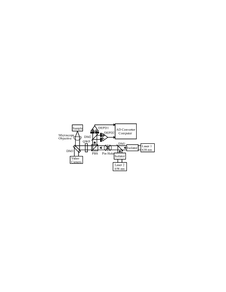
Figure 1: Experimental setup: Two independent laser beams are shone on the sample and their reflections are detected by dual-element photodiodes, DEPD1,2. A DEPD measures the inclination of the surface through the difference in the light intensities. A polarizing beam splitter (PBS) and a quarter wave plate (QWP) are included to extract the light reflected back from the sample efficiently. Dichroic mirrors (DM1,2) are used to combine or separate the light with the two different wavelengths. The data is processed by a computer via an analog-to-digital (AD) converter.

The experimental setup is shown schematically in Fig. 1. In our spectral measurements using surface light scattering, the average inclination of the surface within the beam spot is measured by using the difference between the reflection signals from two adjacent photodiodes. Since we need two independent measurements to obtain the signal as in Eq. (1), we use two sets of two photodiodes, DEPD1,2. Laser diodes with wavelengths 638 nm and 658 nm with a power 40 mW each were used as light sources. Due to the losses from stabilization, the power of the beam applied to the sample is 2 mW each, at most. When the sample is an organic matter, such as rubber, thermal effects from the beams are non–negligible so that a neutral density filter is used to further reduce the power of the beams. The most significant experimental limitations to the sensitivity in the measurement are various sources of cross-talk. This makes the experimental realization non-trivial, even though the principle explained above is simple. Cross-talk can arise from such diverse sources as the the AD converter, non-linear elements in the optical elements and coupling through the electromagnetic fields. In our experiments, we measured the size of the cross-talk prior to the measurements and corrected for it.

The major causes of noise in the experiment are the shot noise and the thermal noise in the detectors, often called Nyquist noise. These types of noise exist even in ideal experimental situations. Our method, as explained above, can suppress both types of noise and measurements can be made at orders of magnitude below the noise level, as explicitly demonstrated below. The thermal noise level in the detectors is mostly much less than the shot noise level and at most, of the same order in our experiments. Thermal noise can also be reduced, at least in principle, by cooling the detector while such methods are not applicable for the shot noise, which is essentially quantum in nature. The main error in our work is the theoretical limitation due to the number of averagings, $\cal N$. In theory, as well as in practice, this places a limitation that if a frequency resolution $\Delta f$ is required, time ${\cal N}/\Delta f$ is necessary to make the measurement. In our experiments, the time used for the measurements varied from 30 seconds to 30 minutes, longer times being used for weaker signals. One might point out that to overcome the error due to the shot noise, one can consider raising the power of the signal by increasing the light beam power. However, this is not always possible since raising the power can affect the sample itself, making it impossible to obtain meaningful results. Furthermore, large power is prohibitive in situations where non–invasiveness is required, such as medical applications. Given the same power, our method, when applicable, can extract far weaker signals than those obtainable by other methods.

We first observe and analyze thermal fluctuations on simple liquid surfaces. Thermal fluctuations of surfaces appear as capillary waves called “ripplons” and light scattering from them have been studied for some timeripplon ; ripplonExp . The dispersion relation of ripplons for a simple liquid has been derived theoretically, including its magnitude asLevich ; Bouchiat

$$P_{\rm R}(q,\omega)={k_{\rm B}T\over\pi\omega}{q\tau_{0}^{2}\over\rho}{\rm\,Im}\left[(1+s)^{2}+y-\sqrt{1+2s}\right]^{-1}$$ (2)

Here, $s\equiv-i\omega\tau_{0}$, $\tau_{0}\equiv\rho/(2\eta q^{2})$, $y\equiv\sigma\rho/(4\eta^{2}q)$. $\rho,\sigma,\eta$ are the density, the surface tension and the viscosity of the liquid. $q,\omega$ are the wave number and the frequency of the capillary waves. $k_{\rm B}$ is the Boltzmann constant and $T$ is the temperature. Our method differs from previous surface light scattering measurements in that we directly measure the spectrum of surface inclination fluctuations. Our observations correspond to the spectrum

$$S_{\rm R}(\omega)=\int\!\!\!{d^{2}q\over(2\pi)^{2}}\,q^{2}e^{-b^{2}q^{2}/8}P_{\rm R}(q,\omega)\qquad.$$ (3)

Here, $b$ is the diameter of the gaussian beam and the $q^{2}$ factor arises from observing inclinations. The vertical displacement spectrum is $b^{2}S_{\rm R}(\omega)$ so that the measured spectral density in these fluctuations go down to $\sim 10^{-29}\rm\,m^{2}$/Hz. When integrated over all frequencies, the total vertical displacement is few angstroms.

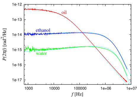
Figure 2: (Color online) Power spectrum of capillary waves on water(green), ethanol(blue) and oil surfaces(red). The theoretical predictions for them are also indicated (cyan) which agree quite well.

The theoretical results Eq. (3) agree quite well with the experimental observations, as shown in Fig. 2. The properties of the liquids are $(\rho\,{\rm[kg/m^{3}]},\sigma\,{\rm[kg/s^{-2}]},\eta\,{\rm[kg\cdot m^{-1}s^{-1}]})=(1.0\times 10^{3},7.3\times 10^{-2},1.0\times 10^{-3})$, $(0.79\times 10^{3},2.2\times 10^{-2},1.1\times 10^{-3})$, $(0.92\times 10^{3},3.0\times 10^{-2},0.124)$ for water, ethanol and immersion oil. The beam diameters are $b=2.5\,\mu$m for oil, ethanol and $3.2\,\mu$m for water. In Fig. 2, the overall magnitude of the signal was adjusted to fit the theoretical formula. This magnitude was independently calibrated using a pizoelectrically driven mirror and was confirmed to within a factor of two. Due to the relatively high viscosity of oil, there is a qualitative difference for the oil surface spectrum which decays as $f^{-2}$ for higher frequencies, when compared to those of water and ethanol which decay as $f^{-4}$. This is well reproduced in the measurements.

The shot noise level in our measurements is independent of $f$ and can be estimated as $N_{\rm SN}(\omega)={N\!A^{2}e/(2I)}$, where $I$ is the photocurrent, $N\!A$ is the numerical aperture of the objective lens and $e$ is the electron charge. We used a lens with $N\!A=0.5$ throughout and the photocurrent in all our measurements is $0.1$ to few $\mu$A. The ambient temperature was 25^∘ C for all our measurements. $N_{\rm SN}\simeq 2\times 10^{-15}\,\rm[rad^{2}/{\rm Hz}]$ in the above ripplon measurements so that the measurements in Fig. 2 go down to a couple of orders of magnitude below the shot noise level.

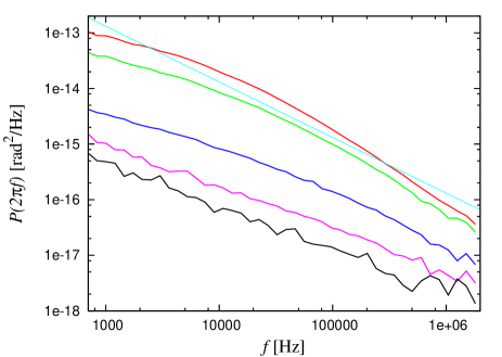
Figure 3: (Color online) Power spectrum of surface fluctuations of rubber in the elongated direction, when the extension ratio is 1 (red),2 (green), 3(blue), 4 (magenta), 6 (black). The fluctuations decrease under stretching. For comparison, the theoretical formula corresponding to surface fluctuations of an elastic material is also shown (cyan). $N_{\rm SN}\simeq 1\times 10^{-14}\rm\,[rad^{2}/Hz]$ in this measurement.

Using the same method, the surface fluctuations of rubber with varying strain are observed in Fig. 3. An estimate for the fluctuation spectrum as an elastic mediumSaulson90 ; Levin ; Braginsky99 is

$$S_{\rm S}(\omega)={16k_{\rm B}T\over\sqrt{\pi}\omega b^{3}}{(1-\sigma_{\rm P}^{2})\phi\over Y}\qquad.$$ (4)

Here, $Y,\sigma_{\rm P},\phi$ are the Young’s modulus, Poisson’s ratio and the loss angle of the material. In the plot, we used natural rubber stretched to various lengths. As a guide, we indicated the spectrum in Eq. (4) with frequency independent $Y=3.5\times 10^{6}\,\rm[kg/(m\cdot s^{2})],\sigma_{P}=0.475,\phi=0.1$, which are typical values for rubber. The dependence on $f$ does not agree completely with this idealized material, which is natural since $Y,\phi$ depend on $f$rubber and rubber is a complex material that changes its state as it is elongatedrubberStretch . Obviously, the dependence can be perfectly reproduced if we assume a particular $f$ dependence for $\phi/Y$. The signal decreases as the Young’s modulus increases when the rubber is stretchedrubberStretch . We have also measured the fluctuations in the inclinations transverse to the direction of extension and find them to be larger than those parallel to it, as expected, indicating the existence of more flexibility in the transverse direction. The laser beam used had a diameter $1\,\mu$m with a power 150 $\mu$W. Lowering this power did not change the spectrum. On the other hand, if the power is raised substantially, the beam affects the spectrum, presumably by heating up and perhaps melting the material. Consequently, this result is difficult to obtain without separating out the random noise using the logic explained in Eq. (1).

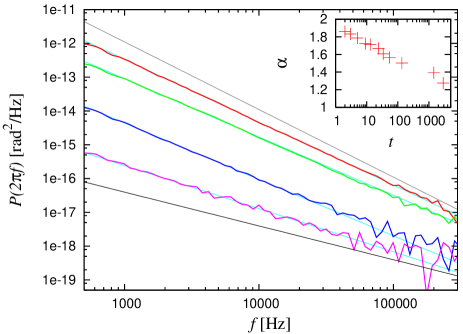
Figure 4: (Color online) Epoxy adhesive surface fluctuations 2 (red), 9 (green), 24 (blue) minutes and 2 days (magenta) after application, together with fits to them to functions of the form const.$\times f^{-\alpha}$ (cyan), which work quite well. As a guide, theoretical results for a simple liquid (grey) and an elastic material (black) are shown also. The fluctuations decrease with time. The change in $f$ dependence of the surface fluctuation power spectrum with respect to time $t$ [min] shows a slow decrease between $\alpha=2$ and $\alpha=1$ (inset). $N_{\rm SN}\simeq 4\times 10^{-15}\rm\,[rad^{2}/Hz]$ in this measurement.

We now consider a more complex material, an epoxy adhesive, whose properties change over time, as the glue “hardens”. Our method allows us to obtain spectral properties quickly without any contact and we can see how the spectrum changes with time. The measurements are shown in Fig. 4 where we used a laser beam a diameter of $1\,\mu$m. The thermal fluctuation spectrum at each instant can be well described by a simple power dependence $P(f)\sim f^{-\alpha}$. This power $\alpha$ slowly decreases with time with values between two and one, as in Fig. 4 (inset). We recall that for highly viscous fluids, $\alpha=2$ in this frequency range, as can be seen in Fig. 2, and $\alpha=1$ for elastic materials, as in Eq. (4). The results are quite consistent with an evolution of the epoxy adhesive between these two states. For comparison, the ripplon spectrum in Eq. (3) with typical values for an epoxy adhesive, $(\rho\,{\rm[kg/m^{3}]},\sigma\,{\rm[kg/s^{-2}]},\eta\,{\rm[kg\cdot m^{-1}s^{-1}]})=(1.5\times 10^{3},4.0\times 10^{-2},5000)$ and the spectrum for an elastic material with $(1-\sigma_{\rm P})^{2}Y/\phi=1.5\times 10^{11}\rm\,[kg/(m\cdot s^{2})]$ are also indicated. Phenomenologically, the time dependence of $\alpha$ can be well described by a logarithmic one in the relevant region (see Fig. 4 inset). The reason $\alpha$ decreases with time in such manner is worth further study.

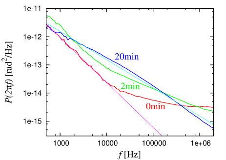
Figure 5: (Color online) Surface fluctuations of an ayu eye when it is wet (red) and 2 (green), 20 (blue) minutes thereafter. $6.0\times 10^{-8}f^{-1.6}$ is shown (magenta). Theoretical formula for an elastic material is also indicated (cyan). $N_{\rm SN}\simeq 2\times 10^{-14}\rm\,[rad^{2}/Hz]$ in this measurement.

Our method is well suited to biological materials since low power laser beams can be used. Fig. 5 shows the measurements of the surface fluctuation spectrum of an ayu (sweetfish) eye as it dehydrates. The laser beam in the measurement has a power of 200 $\mu$W and a diameter $1\,\mu$m. Measurements were performed when the eye was wet and then after certain time had passed. Not only quantitative, but clear qualitative differences in the fluctuation spectrum can be seen with time. At the beginning, the eye surface is wet and at lower frequencies, $f\lesssim 40$ kHz, the fluctuations decay as $\sim f^{-1.6}$ as can be confirmed in Fig. 5. This property is similar to that of a highly viscous liquid like oil in Fig. 2 and viscous complex fluid like epoxy in Fig. 4. For higher frequencies, $f\gtrsim 40$ kHz, the spectrum has almost no frequency dependence and behaves similarly to the water spectrum in Fig. 2, including its magnitude. This suggests that the material contains water substantially and is a gel like material. With time, water evaporates and the thermal fluctuation spectrum changes from that of a fluid to that of a solid. We show the surface fluctuations of an elastic material in Eq. (4) with $(1-\sigma_{\rm P})^{2}Y/\phi=4.0\times 10^{6}\,\rm[kg/(m\cdot s^{2})]$ in Fig. 5, which describes the spectrum after 20 minutes quite well. This spectrum is similar to the rubber surface fluctuation spectrum in Fig. 3.

In this work, we used an optical leveropticalLever to measure power spectra of thermal fluctuations of a wide variety of surfaces, from simple liquids to biological matter. By analyzing the fluctuation spectra of various types of matter and relating their spectra to their physical properties, the fluctuation spectra of complex materials could be qualitatively explained from the understanding of the spectra of simpler matter. The reason it is possible to make these sensitive measurements at our low optical intensity is because the measurements were performed down to orders of magnitude below the shot noise level. There are situations, such as gravitational wave measurements, which are usually believed to be shot noise limitedGS95 ; gravWaveExp and our method can perhaps significantly improve the capabilities of those. The measurements can be non–invasive and is applicable to all kinds of surfaces, including biological matter and may be effective in studying biological phenomena, such as the dry eye syndrome. Our measurement requires relatively a short time, allowing us to take spectral snapshots of surfaces, observing the time evolution of physical properties, as exemplified above.

References

- (1) M. von Schmoluchowski, Ann Physik 25, 225 (1908); L. Mandelstam, Ann. Physik 41, 609 (1913).
- (2) D. Langevin, “Light scattering by liquid surfaces and complementary techniques”, Marcel Dekker, New York (1992).
- (3) K. Numata et al, Phys. Rev. Lett. 91, 260602 (2003); E.D. Black et al, Phys. Lett. A 328, 1 (2004)
- (4) W. Denk and W. W. Webb, Appl. Opt. 29, 2382 (1990)
- (5) V.G. Levich, “Physicochemical Hydrodynamics”, Prentice-Hall, Englewood Cliffs (1962)
- (6) M.-A. Bouchiat, and J. Meunier, J. de Phys. 32, 561 (1971).
- (7) P.R. Saulson, Phys. Rev. D42, 2437 (1990)
- (8) Y. Levin, Phys. Rev. D57, 659 (1998)
- (9) V.B. Braginsky, M.L. Gorodetsky, S.P. Vyatchanin, Phys. Lett. A264, 1 (1999)
- (10) W. Philippoff, J. Brodnyan, J. Appl. Phys, 26, 846 (1955)
- (11) L.R.G Treloar, “The physics of rubber elasticity”, Oxford University Press, Oxford (2005)
- (12) T. Mitsui, Jpn. J. Appl. Phys., 47, 6563 (2008)
- (13) P. Fritschel et al, Phys. Rev. Lett. 80, 8181 (1998)
- (14) G.I.González, P.R.Saulson, Phys. Lett. A201, 12 (1995)