Mesoscopic conductance fluctuations in YBa₂Cu₃O_7-δ grain boundary Junction at low temperature

Abstract

The magneto-conductance in YBCO grain boundary Josephson junctions, displays fluctuations at low temperatures of mesoscopic origin. The morphology of the junction suggests that transport occurs in narrow channels across the grain boundary line, with a large Thouless energy. Nevertheless the measured fluctuation amplitude decreases quite slowly when increasing the voltage up to values about twenty times the Thouless energy, of the order of the nominal superconducting gap. Our findings show the coexistence of supercurrent and quasiparticle current in the junction conduction even at high nonequilibrium conditions. Model calculations confirm the reduced role of quasiparticle relaxation at temperatures up to 3 Kelvin.

I Introduction

In high critical Temperature Superconductor (HTS) junctions, including grain boundary (GB) structures, it is well established that various interplaying mechanisms contribute to transport with different weights still to be completely defined in a general and consistent framework Tsuei and Kirtley (2000); Hilgenkamp and Mannhart (2002); Tafuri and Kirtley (2005). As in all non-homogeneous systems, the barrier region will significantly contribute to determine the transport properties across the structure. What is peculiar of HTS is the complicate material science entering in the formation of the physical barrier microstructure. This will depend on the type of device and the fabrication procedure. The material science complexity of HTS may also result in different precipitates and inclusions present at interfaces and grain boundaries, and in some type of inherent lack of uniformity of the barriers Hilgenkamp and Mannhart (2002). All this has turned into some uncertainty about the nature of the barrier and has originated various hypotheses on the transport properties. The most wide-spread models are basically all in-between two extreme ideas Gross et al. (1997); Gross and Mayer (1991); Halbritter (1993, 2003); Moeckly et al. (1993); Sarnelli et al. (1994); Hilgenkamp and Mannhart (2002): on the one hand resonant tunnelling through some kind of dielectric barrier Gross et al. (1997); Gross and Mayer (1991); Halbritter (1993, 2003), on the other, especially in GB junctions, a barrier composed of thick insulating regions separated by conducting channels, which act as shorts or microbridges Moeckly et al. (1993); Sarnelli et al. (1994). In most cases the interface can be modeled as an intermediate situation between the two limits mentioned above. A transition from one extreme to the other can therefore take place. What is unfortunately missing is a way to describe this tuning-transition through reliable and well defined barrier parameters (for instance the barrier transparency). The predominant d-wave order parameter symmetry (OPS) is another important Tsuei and Kirtley (2000), to which a large part of the phenomenology has been clearly associated Tsuei and Kirtley (2000); Hilgenkamp and Mannhart (2002); Tafuri and Kirtley (2005); Lofwander et al. (2001); Kashiwaya and Tanaka (2000). D-wave OPS implies the presence of antinodal (high energy), and nodal (low energy) quasi-particles in the conduction across junctions and the absence of sharp gap features in the density of states of the weak link. Recently, low temperatures measurements have proved macroscopic quantum tunneling (MQT) in YBCO GB junctions, stimulating novel research on coherence and dissipation in such complex systems Lombardi et al. (2002); Bauch et al. (2006); Bauch and et al. (2005).

In this work we report on an investigation of magnetoconductance at low temperatures for the same type of biepitaxial GB junctions Tafuri et al. (1999), used for the MQT experiments. These structures are very flexible and versatile, guaranteeing on the one hand low dissipationBauch et al. (2006); Bauch and et al. (2005) and on the other a reliable way to pass from tunnel-like to diffusive transport on the same chip by changing the interface orientationLombardi et al. (2002); Tafuri et al. (1999). We give direct evidence of the role played by narrow conduction channels across the GB. These channels may have different sizes and distributions and obviously a different impact on the transport properties. When increasing applied voltage, mesoscopic conductance fluctuationsB.L.Altshuler and A.G.Aronov (1985); Lee and Ramakrishnan (1985); Lee and Stone (1985); Lee et al. (1987); Altshuler and Lee (1988) appear in our samples, at low temperatures, not dissimilar from what is usually observed in normal narrow metal samples Pierre et al. (2003). We expect that, in our sample, typical sizes of the current-carrying constrictions $L_{x}$ and $L_{y}$ range from 50 nm to 100 nm and, as a consequence, Thouless energy $E_{c}$ ( see Table 1 ) turns out to be quite large, when compared to the values usually measured in traditional normal metal artificial systems van Oudenaarden et al. (1997). The mesoscopic effects persist at voltages about twenty times larger than the Thouless energy. ”Novel” mesoscopic issues that emerge from the analyses carried out in the present work are tightly connected to the nature of the GB systems: a) a smooth crossover appears to exist from the coherent conduction mostly driven by the supercurrent, to the magnetoconductance driven by quantum coherent diffusion of quasiparticles across the mesoscopic area, when the voltage at the junction increases; b) in analogy to pairs, quasiparticles also appear to have a large phase coherence as proved by the shape of the power spectrum of the conductance fluctuations, up to temperatures of 3K; c) the voltage drop appears to be concentrated at the GB, and non equilibrium does not affect substantially the mesoscopic interference over a wide area about $1\mu m^{2}$.

This work builds upon a previous report, where the main ideas have been illustrated Tagliacozzo et al. (2007). Herein a more complete analysis of the experimental data is carried out. We have applied the ”protocol” established in the last 20 years on semiconducting and normal metal nanostructures to our system and we have extracted the characteristic lengths and scaling energies.

In Section II we give some details about the sample fabrication. By presenting the magnetic mesoscopic fingerprints of our sample in Section IIIA, we collect evidences of the mesoscopic character of the conductance fluctuations that we have measured. In section IIIB we derive from the ensamble average of the fluctuations the variance of the conductance, which is presented in section IIIC.

In Section IV we show the conductance autocorrelation for different magnetic fields in an intermediate voltage range. By analyzing the power spectral density we estimate the phase coherence length $L_{\varphi}$ which is found to be $\lesssim L$, at intermediate voltages ( $V=14\div 18$ mV). The conductance autocorrelation at different voltages allows us to interpret the role of nonequilibrium by defining the voltage dependence of the phase coherence length, as discussed in Section V. The discussion of the results can be found in Section VI. Our simple model theory well accounts for the experimental results and clarifies the survival of non locality in the quantum diffusion in presence of a large voltage bias. Table 1 gives additional information on the planning of this work. Our conclusions can be found in Section VII.

Table 1: Summary of the results:

Topic	Relative measurement	Extracted parameters	Estimates
Junction geometry	Magnetic pattern: $I_{C}\>vs.\>H$ in Fig.(3)	$L_{x}\sim L_{y}\sim 50nm$	$E_{c}\sim 1mV$
Transport properties	$R_{N}$ in Fig.(4) and $I_{c}R_{N}$ in Fig.(2)	$R_{N}=400\Omega$, $T\gtrsim 257mK$	$I_{c}R_{N}\sim E_{c}/e$
Mesoscopic Fingerprints	Resistance fluctuations in Fig.s(5,6)	$var[g]\lesssim 1$
Phase coherence length	Autocorrelation vs $\Delta H$ in Fig.(7), PSD in Fig.s(8,9)	$L_{\varphi}\lesssim 1\mu m$	$L_{\varphi}\sim V^{-1/4}$
Coherent phase breaking time	Autocorrelation vs $\Delta V$ in Fig.(10)	$\tau_{\varphi}\sim 400\>ps$	$D\tau_{\varphi}\sim L_{\varphi}^{2}$

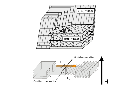
Figure 1: a) Sketch of the YBCO biepitaxial GB junction used in this experiment. b)Geometry of the model system of the current-carrying constriction.

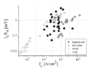
Figure 2: (color online) The product $I_{c}R_{N}$ is reported as a function of the critical current density $J_{c}$. Data are collected from Ref.s Hilgenkamp and Mannhart (2002); Tafuri and Kirtley (2005); Dimos et al. (1990); Hilgenkamp and Mannhart (1998); Ivanov et al. (1991); Char et al. (1991)

II fabrication and average transport properties of the sample

The $GB$ Josephson junctions are obtained at the interface between a (103)YBa₂Cu₃ O_7-δ ($YBCO$) film grown on a (110) SrTiO₃ substrate and a $c$-axis film deposited on a (110) CeO₂ seed layer (see Fig.(1)). The presence of the CeO₂ produces an additional 45^∘ in-plane rotation of the $YBCO$ axes with respect to the in-plane directions of the substrate Lombardi et al. (2002). The angle $\theta$ of the grain boundary relative to the substrate $a,b$ axes is defined by suitably patterning lithographically the CeO₂ seed layer (see Fig. (1 a)). Details about the fabrication process and a wide characterization of superconducting properties can be found elsewhere Tafuri et al. (1999); Lombardi et al. (2002). The interface orientation can be tuned to some appropriate transport regime, evaluated through the normal state resistance $R_{N}$ and critical current density (J_C). Typical values are reported in Fig.(2) and compared with data available in literature Tafuri and Kirtley (2005).

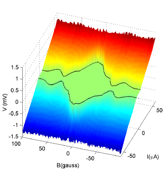
Figure 3: (color online) The I-V characteristics as a function of magnetic field.

In the tilt cases J_C $\approx$ 10³ A/cm² and $\sigma$_N=$1/(R_{N}A)$ $\approx$ 0.2(m$\Omega$cm²)^-1, both measured at T = 4.2 K (A is the junction cross section). Twist GBs junctions are typically characterized by higher values of J_C in the range 0.1-4.0 x 10⁵ A/cm² and $\sigma_{N}\approx$10 (m$\Omega$cm²)^-1 (at T = 4.2 K).

We have selected YBCO grain boundary junctions and measured their I-V curves at low temperatures T, as a function of the magnetic field H applied in the direction orthogonal to the plane of the junction. In HTS junctions, the correlation between the magnetic pattern and the current distribution profile along the junction is made more complicate by the d-wave order parameter symmetry (OPS), which generates anomalous magnetic response especially for faceted interfacesTsuei and Kirtley (2000); Hilgenkamp and Mannhart (2002); Tafuri and Kirtley (2005); Mannhart et al. (1996). Additional deviations are expected because of the presence of the second harmonic in the current-phase relation Lofwander et al. (2001); Kashiwaya and Tanaka (2000). In Fig.(3) we report the magnetic field dependence of the IV characteristics of the maximum Josephson current of the of the junction that we have extensively investigated in this work (with barrier orientation $\theta$=60^∘). This angle gives the maximum $J_{C}$Lombardi et al. (2002). The magnetic response presents a maximum of the critical current at zero field and two almost symmetric lobes for negative and positive magnetic fields respectively. At higher magnetic fields (above 100 G or below -100 G), the critical current is negligible. The flux periodicity is roughly consistent with the size we expect for our microbridge (50-100 nm), since the London penetration depth in the off-axis electrode is larger than the one in c-axis YBCO films, of the order of microns (see Ref. Bauch and et al. (2005) and Tafuri and Kirtley (2000) for instance). Experimental data can be compared with the ideal Fraunhofer case in the crudest approximation without taking into account the presence of a second harmonic or any specific feature of HTS. Even if deviations from the ideal Fraunhofer pattern are present, they can be considered to some extent minor if compared with most of the data on HTS grain boundary Josephson junctions, which present radical differences. We can infer an uniformity of the junction properties approximately on an average scale of 20-30 nm, which is remarkable if compared with most results available in literature. Even if we cannot draw any conclusion on the current distribution on lower length scales, we can rule out the presence of impurities of large size along the width of the active microbridge. In fact, were there more than one active microbridge, the current of each of them would add in parallel and the pattern would present other periodicities referring to the area enclosed between the conduction channels (Ref.Barone and Paternò (1982)). The I-V characteristics of the HTS Josephson junctions still present features, which cannot be completely understood in terms of the classical approaches used to describe the low critical temperature superconductors Josephson junctions. These are frequently observed and often referred in literature as unconventional features Tsuei and Kirtley (2000); Hilgenkamp and Mannhart (2002); Tafuri and Kirtley (2005). Examples areTafuri and Kirtley (2005): a) I_CR_N values are much lower than the gap value $\Delta$; b) the shape of the I-V strongly depends on the critical current density; c) I-V curves show significant deviations from the Resistively Shunted Junction model (RSJ); d) there is a poor consistency between the amplitude of the hysteresis and the extracted values of the capacitance, when compared to low-$T_{C}$ superconductor junctions.

At low temperatures, the resistance vs applied current $R(I)$, as derived from the I-V characteristics is rather temperature insensitive, while the critical current $I_{C}$ maintains a sizable temperature dependence. In the inset of Fig.(4) we show the resistance $R(I)$ at zero magnetic field for three temperatures: $257mK$, $1K$ and $3K$. $R(I)$ obviously vanishes in the Josephson branch and displays a sharp peak when switching to/from the finite voltage conductance. The data are displayed in order to show the critical current at $I>0$ and the retrapping current at $I<0$. In Fig.(4,main-panel) we show a blow up of the resistance $R(V)$ in a range of voltage values $V$ between $0.25\>mV$ and $30\>mV$ at zero magnetic field and for different temperatures $T=257mK,1K,3K$.

Measurements have been taken after different cool-downs in the time lapse of two years to study the sample dependent properties.

The average resistance in the range of voltages $V\approx 10mV\div 15mV$ has been stable for about eighteen months at $\sim 180\>\Omega$ and has increased in the last year up to about $430\>\Omega$. These changes should be attributed to aging of the diffusion properties at the grain boundary. However, in the meantime, no significant change of the $I_{C}$ has been detected. Only one sample was available with such a reduced width. The steady progress in nanotechnology will probably lead to the realization of reliable microbridges of nominal width of a few hundred nanometers, from which it will be easier to have junctions with transport carried by very few mesoscopic channels. We finally signal a strong similarity of the I-V and dI/dV-V curves of our junctions with those from sub-micron YBaCuO junctions, reported in Ref.Herbstritt et al., 2001.

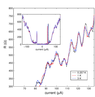
Figure 4: (color online) Main: zooming on the oscillations of $R\>vs.\>I$ above $I\approx 80\mu A$. Inset: Resistance as a function of applied bias current for three different temperatures: $257mK,1K,3K$.

III Magnetoresistance and mesoscopic fingerprints

III.1 Resistance fluctuations

According to what reported in the previous Section, we figure out that most of the current in the junction substantially flows across a single nanobridge of characteristic size $L_{x}<~{}$ 100nm. Possible lack of spatial uniformity of the current distribution on a scale of less than 20 nm does not affect the arguments developed below.

We call $x$ the flow direction and $y$ the direction perpendicular to the nanobridge, as shown in Fig.(1b). The diffusion coefficient $D$ in $YBCO$ is expected to be $\sim 20\div 24\>cm^{2}/sec$N.Gedik et al. (2003). By estimating the Fermi velocity $v_{F}\approx 7\times 10^{7}\>cm/sec$ for optimally doped $YBCO$, we conclude that the mean free path $\ell$ is smaller than the size of the nanobridge. Therefore we argue that the transport in the junction is diffusive, which is confirmed by the observation of the resistance fluctuations.

The Thouless energy, as derived from the expected size of the nanoconstriction, is $E_{c}=\hbar D/L^{2}\gtrsim 1\>meV$. This value is confirmed by our measurements as discussed in Section III. The number of transverse scattering channels in the constriction for a fixed cross section $A$ is approximately ${\cal{N}}_{ch}\approx k_{F}^{2}A\sim 5\cdot 10^{4}$. $A\sim 100\times 100\>nm^{2}$ is given by the product of the thickness of the film and the width of the channel. Hence, quantization of transverse levels in the bridge does not seem to play any role even at the lowest temperatures investigated. Indeed, $k_{B}T>>\delta\sim{E_{c}}/{\cal{N}}_{ch}\approx 0.1\mu eV$, where $\delta$ is the mean energy level spacing. As a consequence, our system can be thought as a disordered bridge in the diffusive limit $\ell<L_{x}$.

We concentrate on the marked non periodic fluctuations of the resistance at finite voltages, with magnetic field in the range $B=-100\div 100G$. An example of the magnetoresistance fluctuations is reported in Fig.(5) top panel for $T=257mK,1K,3K$.

The fluctuations are not related to the magnetic dependence of the Josephson critical current $I_{c}(H)$ at voltages $V>2mV$.

In order to avoid trapping of flux which may occur when increasing the temperature, especially at the higher fields, the data shown here refer to a single cool-down. Occasionally the pattern has still a slight deviation from reproducibility within one single cooling bath, which could be due to finite relaxation in the spin orientation of paramagnetic impurities. CONFERMARE The resistance pattern derived from our four terminal measurement does not show any mirror symmetry $R_{N}(H)\neq R_{N}(-H)$. Below 1K there is little temperature dependence. The amplitude of the fluctuations decreases between $T=1K$ and $T=3K$. They are sample dependent, as different cool-downs provide different patterns. All these features, as well as the ones described below, strengthen the conclusion that they are mesoscopic fluctuations.

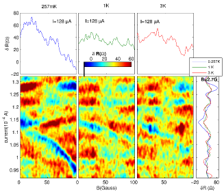
Figure 5: (color online) Color plot of the resistance fluctuations $\delta R(H,I)$ as a function of the applied current and of the magnetic field for three temperatures: $257mK$, $1K$, $3K$. The right panel shows $\delta R(H=2.7G,I)\>vs.\>I$ for the three different temperatures. The three top panels show single magnetoconductance trace for each temperature at fixed bias current (indicated in the labels).

The color plot of the resistance fluctuations in the $I,H$ plane provides the fingerprints of our sample. The deviation from the average $\delta R=R-\overline{R}$ is shown in Fig.(5) (three color-plot panels) as a color plot (color online), for three different temperatures, $257mK,1K,3K$. $\overline{R}$ is the average resistance performed over the full range of magnetic fields. The pattern keeps its shape within one single cool down and the contrast of the colors increases in lowering the temperature. The color scale is such that the dark red color refers to resistances significantly larger than the average, while the dark blue color refers to resistances significantly smaller then the average. The data have been filtered by gaussian convolution to get rid of the underlying white noise.

Despite the small equilibrium thermal length $L_{T}=\sqrt{\hbar D/k_{B}T}\sim 0.14\>\mu m$ at $1\>K$, there is a clear persistence of the fingerprints up to $T=3K$. This suggests that the strong non-equilibrium conditions induced by the applied voltage do not allow the thermalization of the carriers in the sample. Indeed, our results do not change qualitatively up to $1.5\>K$ , and transport can be classified as non equilibrium quantum diffusive because $L_{\varphi}\lesssim L_{x}$. Here $L_{\varphi}$ is the phase coherence length for carriers diffusing in the junction area and is $\lesssim 1\mu m$ (see Section IV).

III.2 Ensemble average

The variance $var[g]$ is the ensemble average of the amplitude squared of the conductance fluctuations, $\langle(\delta g)^{2}\rangle$, where $g=G/(2e^{2}/h)$ is the dimensionless conductance. We analyze the fluctuations of the conductance obtained by averaging over runs at different magnetic fields up to $100G$, at different voltages. Here we argue that this average can be taken as an acceptable ensemble average and provides a bona fide information about the variance $var[g]$ of the conductance and its autocorrelation. To justify our statement, we have to show that the Cooperon contribution to the variance is not significantly influenced by $H$ up to at least $100\>G$. The variance of the conductance at equilibrium at temperature $T$ can be calculated as Stone (1989)

$$var[g(H,T)]=\left.\frac{4s^{2}}{\pi^{4}}\int\frac{d\Delta E}{2k_{B}T}\>f\left[\frac{\Delta E}{2k_{B}T}\right]\>\left[F_{D}(\Delta E,H_{1},H_{2})+F_{C}(\Delta E,H_{1},H_{2})\right]\right|_{H_{1}=H_{2}=H}$$ (1)

where $s$ is the spin degeneracy, $f(x)=(x\>cothx-1)/sinh^{2}x$ and $F_{D,C}$ are the Diffuson and Cooperon autocorrelation functions, respectively. They can be rewritten in terms of the eigenvalues $\lambda_{\alpha}^{D,C}$ of the diffusion equationRammer (1998):

$$\left[-D\left(-i\vec{\nabla}+\frac{e}{\hbar c}\left(\vec{A}_{1}\pm\vec{A}_{2}\right)\right)^{2}+\frac{1}{\tau_{in}}-i\frac{\Delta E}{\hbar}\right]\>\psi_{\alpha}=\frac{\lambda_{\alpha}^{D,C}}{\tau}\>\psi_{\alpha}\>\>.$$ (2)

Here $D\tau=l^{2}/d\sim 4\cdot 10^{-12}cm^{2}$ (where $d$ is the effective dimensionality ) and $\tau_{in}$ is the inelastic relaxation time ($\tau_{in}>>\tau\sim 0.2\>psec$). $A_{1},A_{2}$ are the vector potentials ($H_{1}$ and $H_{2}$ the magnetic fields) influencing the outer and inner conductance loops respectively and the $+/-$ sign refers to the $C/D$ propagator respectively. We have:

$$F_{D,C}=L^{-4}(D\tau)^{2}\>\sum_{\alpha}\left[\frac{1}{\left|\lambda_{\alpha}^{D,C}\right|^{2}}+\frac{1}{2}\Re e\frac{1}{{\lambda_{\alpha}^{D,C}}^{2}}\right]\>\>.$$ (3)

At zero temperature only $\Delta E=0$ contributes to the integral in Eq.(1), so that the eigenvalues become real. In the evaluation of the variance, $H_{1}=H_{2}=H$ implies that the Diffuson eigenvalues become insensitive of the magnetic field. Instead, the Cooperon eigenvalues depend on $2H$ and can be written in analogy with the Landau levels energies. It follows that :

$$F_{C}(\Delta E=0,H)\sim\frac{3}{2}\>\sum_{n=0}^{n_{max}}\frac{1}{\left(n+\frac{1}{2}+\frac{1}{\omega_{H}\tau_{in}}\right)^{2}}\sim\frac{3\pi^{2}}{4}\>\left(1-\frac{H}{H_{o}}\right)\>\>,$$ (4)

where $\omega_{H}=4eHD/\hbar c$. Eq.(4) defines a decay threshold field of the Cooperon $H_{o}\sim\pi hc/(12eD\tau)$, which derives from the truncation of the sum over the orbital quantum number $n$ at $n_{max}\approx\hbar/m\omega_{c}l^{2}$ ($\omega_{c}=eH/mc$ is the cyclotron frequency). This limitation is required by quantum diffusion ($\langle r^{2}\rangle_{n_{max}}>l^{2}$). The large value of $n_{max}$, In our case ($\sim 10^{2}$ for $H<600\>G$), determines $H_{o}\gtrsim 2.5\>Tesla$ which is far beyond the field strengths that can be applied to our sample without trapping flux due to vortices. This confirms that averaging over the interval of $H$ values $H\in(-100\div 100\>G)$ is equivalent to a sample average, without introducing significant field dependencies. In the following the ensamble average will be denoted by the symbol $\langle...\rangle_{H}$. As it is shown in the next Section, the typical magnetic field scale that arises from the autocorrelation of the conductance is $\sim 10\>G$, much smaller than the interval over which the average is performed.

In the rest of the paper, we will generically denote the conductance autocorrelation, which is an extension of Eq.(1), by $K_{g}$. This quantity depends on many variables: $T,H\equiv(H_{1}+H_{2})/2,\Delta H\equiv H_{1}-H_{2},V\equiv(V_{1}+V_{2})/2,\Delta V\equiv V_{1}-V_{2}$. When no ambiguity arises, we have taken the liberty to list just the parameters relevant to the ongoing discussion, in order to simplify the notation.

III.3 Variance of the conductance and different voltage regimes

The conductance is derived from the $I/V$ characteristic. We have checked the behavior of the differential resistance, measured through a standard lock-in method, and we have found qualitatively similar results.

In Fig.(6) (upper panel ) we have reported the measured conductance fluctuations $\>vs\>$ voltage bias and magnetic field at the temperature $T=257mK$, in a grey scale plot. The plot shows two different regimes:

• Low voltages ( $V<3mV$), where fluctuations appear to be very high. Fluctuations in this range mostly arise from precursive switching of the current out of the zero voltage Josephson state. The analysis of this range of voltages is better discussed within the Macroscopic Quantum Tunneling dynamicsBauch et al. (2006); it requires full account of the superconductive correlations and is not addressed in this paper.

• Large voltages ($V>5mV$) . In this regime we observe some reproducible, non periodic and sample dependent fluctuations. The variance of the conductance $<(\delta g)^{2}>_{H}$, is plotted $vs$ voltage bias ( Fig. (6) bottom panel) for two temperatures. The scale for its magnitude is estimated according to $\delta R/R=\delta g/g\approx 0.01$ with $R=410\Omega(T=300mK)$. The variance $var[g]$ stabilizes around unity at $V\gtrsim 7mV$. As the voltage increases $V\gtrsim 18$ mV, the variance is increasingly reduced. However, small amplitude fluctuations seem to persist over a wide voltage range up to values which are by far larger than those in normal constrictions. Fluctuations survive up to voltages which are many times the Thouless energy.

Here we focus on the variance $var[g]$ and on the autocorrelation of the magnetoconductance as a function of voltage at low temperatures up to $V>>E_{c}/e\sim 1\>mV$. Our data can be interpreted on the basis of models for the quantum interference of carriers transported in the narrow diffusive channel across the GB line. The experimental findings are consistent with a large Thouless energy $E_{c}$ and quite long dephasing times $\tau_{\varphi}$. A comparison of the data with the results of our models seem to confirm that non equilibrium effects induced by the voltage bias $V$ are not the source of heavy energy relaxation of the carriers, even at voltages $V>>E_{c}/e$. A discussion about the voltage dependence of the variance of the conductance for large voltages can be found in the Section VI. In the next Section we analyze the conductance autocorrelation at finite voltage in some detail, to extract information about the phase coherence length $L_{\varphi}$ and the phase coherence breaking time $\tau_{\varphi}$.

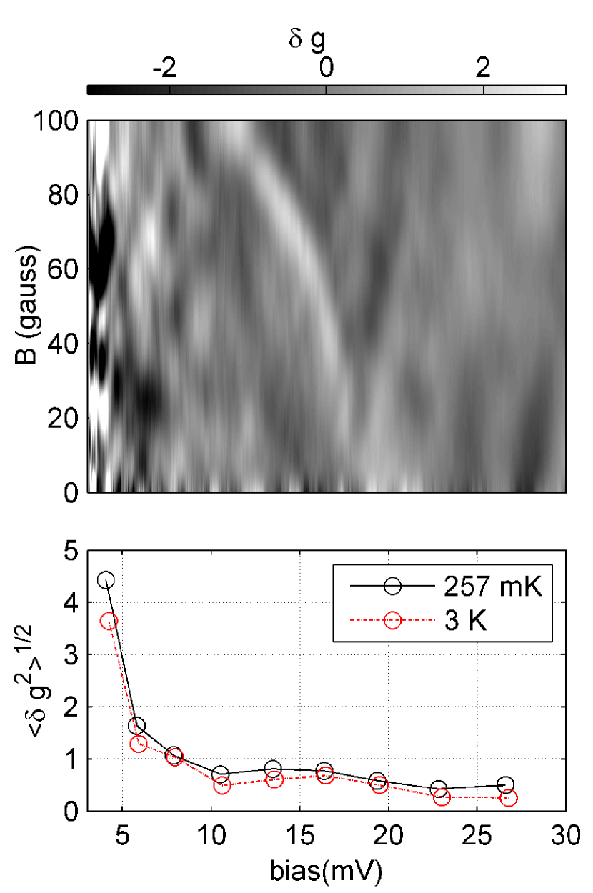
Figure 6: (color online)Top panel: grey-color plot of the fluctuations of the dimensionless conductance as a function of the voltage V and of the applied magnetic field H at $T=257mK$. Bottom panel: Variance of the dimensionless conductance as a function of the voltage V around zero magnetic field for T=257mK and T=3K.

IV Sampling nonlocality: autocorrelation $vs\;\;\Delta H$

The variance $var[g]$, of the conductance fluctuations $\langle(\delta g)^{2}\rangle_{H}$ discussed in Section III.C can be derived from the maximum at $\Delta H\approx 0$ of the more general autocorrelation function:

$$K_{g}(V,\Delta H)\equiv\langle\delta g(V,H+\Delta H)\delta g(V,H)\rangle_{H}$$ (5)

The data have been averaged over H, as usual, as well as over a small interval of voltage values about $V$. $K_{g}$ is the sum of Cooperon $F_{C}$ and Diffuson $F_{D}$ contributions. Due to the independence of our results of the temperature we consider the zero temperature limit of Eq. (1). In Fig.(7) we plot the measured autocorrelation of the dimensionless conductance vs. $\Delta H$ at $T=257mK$ for three values of $V$: $10\;mV$(blue curve), $14\;mV$ (red curve) and $18\;mV$ (red curve) (color online ). The data have been averaged over a voltage interval of width $\delta V=0.5mV$ (the results do not depend on this choice).

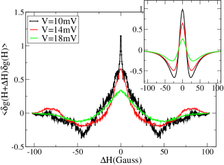
Figure 7: (color online) Autocorrelation $<(\delta g)^{2}>\;vs\;\Delta H$ at $T=257mK$ for three different values of the voltage drop: $V=10\>mV$ (black curve), $V=14\>mV$ (red curve), $V=18\>mV$ (green curve). Inset. Results of the model calculation sketched in the text for $\xi=1.05$ (black curve), $1.15$ (red curve), $1.4$ (green curve).

Similar curves have been measured for normal metal wires at zero voltage bias van Oudenaarden et al. (1997).

The autocorrelation of Fig.(7) is practically insensitive to increasing temperature up to about $1.5\>K$. This fact can be viewed as evidence that a significant contribution to transport and to the conductance fluctuations is still provided by the pair current. Its time average and absolute value can be seen as rather temperature and voltage independent, at fractions of Kelvin, while quasiparticles remain rather frozen, provided the voltage does not increase too muchbou . For weak links, characterized by and higher barrier transparency the contribution of the contribution of the supercurrent in the I-V curve can be relevant at finite voltagesLikharev (1979). The physical reason is that the phase changes in a sharply nonlinear manner with the greater part of the period being close to $\pi/2+2n\pi$. In addition, non-equilibrium effects Lehnert et al. (1999) and unconventional order parameter symmetry (with a not negligible second harmonic component in the current-phase Josephson relation A.A. Golubov (2004)) are possible additional sources of supercurrent flowing at finite voltage. Our results seem to confirm the presence of non negligible contribution of supercurrent at large voltages, from a different perspective. This is consistent with Ref.s Likharev, 1979; Lehnert et al., 1999; A.A. Golubov, 2004 and possibly with the observation of fractional Shapiro steps on YBCO grain boundary Josephson junctionsTerpstra et al. (1995); Early et al. (1993).

According to the remark made above, we can assume that the current at $T\sim 0$ is only a function of the phase difference $\varphi$ between the two superconducting contacts. This assumes little dephasing induced by inelastic scattering processes, but not necessarily the absence of quasiparticle contributions to the current which still depends on $\varphi$.

The inset of Fig.(7) shows the result of a simple model calculation of the autocorrelation function based on the following assumptions: $1)$ negligible proximity effect in the sub-micron bridge induced by the superconducting contacts; $2)$ an equilibrium approach to transport, in which the current is mostly phase dependent; $3)$ handling of the magnetic field $H$ is treated as a small correction and therefore $H$ only appears in the gauge invariant form of the phase difference.

The model (see Ref.Tagliacozzo and et al. (2008) for details) uses as unique fitting parameter $\xi=L_{y}/L_{\varphi}$, where $L_{y}$ is the transverse size of the conduction channel. The curves plotted in the inset are with $\xi=L_{y}/L_{\varphi}=$1.05 (black curve), 1.15 (red curve), 1.4 (green curve). The three different measured curves in the main plot of Fig.(7) refer to different bias voltages and cannot be directly compared to the theoretical curves in the inset of Fig.(7). The qualitative agreement between experimental and theoretical curves is evident, provided we assume that $\xi$ increases, with increasing voltage. This assumption is feasible since, on the one hand $L_{\varphi}$ is likely to be reduced when increasing applied voltage, and the number of conduction channels increases by changing the voltage and,as a consequence, the effective width of the bridge. If we assume that $L_{\varphi}$ scales with voltage as $V^{-1/4}$ ( see discussion in Section V ), we find that the $\xi$’s, that have been chosen to draw the inset of Fig.(7), are consistent with the voltages of the experimental curves within 15% of error.

The qualitative fit, based on the simple theoretical model used here, gives evidence of the fact that non-equilibrium does not seem to spoil the autocorrelation as a function of the magnetic field, even if the voltage bias exceeds the Thouless energy: $eV>E_{c}$. While the dephasing time $\tau_{\varphi}$ is discussed in the next Section, here we are in position to extract the value of the phase coherence length $L_{\varphi}$ from the Power Spectral Density (PSD) of the conductance autocorrelation function.

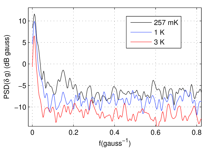
Figure 8: (color online) PSD at T= 257 mK, 1K, 3K and $V=7mV$, averaged over a voltage interval of $0.5mV$. The curves have been shifted for clarity.

The Power spectral density (PSD) of the conductance autocorrelation is plotted in Fig.(8) vs $f_{H}$, the conjugate variable to the magnetic field $\Delta H$ , for data at T = 273 mK, 1K, 3K and V= 7 mV. $f_{H}$ has the dimension of an inverse magnetic field. Inspection of Fig.(8) shows that there is a linear slope at small frequencies and a roughly flat trend at larger frequencies. The latter is due to the white noise affecting the measurement. Curves have been shifted, in the figure, for clarity. In reality, both the linear slope and the constant value are almost independent of the temperature. The linear slope allows to extract the value of the phase coherence length $L_{\varphi}$ according to the fitHohls et al. (2002):

$$log(PSD/PSD(f_{H}=0))=-2\pi f_{H}H_{c}+cnst\>\>,$$ (6)

as correlation field $H_{c}$ can be related to $L_{\varphi}$ as follows: $L_{\varphi}\sim\sqrt{hc/2eH_{c}}$. From this plot we derive $H_{c}\sim 10\>G$, that gives $L_{\varphi}\lesssim 1\>\mu m$.

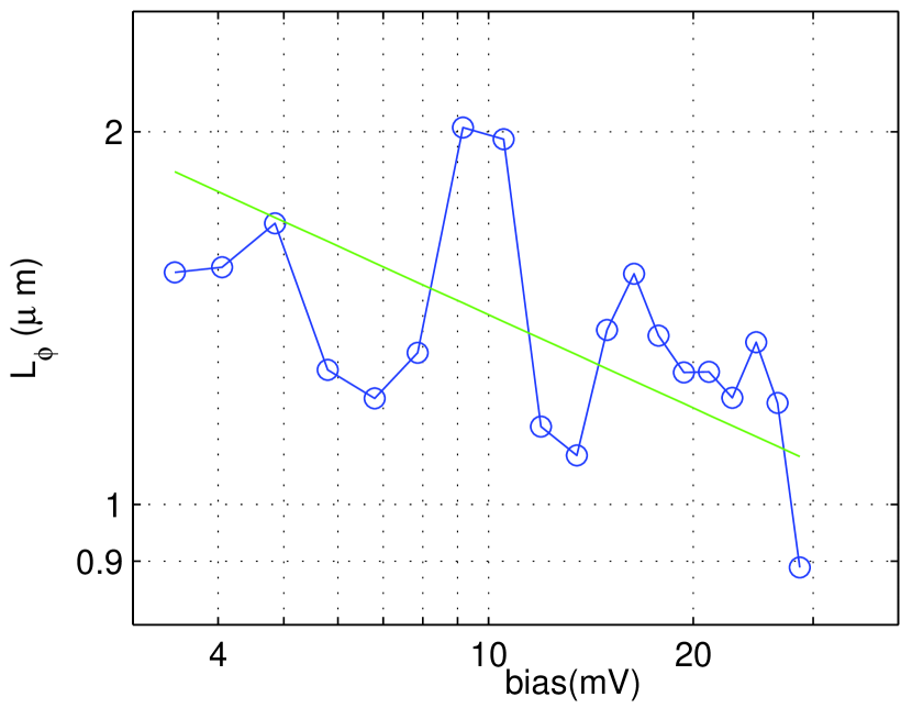
Figure 9: Logarithmic plot of $L_{\varphi}$ vs $V$ derived by using the eq.(6). Full lines are a guide to the eye. The slope of the straight line is $-1/4$.

A logarithmic plot of the $V$ dependence of $L_{\varphi}(V)$ is reported in fig(9). The straight line drawn among the experimental points shows the functional dependence $V^{-1/4}$.

V Non equilibrium effects on $\tau_{\varphi}$

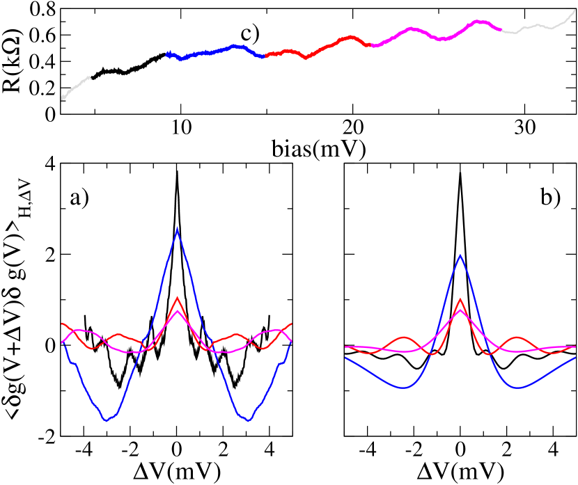
Figure 10: ( color online) The measured autocorrelation of the conductance $K_{g}(V,H=0,\Delta V)$ vs. the voltage difference $\Delta V$, for average voltages $V\approx 7.5,12.5,17.5,25.0\>mV$ ( panel $a)$); theoretical fit based on Eq.(10) (panel $b)$); Resistance $R\>vs.\>V$ (panel $c)$). There is correspondence between the colored ranges of panel $c)$ and the colors of the curves of the panels $a)$ and $b)$.

In this Section we study the dependence of the autocorrelation function on $V$ and $\Delta V$:

$$K_{g}(V,\Delta V)\equiv\langle\delta g(V+\Delta V,H)\delta g(V,H)\rangle_{H}\>.$$ (7)

A voltage average has been performed over intervals centered at $V$, of typical size lower than the $min\{E_{c},\Delta V\}$.

In Fig.(10$a$) we report the experimental autocorrelation function $K_{g}(V,\Delta V)$ vs $\Delta V$ for various values of the applied voltage $V$. We stress that the applied voltage is larger than the two natural energy scales: $E_{c}/e\sim 1\>mV$ and the nominal superconducting gap $\Delta/e\sim 20\>mV$. The tail of the curves shows a large anti-correlation dip when $\Delta V$ increases and damped oscillations. The autocorrelation maximum flattens when the applied voltage $V$ increases. Fig.(10 $c$) emphasizes the voltage range to which each curve of the panel $a$ refers, by using the same color.

We have reproduced the same trend of the data in Fig(10 $a$),by assuming that proximity effect induced by the superconducting contacts does not play an important role in the transport and by adapting the quasi- one-dimensional non-equilibrium theory of Ref.(A.I.Larkin and Khmel’nitskii, 1986; T.Ludwig et al., 2004) to our case (see Fig(10 $b$)). We will report on the derivation of our theoretical results elsewhereTagliacozzo and et al. (2008). We just mention that, our nonequilibrium approach gives rise to an autocorrelation $K_{g}(V,\Delta V)$ which is a function of $x=e\Delta VL^{2}/\hbar D$ and of the parameters $\tau_{\varphi}/\tau_{C/D}$ and $(L/L_{\varphi})^{3}$. Here $\tau_{C/D}^{-1}={e^{2}L_{y}^{2}D(H_{1}\pm H_{2})^{2}}/({12\hbar^{2}c^{2}})$ (with the + (-) sign for the C (D) case ) is the relaxation time induced by the magnetic field I.L.Aleiner and Ya.M.Blanter (2002). In the limit of vanishing $\Delta V$, the result for the variance is recovered, which, up to numerical factors, is given in terms of the ratio between the Airy function $Ai(u)$ and its derivative with respect to the argument $Ai^{\prime}(u)$:

$$K_{g}(V,\Delta V=0)=-{\left(\frac{D\tau_{\varphi}L_{\varphi}}{L^{3}}\right)}\>\sum_{\nu=C,D}\>\Re e\left\{\frac{Ai\left(\frac{2\tau_{\varphi}}{\tau_{\nu}}\right)}{\>Ai^{\prime}\left(\frac{2\tau_{\varphi}}{\tau_{\nu}}\right)}\right\}\>\>.$$ (8)

$\tau_{\varphi}$,$L_{\varphi}$ and $\tau_{\varphi}/\tau_{\nu}$ all depend on the voltage. This formula is similar to the thermal equilibrium result by Altshuler, Aronov, Khmielnitski (AAK)B.L.Altshuler et al. (1982), which includes the dephasing induced by e-e scattering with small energy transfer. In particular AAK find

$$\frac{1}{\tau_{\varphi}L_{\varphi}}=\frac{e^{2}k_{B}T}{\hbar^{2}\sigma}$$ (9)

where $\sigma$ is the conductivity. At intermediate applied voltages, our zero temperature prefactor $D\tau_{\varphi}L_{\varphi}/L^{3}$ in Eq.(8) looks similar to the AAK prefactor $\hbar DL_{\varphi}/(3\pi L^{3}k_{B}T)$ if $\hbar/\tau_{\varphi}$ replaces $k_{B}T$.

By choosing an appropriate voltage dependence of the fitting parameter ${\tau_{\varphi}}/{\tau_{\nu}}$ and $L_{\varphi}/L$, we find that the autocorrelation scales with $L_{\varphi}(V)$ as follows:

$$K_{g}(V,\Delta V)\approx\sum_{\nu=C,D}\>{\cal{F}}\left[\frac{\Delta V}{V_{c}},\frac{\tau_{\varphi}}{\tau_{\nu}},\left(\frac{L_{\varphi}}{L}\right)^{3}\right]\>\>\>,$$ (10)

with $D\tau_{\varphi}=L_{\varphi}^{2}$ and $\tau_{C}=\tau_{D}$, $V_{c}=\hbar/\tau_{\varphi}$. The explicit form of the function ${\cal{F}}$ will be given elsewhereTagliacozzo and et al. (2008). Its limiting form for $\Delta V\to 0$ gives Eq.(8). This scaling law is exploited to plot the curves of Fig(10b).

The scaling among the blue, red and cyan curves reproduces reasonably well the experimental pattern. This indicates that the $V$ dependence of eq.(10) is well accounted for by simply reducing $L_{\varphi}$ with increasing $V$. On the contrary, the black curve at the lowest voltage $V\sim 7.5mV$ requires adjusting the prefactor after the scaling, to make the central peak higher and narrower. This could be a hint to the fact that, when the voltage is rather low, the superconducting correlations may be relevant and should be included in deriving the functional form of the ${\cal{F}}$ function. Needless to say, an increase of the $\tau_{\varphi}/\tau_{\nu}$ parameter implies a reduction of the value of $var[g]$.

In writing Eq.(10), extra contributions arising from the non linear response have been neglected. Actually, Eq.(10) would be the result within linear response theory only, except for the $V$ dependence of $L_{\varphi}(V)$.

The global interpretation of the data given here shows that a monotonous decrease of $\tau_{\varphi}$ with increasing voltage is not achieved. A non monotonous decrease of $var[g]$ vs $V$ is indeed found, as can be seen from Fig.(6). According to the correspondence $D\tau_{\varphi}=L_{\varphi}^{2}$, and to Fig.(9) a general decreasing trend of $K_{g}(V,\Delta V)$ with increasing voltage could take over only above $20$ mV. In Eq.(8) derived from our model calculation, we have found $\hbar/\tau_{\varphi}$ in place of $k_{B}T$ appearing in the AAK result of Eq.(9). At larger voltages the expected substitution in Eq.(9) is T.Ludwig et al. (2004) $k_{B}T\to eVL_{\varphi}/L$ and, by requiring the consistency,

$$\frac{L_{\varphi}}{L}\sim\sqrt{\left.D\tau_{\varphi}\right|_{eVL_{\varphi}/L}}\>\>\>\to\left(\frac{L_{\varphi}}{L}\right)^{4}=\frac{D}{L^{2}}\>\frac{\hbar g}{eV}.$$ (11)

where $g=\hbar\sigma/(e^{2}L)$ in $1-d$. This would give a decay law for the coherence length $L_{\varphi}\sim V^{-1/4}$, which is not clearly recognizable in our experiment.

VI Discussion

We recollect here the main experimental facts that can be extracted from our data regarding quantum transport in a GB YBCO JJ .

The magnetic dependence of the maximum critical current suggests an active transport channel of the order of 50-100 nm. Uniformity of the critical current is on scales larger than about 20 nm. The Thouless energy $E_{c}=\hbar D/L^{2}$ turns out to be the relevant energy scale in this case. The normal resistance $R_{N}$ of the HTS junction is of the order of $200\Omega$, increasing up to $480\Omega$ with time, due to aging of the sample. The zero field Josephson critical current appears to satisfy $I_{C}R_{N}\sim E_{c}/e$. This product is definitely much smaller than $\Delta/e$, where the nominal superconducting gap is $\Delta=20\>meV$. This represents additional evidence that the proximity effect induced in the bridge in the absence of applied voltage is of mesoscopic origin. The superconductive pair coherence length $\xi_{s}<L_{\varphi}\lesssim L$, as opposed to the classical regime, $L<\xi_{s}$, when the tail of the order parameter enters both superconductors of the junctionP.Charlat et al. (1996). We speculate that the oscillations in the resistance as a function of $V$, shown in the inset of Fig.(4), could be due to this mesoscopic origin.

Remarkable conductance fluctuations have been found in a voltage range up to $20E_{c}$ in the magnetic field range of $H\in(-100,100)\>G$ for temperatures below 3 K. In the explored window, we do not measure an halving of the variance with increasing field $H$ J.S.Moon et al. (1997). The crossover field $H_{o}$ at which the Cooperon contribution to the variance is expected to disappear, as given by Eq.(4) is estimated of the order of few Teslas J.S.Moon et al. (1997). Decoherence induced by the Zeeman energy splitting requires even larger fields.

Transport has been measured in highly non-equilibrium conditions. Hence the temperature dependence is quite weak up to $T\sim 1.5\>K$. We have concentrated our analysis in the voltage range $V\in(7,30)\>mV$, where the conductance fluctuations reach a steady value for the variance at $T$ below 1 Kelvin, $var[g](V)\lesssim 1$. These properties confirm that the fluctuations are due to quantum coherence at a mesoscopic scale.

The PSD of the autocorrelation of the conductance at different fields $\Delta H$ allows to identify $H_{c}\approx 10\>G$ as the field scale for the mesoscopic correlations, weakly dependent on $V$. This value leads to a phase coherent length $L_{\varphi}\lesssim 1\>\mu m$. We have plotted the coherence length extracted from the autocorrelation PSD vs V in Fig.9 and compared it with $L_{\varphi}(V)\sim(V/V_{o})^{-s}$ with $s\sim 0.25$T.Ludwig et al. (2004). A similar exponent has been found in a limited range of voltage bias $V>E_{c}/e$ in gold samples Terrier et al. (2002), in which UCF (universal conductance fluctuations) and Aharonov-Bohm oscillations were found. Dephasing mechanisms are low frequency electron-electron interaction, magnetic impurity-mediated interactionKaminski and Glazman (2001) and non equilibrium quasiparticle distributionPothier et al. (1997). According to Fig.9, the comparison is not conclusive. As a matter of fact all data of conductance autocorrelation at finite voltage reported for normal wires van Oudenaarden et al. (1997); Terrier et al. (2002) identify a Thouless energy $E_{c}\sim 1\mu eV$, three orders of magnitude smaller than in our HTS device and refer to applied voltages not larger than $mV$’s. Still, mesoscopic coherence persists in our sample, up to voltages much larger than the Thouless energy. We do not find any linear increase of the conductance autocorrelation with voltage at large voltagesA.I.Larkin and Khmel’nitskii (1986).

Our model calculation appears to reproduce the gross features in the dependence of the conductance autocorrelation $K_{g}(V,\Delta H,\Delta V)$ on $\Delta H$ as well as on $\Delta V$. In the case of $K_{g}(V,\Delta H,0)$ we limit ourselves to the linear response term only and the effect of the voltage bias just appeared as a small reduction of $L_{\varphi}(V)$ with increasing $V$.

To model the trend of $K_{g}(V,0,\Delta V)$ vs $\Delta V$ given by the experiment, non-equilibrium cannot be ignored. Our derivation extends the calculation of Ref.(A.I.Larkin and Khmel’nitskii, 1986; T.Ludwig et al., 2004). We give a simple estimate of the conductance autocorrelation to fit our experiments. We invoke the simplest non-equilibrium distribution for diffusing quasiparticles, that is the collisionless limitPothier et al. (1997), by lumping the relaxation processes in the damping parameter of the Cooperon/Diffuson propagators $\tau_{C/D}$. The dependence on the applied voltage is introduced by tuning $\tau_{\varphi}$. We obtain oscillations in the negative tail of the autocorrelation, $K_{g}(V,0,\Delta V)$ (see Fig.(10)) and our scaling procedure fulfills the relation $D\tau_{\varphi}=L_{\varphi}^{2}$. Extra contributions that are specific of the non equilibrium theory and are known to be responsible first for a linear increase of the autocorrelation function with $V$ and subsequently for its power-law decay are not included here.

VII Conclusions

We have reported about transport measurements of high quality biepitaxial Grain Boundary YBCO Josephson Junction at temperatures below 1 Kelvin, performed over a time period of about 18 months. A global view on the data offers a consistent picture, pointing to transport across a single SNS(superconductor normal superconductor)-like diffusive conduction channel of mesoscopic size $L\lesssim 0.1\>\mu m$. We have mostly explored the magnetoconductance fluctuations in the voltage range $eV>>E_{c}>>k_{B}T$,where the Thouless energy $E_{c}\sim 1\>meV$. The Thouless energy, $2-3$ orders of magnitude larger than the one usually experienced in normal mesoscopic or low-$T_{c}$ superconducting samples, determines qualitatively the quantum coherent diffusion in the channel. We believe that the oscillations in the resistance that can be seen in Fig.(4) can be due to quantum diffusion.

The mesoscopic correlations are found to be quite robust in our GB narrow channel, even at large voltages. This could not occur if the lifetime of the carriers were strongly cut by non-equilibrium relaxation. We conclude that mesoscopic effects deeply involve superconducting electron-electron correlations, which persist at larger voltages. Transport features due supercurrents and quasiparticles at finite voltages cannot be disentangled in the pattern of the conductance, nor in its variance. This consideration has led us to approach the problem with a non-equilibrium model calculation for generic coherent transport, which highlights the role of the phase breaking time $\tau_{\varphi}$, without including superconducting correlation explicitly. Fig.10 shows the comparison between our model results and the autocorrelation experimental data, which is encouraging. The remarkably long lifetime of the carriers, which we find, appears to be a generic property in high-$T_{c}$ YBCO junctions as proved by optical measurementsN.Gedik et al. (2003) and Macroscopic Quantum TunnelingBauch et al. (2006).