The cluster birthline in M33

Abstract

Aims. The aim of this paper is twofold: $(a)$ to determine the reliability of infrared (IR) emission to trace star formation in individual star-forming sites of M33, and $(b)$ to outline a new method for testing the distribution function of massive stars in newly formed clusters.

Methods. We select 24 $\mu$m IR sources from the Spitzer survey of M33 with H$\alpha$ counterparts and show that the IR luminosities have a weak dependence on galactocentric radius. The IR and H$\alpha$ luminosities are not correlated. Complementing the infrared photometry with GALEX-UV data, we estimate the bolometric luminosities to investigate how they are related to the H$\alpha$ luminosities. We simulate a theoretical diagram for the expected bolometric-to-H$\alpha$ luminosity ratio, L_bol/L_Hα, of young clusters as a function of the cluster luminosity. We then compare the observed L_bol/L_Hα ratios with the theoretical predictions.

Results. In the log(L_bol)–log(L_bol/L_Hα) plane, stellar clusters should be born along a curve that we call the cluster birthline. The birthline depends on the stellar initial mass function (IMF) at the high-mass end, but not on the cluster mass function. For an upper stellar mass limit of $120\;M_{\odot}$, the birthline is flat for L${}_{bol}>3\times 10^{39}$ erg s^-1 because all clusters fully sample the IMF. It increases toward lower luminosities as the upper end of the IMF becomes incompletely sampled. Aging moves clusters above the birthline. The observations of M33 show that young isolated clusters lie close to the theoretical birthline for a wide range of L_bol. The observed L_bol/L_Hα ratio increases toward low L_bol like the theoretical curve, indicating that luminosity is not proportional to H$\alpha$ emission for low mass clusters. The best fit to the birthline is for a randomly sampled IMF, in which the mass of most massive star in a cluster is not strictly limited by the cluster’s mass, but can have any value up to the maximum stellar mass with a probability determined by the IMF. We also find that the IR luminosity of young stellar clusters in M33 is not proportional to their bolometric luminosity. This irregularity could be the result of low and patchy dust abundance. In M33 dust absorbs and re-radiates in the IR only part of the UV light from young clusters.

1 Introduction

Our knowledge of interstellar conditions that favor the birth of stars and clusters is mostly based on the Milky Way, but these studies are ill-suited for examining massive stars, which are an embedded population with a short lifetime. The number of Milky Way clusters that one can sample is also limited by extinction and distance uncertainties. These problems are somewhat diminished in studies of other galaxies, where imaging with high sensitivity and resolution is possible thanks to space observatories such as Spitzer, HST and GALEX. Soon we shall be able to know if the IMF and extinction in star-forming sites varies along the Hubble sequence, and if ISM perturbations from these sites vary with cluster position and mass. In the mean time, the best galaxies for study are in the Local Group. M33, at a distance $D=840$ kpc (Freedman et al. 1991), has a higher SFR per unit area than M31 (3.4 versus 0.74 M_⊙ Gyr^-1 pc^-2, Kennicutt 1998) and a lower extinction towards star-forming regions because of its lower inclination (e.g. Israel & Kennicutt 1980; Magrini et al. 2007b, and references therein). Bearing no prominent bulge and no signs of recent mergers, M33 is a prototype for star formation in a quiescent galaxy and for evolutionary scenarios in blue, low luminosity systems. Observations of the molecular, atomic and ionized gas in M33 have been carried out in the past years (e.g. Deul & van der Hulst 1987; Corbelli & Schneider 1997; Hoopes & Walterbos 2000; Corbelli 2003; Engargiola et al. 2003; Heyer et al. 2004). Together with recent works on the metallicity content of the young and old stellar population across the M33 disk, they allow us to trace the global formation and evolution history of the nearest blue disk galaxy (Magrini et al. 2007a, and references therein).

Verley et al. (2007, 2008) have shown that the recent Spitzer images of M33 allow us to study the average radial variation of star formation properties across the disk, and to locate stellar clusters and individual stars with infrared luminosities as low as $2\times 10^{37}$ erg s^-1 (corresponding to a B2 spectral type star on the main sequence). M33 therefore gives us a unique opportunity to study the properties of many individual star-forming sites, containing a range of populations from single O and B-type stars to young stellar clusters and associations. The observable luminosity range extends up to $(4.5\pm 1.5)\times 10^{7}\;L_{\odot}$ for NGC 604 (Israel et al. 1982, 1986; Hippelein et al. 2003), the second brightest HII complex in the Local Group.

The aim of this paper is to examine the conditions of the interstellar medium where stellar clusters are born, to define stellar cluster properties related to the birth and death of massive stars, and to examine star formation rate (SFR) diagnostics of individual complexes in M33. We will show the importance of complementing infrared photometry with photometry at optical and ultraviolet wavelengths. Previous papers outlined the need for infrared photometry to supplement H$\alpha$ in determining the SFR (e.g. Calzetti et al. 2005; Kennicutt et al. 2007, for M51). In bright star-forming regions of more distant and brighter galaxies, such as M51, there is a tight linear relation between IR luminosity and the strength of extinction-corrected, optical recombination lines (e.g. Calzetti et al. 2005). On the other hand, in late-type galaxies there are strong variations in the H$\alpha$-to-infrared flux ratio, which limits our ability to trace star formation via infrared photometry alone (e.g. Cannon et al. 2006, for the metal deficient Local dwarf NGC6822, where the H$\alpha$-to-IR flux ratio variations are as high as a factor 10). UV observations are also needed to trace the properties of star formation, particularly where the HII regions are density bounded or the O-type stars have evolved off the main sequence. GALEX observations of M33 have shown that the UV luminosity of a region is comparable to the IR luminosity (Verley et al. 2008), and is therefore a significant contribution to the total.

Here we employ a new technique to extract and measure sources from M33 images. Because dust and its associated IR emission are distributed in both star-forming complexes and the diffuse interstellar medium, we do photometry with varying apertures to match the source size at each wavelength. We also combine IR, UV and H$\alpha$ fluxes to give source properties down to very faint emission levels.

It is currently unknown if IR fluxes are good diagnostics for the SFR in areas where the bolometric luminosity of the newborn cluster is below 10⁴⁰ erg s^-1. M33 is an excellent candidate for studying individual low-mass clusters because its proximity minimizes contamination from the surrounding ISM. Whether low-mass clusters contribute substantially to the SFR of a galaxy depends on the initial cluster mass function (ICMF). In M33 the fragmentation process seems to favor small masses: the mass spectrum slope for giant molecular clouds (GMCs) is steeper than $-2$, as is the HII region luminosity function determined from H$\alpha$ emission (e.g. Wyder et al. 1997). Verley et al. (2007) have shown that the luminosity function at 24 $\mu$m can be described by a double power-law that is shallower than $-2$ at its faint end. While a change of slope like this could mark the transition between poor and rich clusters, occurring at the luminosity of the brightest star formed, a shallow slope at the low luminosity end can also indicate a decreasing dust abundance for lower masses. Giant complexes may form primarily in dust-rich environments, e.g. close to spiral arms, while low-mass clusters may form everywhere, also in low-dust environments. If some low-mass clusters are born in a low or patchy dust environment, then we cannot use IR luminosities alone to infer the SFR.

In this paper we will study the large scatter in the IR-to-H$\alpha$ ratio that is observed when young, low-luminosity stellar clusters are selected in M33. We show that complementing the IR photometry with UV photometry helps recover the total cluster luminosity and improves the correlation between stellar continuum and gas recombination lines from star-forming regions. We will examine in detail the theoretical and observed relation between L_bol and L_Hα, the deviations from the linear regime, and some properties of the massive stellar population in young clusters.

We shall also investigate the 8$\mu$m emission from PAHs in individual HII regions. Generally, PAH emission is low in dwarf and low-luminosity blue galaxies compared to other IR radiation. This may be related to the low metallicity and intense stellar radiation field in these systems relative to those in spiral galaxies (e.g. Galliano et al. 2003; Lu et al. 2003; Houck et al. 2004; Hogg et al. 2005; Rosenberg et al. 2006). Hunter et al. (2001) for example, used Infrared Space Observatory (ISO) mid-IR imaging and far-IR (FIR) spectroscopy to examine the properties of five dwarf irregular systems. They found that PAH emission, which is associated only with the brightest H II regions, is depressed relative to that of small grains and far-IR. In addition, the integrated [C II] emission relative to PAH emission is high in dwarfs compared to spiral galaxies, suggesting that atomic carbon is elevated relative to PAHs in dwarfs. Engelbracht et al. (2005) also examined low-metallicity systems and found that 8.0$\mu$m emission decreases abruptly relative to 24$\mu$m dust emission when the metallicity is less than one-third to one-fifth solar. M33 is a low-luminosity galaxy hosting HII regions with metallicities between solar and one-fifth solar and a shallow radial gradient (Magrini et al. 2007b; Rosolowsky & Simon 2008). PAHs are not globally underabundant in M33 although there is a faster decline of 8$\mu$m emission relative to longer wavelengths beyond 3.5 kpc (Verley et al. 2008). It is of interest then to examine possible metallicity and radial dependences of PAH features in individual HII regions.

In Section 2 we define young stellar cluster samples in M33 and analyze their IR properties. In Section 3 we study their UV luminosities and colors and define the cluster bolometric luminosities. The concept of cluster birthline is given in Section 4 and tested using M33 young clusters. In Section 4 we discuss the implications of our results relative to the dust abundance, to the bolometric to H$\alpha$ luminosity ratio, and to the population of massive stars in star-forming sites of M33. In the Appendix we analyze possible metallicity dependencies using a small sample of young clusters for which gas metal abundances are known, as well as dependencies of cluster properties on the mass of the associated giant molecular cloud.

2 Multiwavelength observations of star-forming sites

The closest star-forming galaxies offer a unique opportunity to resolve individual star-forming regions. In M33, the star formation process can be investigated not only by averaging over selected areas of the disk or by using very bright complexes, but also by observing individual star clusters of moderate size. The sensitivity of telescopes such as Spitzer in the IR and GALEX in the UV allows us to sample clusters over 4 orders of magnitude in brightness: from the second brightest HII region of the Local Group (NGC 604) down to clusters of about 1000 L_⊙. We can look in detail at the site properties where clusters of different masses are born, and at the emission properties of young clusters. We will use photometric information on sources across the M33 disk as given by the Spitzer 8$\mu$m and 24$\mu$m images described in Verley et al. (2007), by the GALEX FUV and NUV images from the GALEX Atlas (Gil de Paz et al. 2007), and by the H$\alpha$ image of Hoopes & Walterbos (2000).

2.1 The main sample

We define a sample of young stellar clusters and isolated massive stars using the IR catalog of 515 sources extracted from the 24$\mu$m Spitzer map by Verley et al. (2007). This catalog has a completeness limit of $3\times 10^{36}$ erg s^-1 (this limiting luminosity refers to the 90$\%$ level of completeness computed by extrapolation of the observed cumulative luminosity function at L${}_{24}>10^{37}$ erg s^-1). We remind the reader that the photometry for these sources has been done with a varying aperture to match the source size. From the catalog we select only sources that have an H$\alpha$ counterpart. We search for H$\alpha$ counterparts to 24$\mu$m sources as follows. We first define a sample of H$\alpha$ sources by extracting 413 sources from the H$\alpha$ image using the SExtractor software with no specified sky coordinate list and with varying aperture (Bertin & Arnouts 1996, specific inputs given in Verley et al. 2007). For any source in the IR catalog we then define a searching radius, $R_{s}$, equal to the radius of the source in the 24$\mu$m image (minor axis if the source PSF is elliptical). This radius is derived by Verley et al. (2007) using SExtractor in the framework of the “hybrid” method and varies between 12 and 200 pc. If at least one of the sources in the H$\alpha$ sample is at a distance less than or equal to the searching radius of an IR source, then this infrared source is selected and its H$\alpha$ flux is set equal to the sum of the fluxes of all H$\alpha$ sources within $R_{s}$. If no H$\alpha$ sources are found within $R_{s}$, then we attempt to measure the H$\alpha$ flux using the “hybrid” photometric method devised by Verley et al. (2007). With the “hybrid” photometric method, we search for H$\alpha$ emission in the circular area of radius $R_{s}$ around the positions of IR sources (specifying the source coordinates to the SExtractor software). If again an H$\alpha$ feature is found within the searching area, then this source is selected and its H$\alpha$ flux set equal to the “hybrid” photometric flux. If H$\alpha$ emission is found at a distance larger than $R_{s}$, then the IR source is not selected for our sample. The use of the hybrid method allows us to recover many faint H$\alpha$ counterparts because their approximate positions are entered into SExtractor. From both methods we have a final sample of 355 sources that have been selected from the 24$\mu$m Spitzer map and have an H$\alpha$ counterpart. Of these, only 3 have a double counterpart in H$\alpha$, less than 1$\%$. We estimate the completeness limit of the survey to be $3\times 10^{35}$ erg s^-1 in H$\alpha$ (90$\%$ level of completeness).

Using the 8$\mu$m Spitzer map, we also search for 8$\mu$m counterparts to all 24$\mu$m sources. We employ the same method used for finding H$\alpha$ counterparts. We find that 491 of the 515 sources in the 24$\mu$m catalog have an 8$\mu$m counterpart. For the subsample of interest in this paper (the 355 IR sources with an H$\alpha$ counterpart), 349, or almost all, have a clear detection at 8$\mu$m. To the limit of our completeness for 8$\mu$m, estimated to be $10^{37}$ erg s^-1 (90$\%$ level of completeness), we find that 8$\%$ of the sources have multiple counterparts at 8$\mu$m. If the associated PAHs are located along the photodissociation regions and HII shells, then more than one 8$\mu$m bright rim might be detected per source even if one stellar cluster is powering the 24$\mu$m emission at the center.

In Figure 1 we show that the source sizes are always much smaller than their average separations, so the sources are distinct. The scatter around the average source size is small, comparable to the size of the symbols used in the plot. Source sizes decrease radially outward and their average separations increase. The 8$\mu$m and H$\alpha$ images are used at the original resolution, higher than that of the 24$\mu$m image. The use of images smoothed to the spatial resolution of the 24$\mu$m image, 6 arcsecs, would have more firmly constrained the total flux at 8$\mu$m and H$\alpha$ for some cases, but it would also have diluted the fainter sources in the midst of high diffuse emission, making them harder to detect. The presence of elliptical source PSFs also makes it difficult to match the source fluxes at all wavelengths. Also, for the main sample, the 8$\mu$m and H$\alpha$ fluxes might be slightly higher in crowded fields than what we derive (i.e., we might be missing some multiple faint components with luminosities on the order of our completeness limit). However, as we shall see later, this will not affect the main results derived using the isolated source sample. This sample, defined more precisely later in this Section, consists of round, compact sources without multiple counterparts; they are found by visually inspecting the images at all wavelengths.

In Figure 2 we show source luminosities, the 24$\mu$m-to-H$\alpha$ ratio and the 24$\mu$m-to-8$\mu$m ratio as functions of the galactocentric radius $R$. The 24$\mu$m and 8$\mu$m luminosities are defined as $\nu L_{\nu}$, where $L_{\nu}$ is the luminosity per unit frequency at 24 and 8$\mu$m, i.e. $L_{\nu}=4\pi D^{2}F_{\nu}$, $F_{\nu}$ being the IR flux measured and $D$ the distance to M33. $L_{24}$, $L_{8}$, and $L_{H\alpha}$ (uncorrected for extinction) are in units of erg s^-1. The ratio $L_{24}/L_{H\alpha}$ has a high dispersion and is consistent with having no radial dependence. The slope of the linear fit in the log($L_{24}/L_{H\alpha})-R$ plane is $-0.06\pm 0.02$ with a Pearson linear correlation coefficient of -0.14. Brighter IR sources lie preferentially at smaller radii, but the radial dependence is not strong enough to be dominant when the ratio of 24$\mu$m to H$\alpha$ luminosity is considered. H$\alpha$ emission appears to have a very marginal radial dependence and a higher dispersion than the IR luminosities. If extinction corrections, generally higher at smaller radii, were applied to the H$\alpha$ source luminosities, then the sign of the poor correlation found between $L_{24}/L_{H\alpha}$ and $R$ might be reversed. However, we show in the rest of this paper that extinction corrections are small; M33 is a galaxy with low dust content (see also Verley et al. 2008).

Figure 1: The average distance between sources, $d$, and the average source size, $s$, are shown as a function of galctocentric radius. The dispersions around the average source sizes are comparable to the symbol sizes. Different symbols refer to measurements at different wavelengths: 24$\mu$m (open triangles), 8$\mu$m (open squares), H$\alpha$ (crosses).

Figure 2: The ratio $L_{24}/L_{H\alpha}$, $L_{24}/L_{8}$ and the H$\alpha$, 24$\mu$m and 8$\mu$m luminosities (in units of erg s^-1) for IR selected sources in M33 are shown as functions of their distances from the galaxy center. The dashed lines in the upper 3 panels show the survey completeness limits. The continuous lines in the bottom 2 panels are the best linear fits to the data.

The ratio $L_{24}/L_{8}$ has a radial dependence that is weak but undoubtedly exists: the slope of the linear fit shown in Figure 2 is $0.10\pm 0.01$ and the Pearson linear correlation coefficient is 0.34. The radial dependence of the 8$\mu$m source luminosity is stronger than that of the 24$\mu$m luminosity, so the 24-to-8$\mu$m luminosity ratio increases at large galactocentric radii. Because PAHs are likely responsible for the 8$\mu$m emission in M33, it might be that in the outer disk the lower ISM pressure pushes the photodissociation regions, where PAHs reside, further from the bulk of the 24$\mu$m emission. Then our algorithm for finding 8$\mu$m counterparts to 24$\mu$m sources would fail at large galactocentric radii. However, Verley et al. (2008) have found that the average radial profile at 8$\mu$m in M33 falls off more steeply than that at 24, 70 and 160$\mu$m, and at UV wavelengths. Hence PAH carriers seem effectively underabundant at large radii. There have been claims in other galaxies that this might be due to the low metal content of the outermost regions, but it is unclear if this applies to M33 because of its very shallow metallicity gradient (Magrini et al. 2007b).

2.2 Total IR luminosities

Verley et al. (2007) have already pointed out the large scatter between the SFR in selected HII regions of M33 computed via the H$\alpha$ optical recombination line and that inferred from the 24$\mu$m infrared flux. We shall show that this cannot be from extinction affecting the H$\alpha$ line because M33 has a globally low dust content. Nor does it result from total IR luminosities of star-forming sites in M33 that are not well represented by 24$\mu$m luminosities.

Verley et al. (2008) have shown that the total infrared luminosity (hereafter TIR, defined as the emission between 3-1100 $\mu$m) in star-forming regions correlates with the 24$\mu$m emission, with a weak additional dependence on the 8-to-24$\mu$m ratio. They show that for a sample of sources selected at 160$\mu$m, the $\log\left(F_{24}/F_{TIR}\right)$ varies between -0.8 and -1.2 when $\log\left(F_{8}/F_{24}\right)$ varies between -0.5 and 0.3. The best fitting relation is

$$\log L_{TIR}=\log L_{24}+1.08+0.51\ \log\left(\frac{F_{\nu}(8)}{F_{\nu}(24)}\right)$$ (1)

where the 24$\mu$m luminosity is $\nu L_{\nu}$, as usual. We shall therefore use the above equation to compute the TIR luminosities of star-forming sites in our main sample. These are shown in Fig. 3. For the 6 sources with no clear 8$\mu$m detection, we neglect the last term in Eq. 1. In Figure 4, we show the ratio of the TIR to H$\alpha$ flux as a function of the TIR luminosity for all 355 sources in the main sample. We encircle sources in the isolated sample (defined in the next subsection). The sources span over two orders of magnitude in the TIR to H$\alpha$ luminosity ratio and about 2.5 orders of magnitude in L_TIR. In Figure 4 the H$\alpha$ flux has been corrected for extinction using an average A_V of 1 mag (0.83 mag at H$\alpha$). Since the maximum extinction we measure in the next Section corresponds to A${}_{V}=1.7$ mag, which is also the average extinction measured towards bright HII regions (Israel & Kennicutt 1980), more heavily extincted than faint ones, we consider a dispersion of 0.25 mag in A_V in the error propagation analysis for Figure 4. Extinction uncertainties dominate over photometric errors for bright sources.

The TIR-to-H$\alpha$ luminosity ratio for our main sample has a large dispersion and shows no dependence on galactocentric radius or source brightness. In the next Sextion we will use UV photometry to compute H$\alpha$ extinction corrections for each source in the round and isolated samples. The results prove that the large scatter we observe in Figure 4 is intrinsic to the sources and is not the result of measurement errors.

We shall show in the rest of the paper that the scatter in Figure 4 is related to three effects: $(a)$ a varying dust opacity around sources, which implies that the TIR is not proportional to the cluster bolometric luminosity; $(b)$ a non linear relation between the bolometric and H$\alpha$ luminosity of newly born clusters when the cluster luminosity is below a certain threshold, and $(c)$ cluster aging.

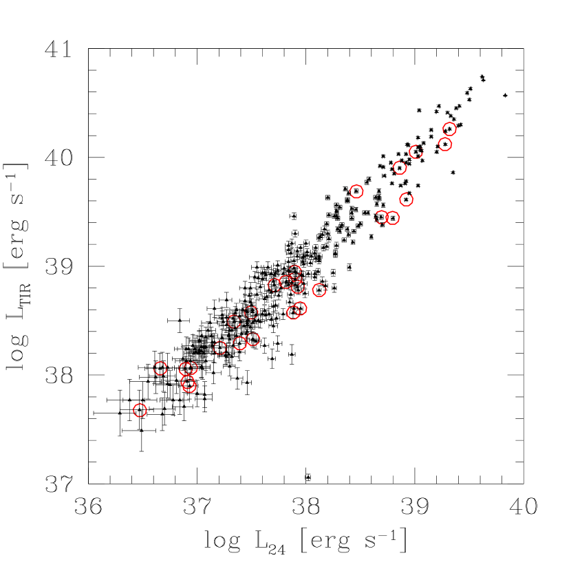
Figure 3: The total infrared luminosity of sources in the main sample as a function of the 24$\mu$m luminosity derived according to Eq.1. Circles mark sources which belong to the isolated sample.

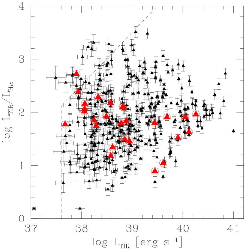
Figure 4: Ratio of the TIR to H$\alpha$ luminosity as a function of the TIR luminosity for IR selected sources. An average value A${}_{V}=1\pm 0.25$ mag has been used to correct the H$\alpha$ luminosity for extinction. The TIR luminosity has been inferred using Eq.1. Circles mark sources which belong to the isolated sample. Dashed lines mark the completeness limits of our survey.

2.3 UV photometry: the round sample and the isolated sample

We now complement the infrared and H$\alpha$ photometry with the far- and near-UV data. UV colors can also be used to infer the age of 24$\mu$m selected sources. GALEX-UV images of M33 are available (Gil de Paz et al. 2007) and we shall use them at the original resolution (1.5 arcsec) to measure the FUV and NUV luminosities of 24 $\mu$m sources with H$\alpha$ counterparts. Because we perform the UV photometry using a circular aperture, we select 106 sources at 24 $\mu$m using the requirement that the PSF ellipticity is less than 0.2. We shall call this the round sample. We set the radius of the UV photometric aperture equal to the source size at 24 $\mu$m and consider an annulus with a width equal to 2 pixels (3 arcsec for GALEX) around sources for background removal. It is not desirable to perform individual UV source extraction because of crowding due to the high density of UV sources. As pointed out already in previous papers (e.g. Calzetti et al. 2005), the UV emission peaks are sometimes displaced with respect to the infrared emission peaks. Stellar complexes can be made of 2 or more populations of different ages, both visible in the UV, with the older ones more extended than the young ones. In this case the old ones should be included in the background. We would like to measure only the UV flux coming from the same area covered by IR emission. To strengthen our results we have selected a clean sample, made of 26 sources that have a clean annulus in both the FUV and NUV images, i.e. no source contamination for background subtraction. We shall call this the isolated sample. Briefly, the sources in the isolated sample are sources from the main sample which satisfy the following criteria: $(i)$ the PSF of the source at 24$\mu$m is nearly circular i.e. the ellipticity is $<\leavevmode\nobreak\ 0.2$ and all of the UV flux is inside $R_{s}$; $(ii)$ the source has one H$\alpha$ counterpart (as defined earlier in this paper); $(iii)$ in the far- and near-UV maps, an annulus of 2 pixels around the emitting source is devoid of any sources.

We will use the round sample, which includes the isolated sample, in the rest of the paper to understand some basic properties of young stellar clusters in M33. To check that we are not oversubtracting the background in the case of sources which do not have a clean annulus, we compute the average UV luminosities for the isolated sample and for the ensemble of sources in the round sample which are not in the isolated sample. The ratio between the two average luminosities is close to unity, being 38.556 and 38.365 the FUV and NUV logarithmically averaged luminosities (in erg s^-1) in the round and non-isolated sample, and 38.563 and 38.377 respectively for the isolated sample. We are therefore confident in the ability of our technique for UV background removal to recover the UV luminosities associated with young clusters.

The UV AB-magnitudes were converted to luminosities using:

$$L_{UV}=\nu F_{\nu}4\pi D^{2}$$ (2)

with $D$ the distance to M33, $\nu=1.9510^{15}$ Hz for the FUV band, $\nu=1.310^{15}$ Hz for the NUV band, and

$${F_{\nu}\over Jy}=10^{23-(AB+48.6)/2.5}.$$ (3)

Considering that the GALEX flux calibration has been revised after the early data release, we apply the recommended 0.12 magnitude offset to the FUV-NUV color defined as $\log\left[L_{\lambda}(FUV)/L_{\lambda}(NUV)\right]$ (Bianchi & Efremova 2006). We consider also the small extinction correction, E(B-V)${}_{MW}\simeq 0.04$, from the Milky Way in the direction of M33 (Schlegel et al. 1998). This implies $A_{UV}\simeq 0.3$ for all sources in M33.

3 UV colors, opacity and bolometric luminosities of star-forming regions

The TIR luminosity of HII regions is radiation from young stars absorbed and re-emitted by dust grains. The leftover cluster radiation, not absorbed by grains, is mostly emitted in the UV. We now infer the extinction of the radiation coming from the gas and the stars in the HII regions using the observed infrared-to-far UV ratio. As in Calzetti (2001), we shall use the factor 1.68 to account for the bolometric correction of the stellar emission relative to the FUV.

Since our IR and UV data refer to clusters still embedded in HII regions, the dust optical depth for the stellar continuum radiation is similar to that for the H$\alpha$ line emission. We are not considering the UV light from previous generations of stars. We infer the FUV extinctions after measuring the TIR and FUV source luminosities, and then we relate this to the extinction at other wavelengths as in Calzetti (2001):

$$A_{FUV}=5.7\times\hbox{log}\left({1\over 1.68}{L_{TIR}\over L_{FUV}}+1\right)$$ (4)

$$A_{NUV}=0.72\times A_{FUV}$$ (5)

$$A_{V}=0.3\times A_{FUV}$$ (6)

$$A_{H\alpha}=0.25\times A_{FUV}.$$ (7)

We show in Figure 5 the ratio $L_{TIR}/L_{FUV}$ versus the GALEX color $L_{\lambda}(FUV)/L_{\lambda}(NUV)$ for sources in the round sample. By comparing this Figure with Fig. 9 and 10 of Calzetti et al. (2005), we see that our selected sources have all $\log\left(L_{TIR}/L_{FUV}\right)$ between $-1$ and 1.2, corresponding to $A_{V}<1.7$. The derived value of $A_{V}$ increases on average towards bright sources. The average UV color is on the order 0.3 mag. All sources in the isolated sample and nearly all sources in the round sample have UV colors $>0.2$ mag., i.e. they are younger than 10 Myrs according to the instantaneous burst model for solar metallicity and for a starburst dust distribution (Calzetti et al. 2000). Exact ages will depend on the metallicity, burst model and dust distribution. An extinction curve like the one observed in the Small Magellanic Cloud, as well as the simultaneous presence of newly formed massive stars and an older UV-emitting population, imply even younger ages for H$\alpha$ emitting sources in our selected star-forming regions.

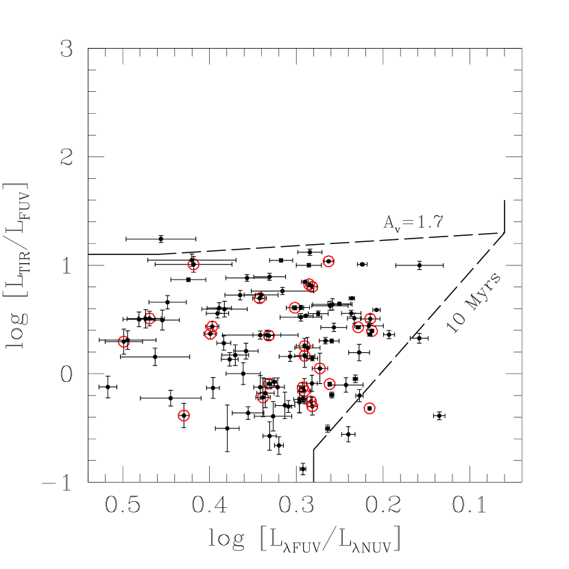
Figure 5: Opacity expressed as infrared-to-FUV luminosity ratio versus the observed UV color for all sources in the round sample. Circles indicates sources in the isolated sample. All sources to the left of the line marked 10 Myrs are younger than 10 Myrs according to the instantaneous burst model. All sources below the mark A${}_{V}=1.7$ have visual extinction A${}_{V}<1.7$ mag.

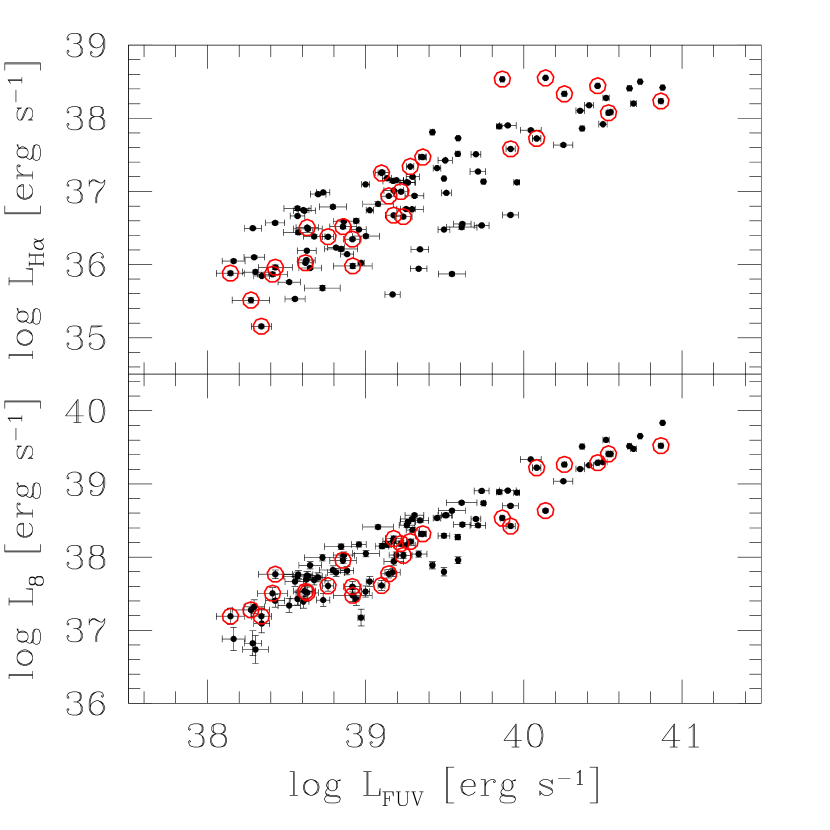
Figure 6: H$\alpha$ and 8$\mu$m luminosities are shown as functions of the FUV luminosities for all sources in the round sample. Circles indicate sources in the isolated sample. Luminosities are in units of erg s^-1; L_Hα and L₈ have been corrected for extinction using the source TIR-to-FUV luminosity ratio.

We estimate the bolometric luminosity of our sources as:

$$L_{bol}=L_{TIR}+[\nu_{FUV}L_{\nu}(FUV)+\nu_{NUV}L_{\nu}(NUV)]$$ (8)

where $\nu_{FUV}$ and $\nu_{NUV}$ are the effective frequencies of the GALEX bands and the UV luminosities are uncorrected for extinction. The bracketed quantity estimates the cluster UV luminosity, between 912 and 3000 Å. In the absence of dust the UV luminosity is a good approximation of the bolometric luminosity for clusters with ages between 1-10 Myr, independent of their mass (as from Starburst99 Leitherer et al. 1999) (see also Bell et al. 2005; Thilker et al. 2007, for similar methods used to estimate L_bol). We shall give another proof in the next Section that indeed our selected clusters fall into this age category. When dust absorb part of the UV radiation and re-irradiate it in the IR, L_TIR is needed in the right hand side of the above equation to correctly estimate L_bol.

We apply extinction corrections to the FUV and H$\alpha$ luminosities of sources in the round sample according to the model described earlier in this Section. The good correlation between extinction corrected UV luminosities and 8$\mu$m luminosities is evident in Figure 6. This is expected since PAHs are excited by the UV radiation of the nearest star-forming region. This nice correlation confirms the goodness of our extinction corrections. Thilker et al. (2007) have found that PAH emission at 8$\mu$m is suppressed within strong star-forming regions. The linear correlation between extinction corrected far-UV luminosities and 8$\mu$m luminosities, which does not break at high luminosities, suggests that this is not happening in M33.

A correlation between FUV and H$\alpha$ luminosities is also present. Given the different dependencies of these two luminosities on cluster mass and age, the presence of some scatter in their relation is not surprising. The next section will better address this issue.

4 The cluster birthline: from bright to dim candles

Because we resolve stars and clusters in M33 at IR and optical wavelengths when the brightest member is earlier than a B2 type star, the expected relation between IR and H$\alpha$ emission is far from linear even under the circumstance that most of the bolometric luminosity of massive stars is absorbed by dust and re-emitted in the IR. This is a result of the different dependencies of the bolometric and H$\alpha$ luminosities on the stellar mass (Panagia 1973; Vacca et al. 1996; Sternberg et al. 2003), considering the lack of the highest mass stars in some clusters. In this Section we would like to investigate in detail the emission by individual clusters at different wavelengths to judge the reliability of using infrared and H$\alpha$ emission as a quantitative tracer of recent star formation for a range of luminosities.

4.1 Modelling cluster birthlines

To compute the H$\alpha$ luminosity of a stellar cluster, one needs to know the mass distribution at the upper end of the IMF. Even though the stellar IMF is well known for intermediate stellar masses, where the original exponent derived by Salpeter (1955) is now widely tested and used, uncertainties remain at the high- and low-mass ends.

The IMF may be interpreted as a probability distribution function that specifies the probability for a randomly chosen star to lie within a certain mass range (e.g. Cerviño & Luridiana 2006; Barker et al. 2008, for stochasticity in the IMF). The absence of stars with very high masses suggests there is a fundamental upper limit to the IMF ($>120-150$ M_⊙ see Massey & Hunter 1998; Elmegreen 2000; Figer 2005; Oey & Clarke 2005; Koen 2006; Hoversten & Glazebrook 2008). The most massive clusters sample the IMF out to this maximum possible stellar mass and no further, even though there are enough stars to do so if the IMF continued with the same slope. Low and intermediate mass clusters do not generally have stars near the maximum possible mass, but their most massive stars tend to have a mass that increases with the cluster mass (Larson 1982). This trend leads to the question of whether the upper limit to the stellar mass in a particular cluster depends on the cluster mass because of some physically limiting process, or whether it follows only from randomly sampling the IMF. In the first case, low mass clusters could not make high mass stars. In the second case they could, as long as there is enough gas, and intermediate-mass clusters should occasionally be found with unusually massive stars – “outliers” in the IMF. An important difference arises for the summed IMF from many clusters: it should be steeper than any cluster IMF in the first case and the same as the average cluster IMF in the second case. The summed IMF is the basis for the present day mass function in whole galaxies and is therefore important to understand for population models and studies of galaxy evolution. A recent debate in the literature suggests the question about maximum stellar mass should be settled observationally (Weidner & Kroupa 2004, 2006; Elmegreen 2006).

In order to model the distribution of stellar masses within a young cluster, we follow two different approaches using the same IMF. In one case we assume that each cluster has a maximum stellar mass that is explicitly related to the cluster mass. We call this the maximum mass case. In the second case, we assume that stars of all masses can form in clusters of all masses, provided there is enough gas, and that the choice of a particular stellar mass is random, following the IMF. We call this the randomly sampled case. Once we specify how a cluster is built we need to establish $L_{bol}^{cl}$ and $L_{H\alpha}^{cl}$, the cluster bolometric and H$\alpha$ luminosity. This is done by summing the contributions of all stars in the cluster using stellar masses, Ly-continuum, and bolometric luminosities tabulated by Vacca et al. (1996) for stellar masses 87.6$<$M$<$19.3 M_⊙ and by Panagia (1973) for 19.3$<$M$<$8 M_⊙. We extrapolate luminosity values logarithmically if stellar masses are outside these mass ranges and interpolate logarithmically for masses that are intermediate to those shown in their tables. We assume ZAMS (Zero Age Main Sequence) and solar metallicity and divide the number of Ly-continuum photon rates by $7.3\times 10^{11}$ ph erg^-1 to obtain H$\alpha$ luminosities.

In what follows we compute the theoretical cluster birthline in the plane log($L_{bol}/L_{H\alpha}$)-log($L_{bol}$) using a stellar IMF with a Salpeter slope $\alpha=-2.35$ between 1 and 120 M_⊙. No stars with mass lower than 1 M_⊙ or higher than 120 M_⊙ will be considered. The IMF in stellar clusters extends down to masses lower than 1 M_⊙ but these stars give a negligible contribution to the cluster luminosity, which is the relevant quantity for this Paper.

In the maximum mass case, given a number N of cluster members with masses above 1 M_⊙, there will be a certain mass limit $M_{N}$ above which the probability of finding one star is unity and this star will be of mass $M_{*}$. If $\xi(M)$ is the number of stars produced per unit mass,

$$\xi(M)dM=CM^{\alpha}dM,$$ (9)

then the number of cluster members with masses above 1 M_⊙, and the cluster mass and luminosity contributed by those stars, can be written as

$$N_{cl}^{>1}=\int_{1}^{120}CM^{\alpha}dM=1+{\int_{1}^{M_{N}}M^{\alpha}dM\over\int_{M_{N}}^{120}M^{\alpha}dM}$$ (10)

$$M_{cl}^{>1}=\int_{1}^{120}CM^{\alpha+1}dM=M_{*}+{\int_{1}^{M_{N}}M^{\alpha+1}dM\over\int_{M_{N}}^{120}M^{\alpha}dM}$$ (11)

$$L_{cl}^{>1}=\int_{1}^{120}CL(M)M^{\alpha}dL=L(M_{*})+{\int_{1}^{M_{N}}L(M)M^{\alpha}dL\over\int_{M_{N}}^{120}M^{\alpha}dM}.$$ (12)

We computed the normalization constant $C$ by assuming that the number of stars between 120 M_⊙ and M_N is unity and we considered the IMF from M_N to 1 M_⊙ as a continuous distribution function with $\alpha=-2.35$ (e.g. Weidner & Kroupa 2006, and references therein). We computed the cluster masses and luminosities in this way for a sequence of clusters with maximum stellar masses corresponding to ZAMS stars of spectral types B2, B1, …. O4, and O3. We set M_N equal to the mass of these stars and consider also that M_∗, the mass of the star born in the mass range M_N–120 M_⊙, is equal to the lower limit of this range, M_N. Statistically M_N is the most likely value for mass in the interval M_N–120 M_⊙, but the assumption that for a given cluster mass no stars are ever made with M$>$M_N is stronger. In Figure 7 we plot with filled circles the cluster birthline made with the maximum mass assumption. That is, each filled circle corresponds to a spectral type in the above sequence, with the corresponding bolometric-to-H$\alpha$ cluster luminosity ratio on the ordinate and the bolometric luminosity on the abscissa for clusters that have a maximum stellar mass with that spectral type.

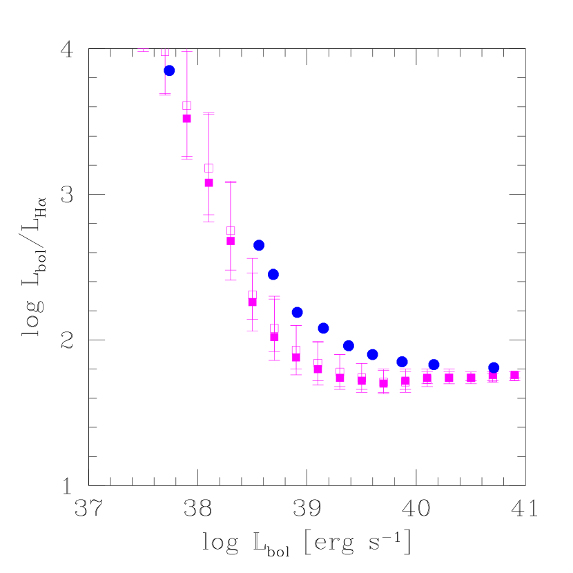
Figure 7: Filled circles mark the expected values of the bolometric-to-H$\alpha$ luminosity ratio for the maximum mass case. Open and filled squares are the mean and median values respectively of the same ratio for the randomly sampled case using a cluster mass function index of $\delta=-2$. Errorbars point out the dispersions around the mean and median values.

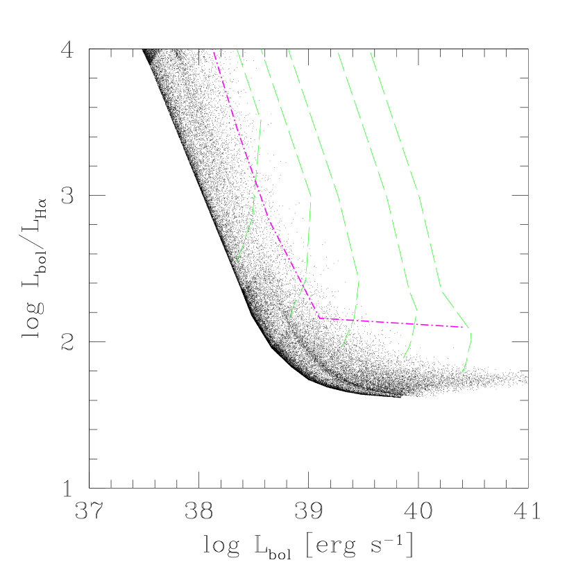
Figure 8: The distribution of the ratio of the bolometric-to-H$\alpha$ luminosity versus the bolometric luminosity for newly born clusters simulated in the randomly sampled case. Vertical dashed lines mark evolutionary sequences, i.e., aging moves clusters upward from the simulated birthline because H$\alpha$ luminosities fade away more rapidly than bolometric luminosities. Clusters reach the top of the plot (L_bol/L${}_{H\alpha}\simeq 4$) in about 10 Myrs. The dash-dotted lines are indicative of when the most massive stars in a cluster leave the main sequence.

In the randomly sampled case, there is no explicit relationship between cluster mass and maximum stellar mass as in equations (10)-(12). Even though M_N is the most likely mass for the cluster’s most-massive member, the actual mass can be as large as 120 M_⊙, although the probability that such a massive star actually forms decreases as the cluster mass decreases. To model this case, we simulate 40000 clusters that are distributed in number according to their mass between 20 and 10000 M_⊙ as

$$N(\hbox{ M}_{cl})\hbox{ dM}_{cl}=\hbox{ D}_{cl}\hbox{ M}^{\delta}_{cl}\hbox{ dM}_{cl}$$ (13)

where $D_{cl}$ is a constant and $\delta$ is the spectral index of the ICMF, usually assumed to be $\delta=-2$ (e.g. de Grijs & Parmentier 2007, and references therein). We then populate each cluster with stars, randomly selected from the stellar IMF described above, until the simulated cluster mass gets above the selected cluster mass. We compute the bolometric and H$\alpha$ luminosity of each cluster using the same ZAMS models as in the maximum mass case. Figure 8 shows the resulting distribution of L_bol/L_Hα versus L_bol with one plotted point for each modelled cluster. The lower boundary of the distribution is where single massive stars lie. Our simulation takes into account incomplete clusters, such as single OB associations born in the field or single stars scattered out of loose clusters. Notice the presence of a second edge of high density points in the distribution. This is from a change in slope of the stellar L_Hα-L_bol relation, which produces a cusp in the diagram. In bins of equal size in $\log$ L_bol units, we plot in Figure 7 the average and the median of the distribution for the randomly sampled case and we plot their 1-$\sigma$ values (enclosing 16.5% and 83.5$\%$ of the points in each bin). Notice that the randomly sampled case predicts median values and average values of log L_bol/L_Hα that are below those of the maximum mass case. This is a result of the occasional presence of bright stars or outliers even in low-mass clusters.

If low mass stars form first, a cluster enters the birthline from the top left and follows it down and to the right as L_bol increases. If, instead, massive stars are born at random times during cluster formation, then the cluster can jump down on the simulated birthline and then move towards slightly higher values of L_bol and L_bol/L_Hα. This happens until all of the gas available to fuel star formation is used or SF is quenched by feedback. Cluster aging from the death of massive stars increases the L_bol/L_Hα ratio and then the cluster moves upward from the birthline. This is because the death of massive stars makes the cluster H$\alpha$ luminosity fade away more rapidly than bolometric luminosity. Using the public code Starburst 99, we evaluate how the clusters evolve off the birthline. The vertical dashed lines in Figure 8 show the aging effect. A cluster reaches the top of the Figure in about 10 Myrs. Two fundamental properties of the predicted cluster birthline are: $(a)$ the linear correlation between L_bol and L_Hα, which holds for very young massive clusters (the horizontal part of the birthline), breaks down below a critical value of the cluster bolometric luminosity, depending on the stellar IMF at the high mass-end; $(b)$ all stellar clusters should lie on or above the birthline shown in Figure 7 for the two cases examined.

4.2 The M33 test case for the birthline

If most of the luminosity of young clusters were absorbed by dust and re-irradiated in the IR, then the L${}_{TIR}\simeq$ L_bol data points in the log(L_TIR/L_Hα) – log(L_TIR) plane should all lie above the birthline sequence. However, by looking at Figure 9, which plots the observed values on the birthline plane, we see a clear discrepancy with the birthline theoretical prediction. Many clusters lie below the birthline, for both the maximum mass case and the randomly sampled case. It has to be pointed out that any heavier extinction correction, as well as corrections due to the loss of ionizing photons leaking out of the HII regions, will move the data points further down, toward lower values of L_bol/L_Hα. Since any data point below the birthline is unexplained we must conclude that our assumption, namely that the TIR luminosity traces the bolometric luminosity, is not correct for most of the clusters observed. This discrepancy with the birthline cannot be the result of an unreliable 24$\mu$m - TIR conversion because the dispersion in the 24$\mu$m to TIR luminosity ratio is only about 0.1 in the log. Also recall that individual extinction corrections have been applied to H$\alpha$ luminosities (see Section 3).

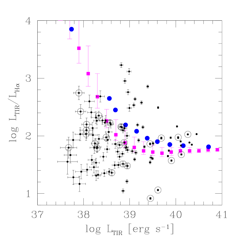
Figure 9: The total infrared-to-H$\alpha$ luminosity ratio for data in the round sample and in the cleanest isolated sample (symbols surrounded by circles). Under the assumption that L_TIR=L_bol, we can compare the cluster data with the predicted cluster birthlines for the randomly sampled case (filled squares) and for the maximum mass case (large filled circles). Individual extinction corrections have been applied to H$\alpha$ luminosities (see Section 3). The selected samples of young clusters is clearly not along or above any birthline, as it should be. Hence the assumption L_TIR=L_bol is incorrect.

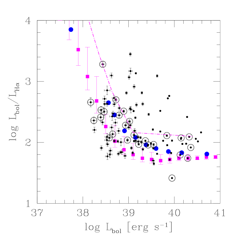
Figure 10: Bolometric to H$\alpha$ luminosity ratio versus bolometric lumosity for data in the round sample and in the cleanest isolated sample (dots surrounded by circles). Bolometric luminosities have been estimated according to Eq. 8 and individual extinction corrections have been applied to H$\alpha$ luminosities (see Section 3). The predicted cluster birthlines for the randomly sampled case (filled squares) and for the maximum mass case (filled circles) are also shown. The dash-dotted line indicates the cluster position when the most massive stars for the randomly sampled case leave the main sequence.

As outlined in the previous Section, we now complement IR with UV photometry to derive the cluster bolometric luminosity. In Figure 10 we plot the $L_{bol}$-to-$L_{H\alpha}$ ratio as a function of $L_{bol}$ for the round sample marking (with circles) members of the isolated sample. Clusters in the round and isolated samples lie above the birthline predicted by the randomly sampled case with a very few exceptions. Members of the isolated sample, for which UV photometry is more accurate, follow closely the birthline and this underlines their young age. Only one cluster in the isolated sample with L${}_{bol}\simeq 10^{40}$ erg s^-1 seems to lie below the birthline, having a lower value of L_bol/L_Hα. The most likely explanation of the H$\alpha$ excess is that this cluster has formed a star more massive than 120 M_⊙, but additional analysis is needed before drawing any definitive conclusion on this. In general the agreement is good also for the round sample: almost all of the clusters lie above the birthline for the randomly sampled case. This implies that the round sample is made up of relatively young clusters too. In Figure 10 we add the main sequence boundary (dash-dotted line). This marks the value of L_bol/L_Hα for a cluster at the end of the main sequence lifetime for single massive stars (e.g. Stahler & Palla 2005). It is impressive how the isolated sample is bounded by the birthline at the bottom and by the main sequence boundary at the top. That means that effectively we have traced the sequence of young compact clusters before supernovae disrupt them and blow away dust grains.

If the birth of stars in clusters is regulated by the statistical character of the IMF and there is no physical or absolute relation between the maximum stellar mass in a cluster and the cluster mass, then the predicted cluster birthline is in good agreement with the data. This agreement is illustrated by the relative number of sources below the birthline, where there should be none. Only 5$\%$ of the clusters are more than 3-$\sigma$ below the birthline in the randomly-sampled case, whereas 25% of the clusters are more than 3-$\sigma$ below the birthline in the maximum-mass case. This result favours the randomly sampled model for the stellar population in clusters.

We infer that some of the clusters with the lowest L_bol/L_Hα ratios for their L_bol values have outlier massive stars, i.e. massive stars without their usual proportion of low mass stars. In these cases, a star has formed with a mass that is larger than the average upper mass limit for a cluster of that mass. It would be interesting to study these cases more to see if there are other unusual characteristics, such as extreme mass segregation, cloud disruption, or cloud temperatures.

Figure 11: Median values for the randomly sampled case obtained using different indices for the cluster distribution function: open squares, filled squares and open triangles correspond to $\delta=-1,-2,-3$ respectively. Filled dots show the data for the round sample. Data for the cleanest isolated sample are surrounded by circles.

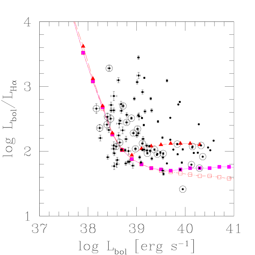
Figure 12: Median values for the randomly sampled case obtained using different index for the stellar IMF: filled triangles, filled squares and open square correspond to $\alpha=-2.80,-2.35,-1.50$. Filled dots show the data for the round sample. Data for the cleanest isolated sample are surrounded by circles.

The simulated L_bol/L_Hα distribution is very marginally dependent on the value of $\delta$ for the cluster mass function. For $-1\leq\delta\leq-3$ the distribution of the median value is within the 1-$\sigma$ error bar values of the more widely used $\delta=-2$ distribution (see Figure 11) (Hunter et al. 2003; Chandar et al. 2006; Dowell et al. 2008). Figure 12 shows the effect of using an IMF index steeper or flatter than the classical Salpeter value. There is a better agreement of some cluster data with a steeper IMF at the high-mass end, but the number of clusters below the birthline increases. So, we favor a Salpeter IMF with some cluster aging to bring them above the birthline. A diagram of L_bol versus UV colors shows that the most luminous sources are also the oldest in our isolated sample. This accounts for the slight rise in plotted points above the birthline for large L_bol in Figure 10. Additional data is needed to better constrain the ages of those clusters.

5 Summary and Discussion

M33 is ideal for deriving the properties of young star-forming clusters and their massive stellar populations. It contains star-forming complexes with a wide range of luminosities, and it is close enough that even clusters with one O- or B-type star can be localized. We have examined in this paper young stellar clusters selected in the 24$\mu$m map of M33 that have H$\alpha$ counterparts. The 8-to-24$\mu$m luminosity ratio has a small dispersion and shows a dependence on the galactocentric radius. The total IR-to-H$\alpha$ luminosity ratio, L_TIR/L_Hα, shows a larger dispersion, especially towards faint sources, and no correlation with galactocentric distance or source IR luminosity. The large scatter in the TIR-to-H$\alpha$ flux arises mostly because of variations in the local dust abundance which adds to some aging effect. Only a certain fraction of the bolometric luminosity of 24$\mu$m-selected sources can be absorbed by grains and re-emitted locally at IR wavelengths. This fraction might be small for low-luminosity sources that are not born along the spiral arms of M33.

We have calculated the bolometric luminosity for 106 “round” stellar clusters, L_bol, using UV and IR photometry. This has allowed us to test the concept of the cluster birthline introduced in this paper. The cluster birthline, defined in the parameter space log(L_bol)–log(L_bol/L_Hα), is the line of birth of young clusters, a theoretical lower boundary for the ratio L_bol/L_Hα for each L_bol. We show that along the cluster birthline the relation between L_bol and L_Hα is linear for high-L_bol clusters but is non-linear for clusters with L${}_{bol}<3\times 10^{39}$ erg s^-1. Deviations from linearity are expected because of two effects: the IMF is not fully sampled in low mass clusters, and the number of photons emitted by a star with energies above the hydrogen ionization threshold has a stronger dependence on stellar mass than does the stellar bolometric luminosity (e.g. Panagia 1973; Vacca et al. 1996). For high L_bol clusters, the IMF is usually sampled out to the highest possible stellar mass and then the ratio of high-to-low mass stars is constant, making the L_Hα to L_bol ratio constant. For low L_bol clusters, the IMF becomes depleted of the highest mass stars; these stars have the lowest ratio of L_bol/L_Hα and their depletion raises the average ratio. The observed flatness of L_bol/L_Hα for luminous sources implies either that there is a maximum possible stellar mass equal to $\sim 120\;M_{\odot}$, as assumed in our models, or that the L_Hα-to-L_bol ratio for individual stars becomes constant at $M>120\;M_{\odot}$.

We modeled the cluster birthline by populating clusters of various masses with stars having masses selected from an IMF. Several cluster mass function slopes and IMF slopes were used for comparison. We modeled the upper end of the IMF in two cases. The maximum mass case assumed that each cluster produced stars with masses only up to a maximum value that equals the average maximum stellar mass for a cluster of that mass. In this case, low mass clusters can produce only low mass stars. The randomly sampled case assumed that each cluster can produce stars over the full range of the IMF, in which case a low mass cluster can occasionally produce a high mass star (provided the cluster mass exceeds the stellar mass, of course). Both cases have the same average maximum stellar mass for clusters of each mass, but only the second case can produce outlier stars – stars with masses significantly above the average maximum for that cluster, which means above the upper end of the smooth and declining part of the IMF that is observed at intermediate stellar mass. Comparing the two cases, the clusters birthline in the maximum mass case has a higher value of L_bol/L_Hα over the range of L_bol where O- and B-type stars are starting to populate the upper end of the IMF. This range extends from L_bol slightly less than $10^{38}$ erg s^-1 to L_bol slightly larger than $10^{40}$ erg s^-1. At smaller L_bol, stars producing H$\alpha$ emission do not form in the maximum mass case and are highly unlikely in the randomly sampled case. At larger L_bol, the IMF is fully sampled in both cases.

From the round sample we selected 26 sources which appear isolated and compact in the UV maps i.e. the annular region around them, used for background subtraction, is not contaminated by UV sources. All but one of the stellar clusters in this sample, called the isolated sample are compatible with cluster birthline predicted in the randomly sampled case for the Salpeter IMF with maximum stellar mass limit of 120 M_⊙. For the isolated sample in fact 25 out of 26 clusters lie on or above this birthline. Considering the whole round sample we find similar fractions: 100 over 106 clusters are compatible with the same birthline. In contrast, 25% of the clusters in the round sample lie below the theoretical birthline in the maximum mass case, and hence are incompatible with this cluster population model. M33 has therefore provided a positive test to the cluster birthline concept introduced in this paper. Stellar clusters are born along the birthline and aging moves the clusters above it. The observations also suggest that stars randomly sample the IMF and that clusters occasionally have outlier massive stars. Clusters in the isolated sample lie below the upper main sequence boundary ($t\leq 3-4$ Myr), which is consistent with their compactness and young age. Below this boundary, the most massive stars that a cluster formed are still present (assuming that all stars form at about the same time), so L_bol/L_Hα remains low, and supernovae have not yet disrupted the cluster or blown away the dust. No cluster in the isolated sample lies above the upper main sequence boundary, but some clusters in the more numerous round sample do. This difference might indicate that some members of the round sample have lost their most massive stars. However, in the opacity–UV-color diagram, the two samples occupy the same area so their ages are about the same. An alternative explanation for the high L_bol/L_Hα ratio is then leakage of ionizing photons from HII regions. Clusters in the round sample are in fact not as compact and isolated as the clusters in the isolated sample, so the non-isolated clusters could be more prone to leakage. Future studies that resolve individual stars should help to answer this age-versus-leakage question. If massive stars are observed directly, and in proportional to the IMF, then leakage must be the cause of the higher L_bol/L_Hα ratio.

Luminosities at 8 and 24$\mu$m correlate with gas metal abundances; the dispersion is large because there are few sources with an accurate metal abundance determination. While we did not find a significative sample of 24$\mu$m sources embedded in GMCs which are not detected in H$\alpha$, we find 34 sources associated with GMCs which have an H$\alpha$ counterpart. The 24$\mu$m luminosities of these sources correlate with associated GMC masses, even though with a large scatter.

From studies in the solar neighborhood we know that a stellar cluster in its youngest stage is likely to be deeply embedded in molecular clouds. Later, mechanical and radiative effects of the most massive stars disrupt the cloud, the extinction decreases and the cluster becomes visible in the ultraviolet. The time interval in which massive stars are detectable through IR, H$\alpha$ and UV emission depends not only on stellar lifetimes but also on the opacity of the parent cloud and on its time evolution. The characteristics of molecular clouds seem linked to the large-scale morphology of the galaxy. Earlier studies of a radio-selected sample of thermal sources in M33 have provided 11 young, optically-visible stellar clusters but no embedded star cluster (Buckalew et al. 2006). A small sample of compact infrared selected sources with no H$\alpha$ counterpart has been observed in the CO J=1-0 and J=2-1 lines (Corbelli et al. 2009, in preparation). The weakness or absence of CO lines suggests that these sources are not embedded proto-stellar clusters in the process of formation but a more evolved population. In M33 the amount of extinction seems generally lower than in the Milky Way. The absence of large molecular complexes and a steeper mass spectrum implies that even in an early SF phase many stellar complexes may not be highly obscured. Later, winds and SN explosions remove efficiently the dusty envelope and the cluster fades away in the IR before less massive stars get off the main sequence.

The concept of a cluster birthline together with the high resolution of future telescopes seems a promising way to analyze star formation in external galaxies.

Appendix A The metallicity and GMC samples

We now investigate if properties of star-forming sites in M33 are related to the host gas metallicity or to the parent molecular cloud mass. We first consider a sample of HII regions observed by Magrini et al. (2007b) for which metallicities have been determined via optical spectroscopy. Extinction can be estimated via the Balmer decrement, even though this is only an upper limit to the overall extinction through a whole HII region. Unfortunately the sample of HII regions with known metallicity for which radio continuum or Paschen lines are available for determining the extinction deeply into the star-forming region is limited to 5 bright sources and therefore the sample is not statistically meaningful. Our metallicity sample is made of 31 HII regions with known O/H abundance, Balmer decrement, and accurate IR photometry at 8 and 24 $\mu$m. H$\alpha$ emission has been corrected for extinction using the Balmer decrement and the relation $A_{V}=1.2\times A_{\rm H\alpha}$. The extinction (which gives values $A_{V}<1.7$ in the whole sample) is comparable to what has been derived with more accurate estimates. There is no trend of extinction with metallicity or with gas column density that is associated with the source site. Low column density gas hosts preferentially low metallicity HII regions.

Figure 13: Metallicity as a function of galactocentric radius for sources with IR counterparts. Filled dots represent sources where the electron temperature diagnostic lines have been detected. The metallicity measured in terms of O/H from a compilation by Magrini et al. (2007a, b) is also plotted as a function of the ratios of the 24$\mu$m to the H$\alpha$ luminosities, and the 24$\mu$m to the 8$\mu$m luminosities. Error bars in log(O/H) are given in Magrini et al. (2007a, b) and are on the order 0.1. Error bars in the luminosity ratios are smaller than the symbol sizes.

Figure 14: The metallicity measured in terms of O/H from a compilation of Magrini et al. (2007a, b) is plotted as a function of the 24$\mu$m, 8$\mu$m, and H$\alpha$ luminosities for sources with IR counterparts. Filled dots represent sources where the electron temperature diagnostic lines have been detected. Error bars in log(O/H) are given in Magrini et al. (2007a, b) and are on the order 0.1. Error bars in the luminosity ratios are smaller than the symbol sizes.

The sample of sources with IR counterparts shows a shallow radial metallicity gradient (Fig. 13). If we restrict our sample to sources where the electron temperature diagnostic lines have been detected, and hence the electron temperature can be measured (filled dots in Figures 13 and 14), then the gradient is compatible with that derived by Magrini et al. (2007b) using the same selection criteria. The $L_{24}/L_{8}$ and $L_{24}/L_{H\alpha}$ ratios do not show any clear metallicity dependence because sources with high metallicity (say O/H above $-3.5$) have high luminosities at optical and IR wavelengths (Fig. 14). The dependence is however very marginal if we consider only sources with electron temperature determinations, whose metallicities are more certain. The scatter around the mean values increases as the metallicity decreases, but this might be an effect of large galactocentric radii, where most of the low metallicity regions are found.

IR luminosities show a dependence on metallicity. Bright sources at 8 and 24$\mu$m are born where metallicity is high while low metallicity gas host a wider range of source luminosities. However uncertainties in the metallicities of bright sources that have no detections of the electron temperature diagnostic lines are large and do not allow us to draw firm conclusions.

Figure 15: The molecular cloud masses associated with the IR selected sources are shown versus the 24$\mu$m luminosities and and the ratios between this luminosity and the H$\alpha$ luminosity.

We also analyze the BIMA giant molecular cloud dataset ($13^{\prime\prime}$ spatial resolution; Engargiola et al. 2003) to see if any sources in the main sample are associated with GMCs and in these cases if the source luminosities are related to the parent GMC masses. Figure 15 shows the GMC masses as functions of the $L_{24}$ and $L_{24}/L_{H\alpha}$ values for sources within 6.5 arcseconds of a GMC. This limiting radius was chosen to match the BIMA spatial resolution of the Engargiola et al. (2003) GMCs survey that was used to identify the clouds. There is a dependence of the IR source luminosity on the GMC mass, despite the large scatter. The slope of the correlation is 0.17$\pm 0.05$ with Pearson linear correlation coefficient of 0.53. The ratio $L_{24}/L_{H\alpha}$ for the GMC sample varies by about 1.5 order of magnitudes for sources associated with small clouds, and by even less for sources associated with the most massive clouds. Sources in the GMC sample are then confined to a smaller range of $L_{24}/L_{H\alpha}$ than that reported in Figure 15 for the full sample. The ratio $L_{24}/L_{H\alpha}$ shows no clear dependence on the GMC mass.

References

- Barker et al. (2008) Barker, S., de Grijs, R., & Cerviño, M. 2008, A&A, 484, 711
- Bell et al. (2005) Bell, E. F., Papovich, C., Wolf, C., et al. 2005, ApJ, 625, 23
- Bertin & Arnouts (1996) Bertin, E. & Arnouts, S. 1996, A&AS, 117, 393
- Bianchi & Efremova (2006) Bianchi, L. & Efremova, B. V. 2006, AJ, 132, 378
- Buckalew et al. (2006) Buckalew, B. A., Kobulnicky, H. A., Darnel, J. M., et al. 2006, ApJS, 162, 329
- Calzetti (2001) Calzetti, D. 2001, PASP, 113, 1449
- Calzetti et al. (2000) Calzetti, D., Armus, L., Bohlin, R. C., et al. 2000, ApJ, 533, 682
- Calzetti et al. (2005) Calzetti, D., Kennicutt, Jr., R. C., Bianchi, L., et al. 2005, ApJ, 633, 871
- Cannon et al. (2006) Cannon, J. M., Walter, F., Armus, L., et al. 2006, ApJ, 652, 1170
- Cerviño & Luridiana (2006) Cerviño, M. & Luridiana, V. 2006, A&A, 451, 475
- Chandar et al. (2006) Chandar, R., Fall, S. M., & Whitmore, B. C. 2006, ApJ, 650, L111
- Corbelli (2003) Corbelli, E. 2003, MNRAS, 342, 199
- Corbelli & Schneider (1997) Corbelli, E. & Schneider, S. E. 1997, ApJ, 479, 244
- de Grijs & Parmentier (2007) de Grijs, R. & Parmentier, G. 2007, Chinese Journal of Astronomy and Astrophysics, 7, 155
- Deul & van der Hulst (1987) Deul, E. R. & van der Hulst, J. M. 1987, A&AS, 67, 509
- Dowell et al. (2008) Dowell, J. D., Buckalew, B. A., & Tan, J. C. 2008, AJ, 135, 823
- Elmegreen (2000) Elmegreen, B. G. 2000, ApJ, 539, 342
- Elmegreen (2006) Elmegreen, B. G. 2006, ApJ, 648, 572
- Engargiola et al. (2003) Engargiola, G., Plambeck, R. L., Rosolowsky, E., & Blitz, L. 2003, ApJS, 149, 343
- Engelbracht et al. (2005) Engelbracht, C. W., Gordon, K. D., Rieke, G. H., et al. 2005, ApJ, 628, L29
- Figer (2005) Figer, D. F. 2005, Nature, 434, 192
- Freedman et al. (1991) Freedman, W. L., Wilson, C. D., & Madore, B. F. 1991, ApJ, 372, 455
- Galliano et al. (2003) Galliano, F., Madden, S. C., Jones, A. P., et al. 2003, A&A, 407, 159
- Gil de Paz et al. (2007) Gil de Paz, A., Boissier, S., Madore, B. F., et al. 2007, ApJS, 173, 185
- Heyer et al. (2004) Heyer, M. H., Corbelli, E., Schneider, S. E., & Young, J. S. 2004, ApJ, 602, 723
- Hippelein et al. (2003) Hippelein, H., Haas, M., Tuffs, R. J., et al. 2003, A&A, 407, 137
- Hogg et al. (2005) Hogg, D. W., Tremonti, C. A., Blanton, M. R., et al. 2005, ApJ, 624, 162
- Hoopes & Walterbos (2000) Hoopes, C. G. & Walterbos, R. A. M. 2000, ApJ, 541, 597
- Houck et al. (2004) Houck, J. R., Charmandaris, V., Brandl, B. R., et al. 2004, ApJS, 154, 211
- Hoversten & Glazebrook (2008) Hoversten, E. A. & Glazebrook, K. 2008, ApJ, 675, 163
- Hunter et al. (2003) Hunter, D. A., Elmegreen, B. G., Dupuy, T. J., & Mortonson, M. 2003, AJ, 126, 1836
- Hunter et al. (2001) Hunter, D. A., Kaufman, M., Hollenbach, D. J., et al. 2001, ApJ, 553, 121
- Israel et al. (1986) Israel, F. P., de Boer, K. S., & Bosma, A. 1986, A&AS, 66, 117
- Israel et al. (1982) Israel, F. P., Gatley, I., Matthews, K., & Neugebauer, G. 1982, A&A, 105, 229
- Israel & Kennicutt (1980) Israel, F. P. & Kennicutt, R. C. 1980, Astrophys. Lett., 21, 1
- Kennicutt (1998) Kennicutt, Jr., R. C. 1998, ApJ, 498, 541
- Kennicutt et al. (2007) Kennicutt, Jr., R. C., Calzetti, D., Walter, F., et al. 2007, ApJ, 671, 333
- Koen (2006) Koen, C. 2006, MNRAS, 365, 590
- Larson (1982) Larson, R. B. 1982, MNRAS, 200, 159
- Leitherer et al. (1999) Leitherer, C., Schaerer, D., Goldader, J. D., et al. 1999, ApJS, 123, 3
- Lu et al. (2003) Lu, N., Helou, G., Werner, M. W., et al. 2003, ApJ, 588, 199
- Magrini et al. (2007a) Magrini, L., Corbelli, E., & Galli, D. 2007a, A&A, 470, 843
- Magrini et al. (2007b) Magrini, L., Vílchez, J. M., Mampaso, A., Corradi, R. L. M., & Leisy, P. 2007b, A&A, 470, 865
- Massey & Hunter (1998) Massey, P. & Hunter, D. A. 1998, ApJ, 493, 180
- Oey & Clarke (2005) Oey, M. S. & Clarke, C. J. 2005, ApJ, 620, L43
- Panagia (1973) Panagia, N. 1973, AJ, 78, 929
- Rosenberg et al. (2006) Rosenberg, J. L., Ashby, M. L. N., Salzer, J. J., & Huang, J.-S. 2006, ApJ, 636, 742
- Rosolowsky & Simon (2008) Rosolowsky, E. & Simon, J. D. 2008, ApJ, 675, 1213
- Salpeter (1955) Salpeter, E. E. 1955, ApJ, 121, 161
- Schlegel et al. (1998) Schlegel, D. J., Finkbeiner, D. P., & Davis, M. 1998, ApJ, 500, 525
- Stahler & Palla (2005) Stahler, S. W. & Palla, F. 2005, The Formation of Stars (The Formation of Stars, by Steven W. Stahler, Francesco Palla, pp. 865. ISBN 3-527-40559-3. Wiley-VCH , January 2005.)
- Sternberg et al. (2003) Sternberg, A., Hoffmann, T. L., & Pauldrach, A. W. A. 2003, ApJ, 599, 1333
- Thilker et al. (2007) Thilker, D. A., Boissier, S., Bianchi, L., et al. 2007, ApJS, 173, 572
- Vacca et al. (1996) Vacca, W. D., Garmany, C. D., & Shull, J. M. 1996, ApJ, 460, 914
- Verley et al. (2008) Verley, S., Corbelli, E., Giovanardi, C., & Hunt, L. K. 2008, ArXiv e-prints
- Verley et al. (2007) Verley, S., Hunt, L. K., Corbelli, E., & Giovanardi, C. 2007, A&A, 476, 1161
- Weidner & Kroupa (2004) Weidner, C. & Kroupa, P. 2004, MNRAS, 348, 187
- Weidner & Kroupa (2006) Weidner, C. & Kroupa, P. 2006, MNRAS, 365, 1333
- Wyder et al. (1997) Wyder, T. K., Hodge, P. W., & Skelton, B. P. 1997, PASP, 109, 927