Isothermal vs. isentropic description of protoneutron stars in the Brueckner-Bethe-Goldstone theory

Abstract

We study the structure of hadronic protoneutron stars within the finite temperature Brueckner-Bethe-Goldstone theoretical approach. Assuming beta-equilibrated nuclear matter with nucleons and leptons in the stellar core, with isothermal or isentropic profile, we show that particle populations and equation of state are very similar. As far as the maximum mass is concerned, we find that its value turns out to be almost independent on T, while a slight decrease is observed in the isentropic case, due to the enhanced proton fraction in the high density range.

I Introduction

A protoneutron star (PNS) is formed after a successful supernova explosion and constitutes for several tens of seconds a transitional state to either a neutron star or a black hole pra . Initially, the PNS is optically thick to neutrinos, that is, they are temporarily trapped within the star. The subsequent evolution of the PNS is dominated by neutrino diffusion, which first results in deleptonization and subsequently in cooling. After a much longer time, photon emission competes with neutrino emission in neutron star cooling.

In this paper, we will focus upon the essential ingredient that governs the macrophysical evolution of neutron stars, i.e., the equation of state (EOS) of dense matter at finite temperature. We have developed a microscopic EOS in the framework of the Brueckner-Bethe-Goldstone (BBG) many-body approach extended to finite temperature. This EOS has been successfully applied to the study of the limiting temperature in nuclei big1 ; big2 . The scope of this work is to present results on the composition and structure of these newly born stars with the EOS previously mentioned.

Two new effects have to be considered for a PNS. First, thermal effects which result in entropy production, with values of a few units per baryon, and temperatures up to 30-40 MeV burr ; pons . Second, the fact that neutrinos are trapped in the star, which means that the neutrino chemical potential is non-zero. This alters the chemical equilibrium and leads to compositional changes. Both effects may result in observable consequences in the neutrino signature from a supernova and may also play an important role in determining whether or not a given supernova ultimately produces a cold neutron star or a black hole.

This paper is organized as follows. In Section 2 we briefly illustrate the BBG many-body theory at finite temperature. Section 3 is devoted to the study of the stellar matter composition at constant temperature or entropy, and the resulting EOS. In Section 4 we discuss our results regarding the structure of (proto)neutron stars, in particular their maximum mass. Finally, conclusions are drawn in Section 5.

II The BBG theory at finite temperature

In the recent years, the Brueckner-Bethe-Goldstone perturbative theory book has been extended in a fully microscopic way to the finite temperature case big1 , according to the formalism developed by Bloch and De Dominicis bloch . In this approach the essential ingredient is the two-body scattering matrix $K$, which, along with the single-particle potential $U$, satisfies the self-consistent equations

$$\langle k_{1}k_{2}|K(W)|k_{3}k_{4}\rangle = \langle k_{1}k_{2}|V|k_{3}k_{4}\rangle$$ (1)

$$\hskip-85.35826pt+\;\mathrm{Re}\!\sum_{k_{3}^{\prime}k_{4}^{\prime}}\langle k_{1}k_{2}|V|k_{3}^{\prime}k_{4}^{\prime}\rangle\!{[1\!-n(k_{3}^{\prime})][1\!-n(k_{4}^{\prime})]\over W-E_{k_{3}^{\prime}}-E_{k_{4}^{\prime}}+i\epsilon}\langle k_{3}^{\prime}k_{4}^{\prime}|K\!(\!W\!)|k_{3}k_{4}\rangle$$

and

$$U(k_{1})=\sum_{k_{2}}n(k_{2})\langle k_{1}k_{2}|K(W)|k_{1}k_{2}\rangle_{A}\>,$$ (2)

where $k_{i}$ generally denote momentum, spin, and isospin. Here $V$ is the two-body interaction, $W=E_{k_{1}}+E_{k_{2}}$ represents the starting energy, $E_{k}=k^{2}\!/2m+U(k)$ the single-particle energy, and $n(k)$ is the finite temperature Fermi distribution. We chose the Argonne $V_{18}$ nucleon-nucleon potential wiringa as two-body interaction $V$, supplemented by three-body forces (TBF) among nucleons, in order to reproduce correctly the nuclear matter saturation point $\rho_{0}\approx 0.17~{}\mathrm{fm}^{-3}$, $E/A\approx-16$ MeV. We have adopted the phenomenological Urbana model schi , which consists of an attractive term due to two-pion exchange with excitation of an intermediate $\Delta$ resonance, and a repulsive phenomenological central term. In the BBG approach, the TBF is reduced to a density-dependent two-body force by averaging over the position of the third particle bbb .

In order to simplify the numerical procedure, we introduce the so-called Frozen Correlations Approximation, i.e., the correlations at $T\neq 0$ are assumed to be essentially the same as at $T=0$. This means that the single-particle potential $U_{i}(k)$ for the component $i$ can be approximated by the one calculated at $T=0$. The accuracy of that approximation has been checked in Ref. big1 .

Within this approximation, for a fixed density $\rho=\sum_{k}n(k)$ and temperature $T$, we solve self-consistently Eqs. (1) and (2) along with the equation for the free energy density, which has the following simplified expression

$$f=\sum_{i}\left[\sum_{k}n_{i}(k)\left({k^{2}\over 2m_{i}}+{1\over 2}U_{i}(k)\right)-Ts_{i}\right]\>,$$ (3)

where

$$s_{i}=-\sum_{k}\Big{(}n_{i}(k)\ln n_{i}(k)+[1-n_{i}(k)]\ln[1-n_{i}(k)]\Big{)}$$ (4)

is the entropy density for component $i$ treated as a free gas with spectrum $E_{i}(k)$. Finally, the pressure can be easily calculated as the derivative of free energy with respect to the density, keeping fixed the temperature, i.e.,

$$P=\rho^{2}\Big{(}\frac{\partial(f/\rho)}{\partial\rho}\Big{)}_{T}\>.$$ (5)

III Composition and EOS of hot stellar matter

For hot and neutrino trapped stellar matter containing only nucleons as relevant degrees of freedom, the composition is determined by the requirements of charge neutrality and beta equilibrium, which read explicitly

$$\sum_{i}q_{i}x_{i}+\sum_{l}q_{l}x_{l}=0\>,$$ (6)

$$\mu_{n}-\mu_{p}=\mu_{e}-\mu_{\nu_{e}}=\mu_{\mu}+\mu_{\bar{\nu}_{\mu}}\>.$$ (7)

In the expression above, $x_{i}=\rho_{i}/\rho_{B}$ represents the baryon fraction for the species $i$, $\rho_{B}$ the baryon density, and $q_{i}$ the electric charge. The same holds true for the leptons, labelled by the subscript $l$. It turns out that the dependence on the proton fraction can be approximated by the so-called parabolic approximation parabol , which reads for the free energy as

$$\frac{F}{A}(\rho,x_{p},T)\approx\frac{F}{A}(\rho,x_{p}=0.5,T)+(1-2x_{p})^{2}{F_{\rm sym}}(\rho,T)$$ (8)

being $F_{\rm sym}$ the symmetry energy

$${F_{\rm sym}}(\rho,T)\approx\frac{F}{A}(\rho,x_{p}=0,T)-\frac{F}{A}(\rho,x_{p}=0.5,T)\>.$$ (9)

In the parabolic approximation, the nucleon chemical potentials can be easily calculated as

$$\mu_{n}(\rho,x_{p},T) = \frac{\partial f}{\partial\rho_{n}}=\left[1+\rho\frac{\partial}{\partial\rho}-x_{p}\frac{\partial}{\partial x_{p}}\right]{f\over\rho}\>,$$ (10)

$$\mu_{p}(\rho,x_{p},T) = \frac{\partial f}{\partial\rho_{p}}=\left[1+\rho\frac{\partial}{\partial\rho}+(1-x_{p})\frac{\partial}{\partial x_{p}}\right]{f\over\rho}\>,$$ (11)

whereas the chemical potentials of the noninteracting leptons are obtained by solving numerically the free Fermi gas model at finite temperature. Further details are given in Ref. nic06 .

Because of trapping, the numbers of leptons per baryon of each flavor $l=e,\mu$,

$$Y_{l}=x_{l}-x_{\bar{l}}+x_{\nu_{l}}-x_{\bar{\nu}_{l}}\>,$$ (12)

are conserved on dynamical time scales. Gravitational collapse calculations of the white-dwarf core of massive stars indicate that at the onset of trapping the electron lepton number is $Y_{e}\approx 0.4$, the precise value depending on the efficiency of electron capture reactions during the initial collapse stage. Moreover, since no muons are present when neutrinos become trapped, the constraint $Y_{\mu}=0$ can be imposed. We fix the $Y_{l}$ at those values in the calculations for neutrino-trapped matter.

III.1 Isentropic description of hot stellar matter

As known from dynamical simulations, thermal effects result in an approximately uniform entropy per baryon of $S/A\approx 1-2$ across the star burr . Therefore, within the same theoretical framework, it may be useful to switch from an isothermal to an isentropic description of hot and trapped stellar matter, and compare the respective outcomes. In our approach, we proceed as follows. Once we determine the composition and the free energy per particle $F/A$ at a given density $\rho$, for several values of the temperature $T$, we calculate the entropy per baryon (in units of the Boltzmann constant) from the thermodynamical relationship

$$\frac{S}{A}=-\Big{(}\frac{\partial F/A}{\partial T}\Big{)}_{\rho}\>.$$ (13)

Hence, for fixed $S$, we find how the temperature changes as a function of the density $\rho$, as shown in Fig. 1. The lower curve displays the calculation for $S/A=1$, whereas the upper curve is the calculation for $S/A=2$. We notice that the temperature is a monotonically increasing function of the density, and that the reachable values are larger for larger values of the entropy. We remark that the range of temperatures coincides with the values chosen for the isothermal description of a protoneutron star nic06 .

Following this procedure, we obtain the stellar composition and the corresponding free energy at a given nucleon density $\rho$. Finally, we can calculate the total energy $E/A$ from the thermodynamical relationship

$$\frac{E}{A}(\rho,x_{p},S)=\frac{F}{A}(\rho,x_{p},S)+T(\rho,x_{p})\frac{S}{A}\>,$$ (14)

and the equation of state is

$$P=\rho^{2}\Big{(}\frac{\partial E/A}{\partial\rho}\Big{)}_{S}\>.$$ (15)

The pressure vs. density relationship is the fundamental input for calculating stable configurations of a protoneutron star. These can be obtained from the well-known hydrostatic equilibrium equations of Tolman, Oppenheimer, and Volkov shapiro for the pressure $P$ and the enclosed mass $m$

$${dP(r)\over dr} = -\frac{Gm(r)\varepsilon(r)}{r^{2}}\frac{\big{[}1+{P(r)\over\varepsilon(r)}\big{]}\big{[}1+{4\pi r^{3}P(r)\over m(r)}\big{]}}{1-{2Gm(r)\over r}}\>,$$ (16)

$$\frac{dm(r)}{dr} = 4\pi r^{2}\varepsilon(r)\>,$$ (17)

once the EOS $P(\varepsilon)$ is specified, being $\varepsilon$ the total energy density ($G$ is the gravitational constant). For a chosen central value of the energy density, the numerical integration of Eqs. (16) and (17) provides the mass-radius relation. For simplicity, we have attached a cold crust to the stellar core, by joining the hadronic equations of state above described with the ones by Negele and Vautherin nv in the medium-density regime ($0.001\;\mathrm{fm}^{-3}<\rho<0.08\;\mathrm{fm}^{-3}$), and the ones by Feynman, Metropolis, and Teller fey and Baym, Pethick, and Sutherland baym for the outer crust ($\rho<0.001\;\mathrm{fm}^{-3}$).

A more realistic treatment of the transition from the hot interior to the cold outer part has a dramatic influence on the mass-central density relation in the region of low central density and low stellar masses, as discussed in Ref. Gondek . However, the maximum mass region is not affected by the structure of this low-density transition region.

IV Results and discussion

Let us now discuss first the populations of beta-equilibrated stellar matter, by solving the chemical equilibrium conditions given by Eqs. (7), supplemented by electrical charge neutrality, and baryon and lepton number conservation.

In Fig. 2 we show the particle fractions as a function of the nucleon density, for different values of the temperature, respectively $T$=20,40 MeV (upper panels), and entropy $S/A$=1,2 (lower panels). We do not observe sizeable differences between the two calculations, except for the neutrino fraction at extremely low densities, and the muon percentage in the high temperature/entropy case.

The equation of state for beta-stable and neutrino trapped matter is displayed in Fig. 3, where the pressure is reported as a function of the nucleon density. We observe that the equation of state stiffens with increasing $T$ or $S$ mostly in the medium-low density range. On the contrary, at large density thermal effects play a minor role, and curves of different $T$ or $S$ show a quite similar behavior, as already found in Ref. nic06 .

Finally, in Fig. 4 we display the gravitational mass as function of the radius (left panels), and the central energy density $\epsilon$ normalized with respect to the saturation value $\epsilon_{0}$ (right panels). The dashed (dot-dashed) line represents the calculations for the low (high) temperature or entropy case. We find that the values of the maximum mass are quite stable and almost independent on $S$ or $T$. In particular, we observe that the value of the maximum mass slightly decreases with increasing $S$. The reason is that in hot and trapped stellar matter, the proton fraction increases with increasing $S$ or $T$ at large values of the nucleon density, and this leads to a softening of the equation of state, with consequent decrease of the maximum mass. This result is in contrast with the findings of Prakash et al. pra , where the critical mass increases with increasing entropy. This can be due to the fact that in Ref. pra the interaction is mostly local, with only a non-local correction, and therefore only the kinetic part contains a dependence on temperature. In our calculations the whole interaction part is temperature-dependent, due to the intrinsic non-locality of the single-particle potentials, and therefore the temperature dependence can be quite different.

In the same figure we also show the results for cold neutrino-free neutron stars (thin solid line). One notes in particular that the maximum masses of the protostars are always slightly smaller than that of the neutron star, which excludes a delayed collapse while cooling down pra ; pons .

V Conclusions

We have modeled nucleonic protoneutron stars using a realistic BBG equation of state and assuming either isothermal or isentropic conditions. Heavy protostars are fairly insensitive to that choice and their maximum masses are slightly smaller than that of the cold neutron star.

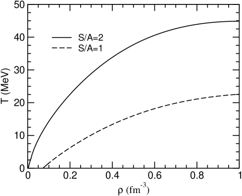
Figure 1: Temperature vs. nucleon density for neutrino-trapped matter with entropy S/A=1 (dashed line) and S/A=2 (solid line).

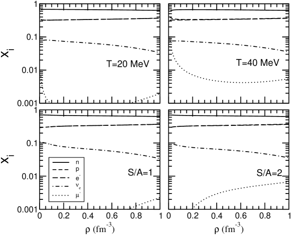
Figure 2: Relative populations for neutrino-trapped matter as a function of the nucleon density. Calculations are shown for the isothermal case (upper panels), and for the isentropic one (lower panels).

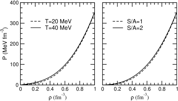
Figure 3: Pressure as a function of the nucleon density for the isothermal case (left panel) and the isentropic one (right panel).

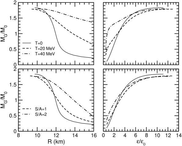
Figure 4: Mass-radius (left panels) and mass-central density (right panels) relations for isothermal (upper panels) and isentropic (lower panels) conditions.

References

- (1) M. Prakash, I. Bombaci, M. Prakash, P.J. Ellis, J.M. Lattimer, and R. Knorren, Phys. Rep. 280, 1 (1997).
- (2) M. Baldo and L.S. Ferreira, Phys. Rev. C59, 682 (1999).
- (3) M. Baldo, L.S. Ferreira, and O. Nicotra, Phys. Rev. C69, 034321 (2004).
- (4) A. Burrows and J.M. Lattimer, Ap. J. 307, 178 (1986).
- (5) J.A. Pons, S. Reddy, M. Prakash, J.M. Lattimer, and J.A. Miralles, Ap. J. 513, 780 (1999).
- (6) M. Baldo, Nuclear Methods and the Nuclear Equation of State (World Scientific, Singapore, 1999).
- (7) C. Bloch and C. De Dominicis, Nucl. Phys. 7, 459 (1958); Nucl. Phys. 10, 181 (1959); Nucl. Phys. 10, 509 (1959).
- (8) R.B. Wiringa, V.G.J. Stoks, and R. Schiavilla, Phys. Rev. C51, 38 (1995).
- (9) J. Carlson, V.R. Pandharipande, and R.B. Wiringa, Nucl. Phys. A401, 59 (1983); R. Schiavilla, V.R. Pandharipande, and R.B. Wiringa, Nucl. Phys. A449, 219 (1986).
- (10) M. Baldo, I. Bombaci, and G.F. Burgio, Astron. Astrophys. 328, 274 (1997).
- (11) I. Bombaci and U. Lombardo, Phys. Rev. C44, 1892 (1991).
- (12) O.E. Nicotra, M. Baldo, G.F. Burgio, and H.-J. Schulze, Astron. Astrophys. 451, 213 (2006).
- (13) S.L. Shapiro and S.A. Teukolsky, Black Holes, White Dwarfs, and Neutron Stars, (John Wiley & Sons, New York, 1983).
- (14) J.W. Negele and D. Vautherin, Nucl. Phys. A207, 298 (1973).
- (15) R. Feynman, F. Metropolis, and E. Teller, Phys. Rev. 75, 1561 (1949).
- (16) G. Baym, C. Pethick, and D. Sutherland, Ap. J. 170, 299 (1971).
- (17) D. Gondek, P. Haensel, and J.L. Zdunik, Astron. Astrophys. 325, 217 (1997).