Lattice Green’s function approach to the solution of the spectrum of an array of quantum dots and its linear conductance

Abstract

In this paper we derive general relations for the band-structure of an array of quantum dots and compute its transport properties when connected to two perfect leads. The exact lattice Green’s functions for the perfect array and with an attached adatom are derived. The expressions for the linear conductance for the perfect array as well as for the array with a defect are presented. The calculations are illustrated for a dot made of three atoms. The results derived here are also the starting point to include the effect of electron-electron and electron-phonon interactions on the transport properties of quantum dot arrays. Different derivations of the exact lattice Green’s functions are discussed.

I Introduction

Quantum dots, quantum wires, and molecular structures are among the most studied low-dimensional condensed matter systems due to their importance to nanoelectronics,dots and recently to biology.biology In the field of molecular electronics, molecules are used to control the current flow when they are assembled in between metal contacts. molecular Among the several physical properties exhibited by low-dimensional electron systems, interesting ones can be found in the transport properties of these systems, such as conductance quantization and conductance oscillations,kwapinski the latter effect depending on the number of atoms in the wire. Some of these effects have been found in the related field of carbon nanotubes, where experiments have shown that the conductance of a single wall carbon nanotube is quantizedliang and shows Fabry-Perot interference patterns, a signature of coherent transport in the carbon wire.

The above systems all fall under the study of low-dimensional physics and are best described starting from the tight-binding approximation. When we address the physical properties of these low-dimensional systems there are two different questions to address. One is concerned with the electronic spectrum,onipko1 and the other with the transport properties.onipko2 The first of these properties is of importance for the optical response of the system and the second for its use in nanoscopic devices.

The need of an efficient method of computing both the spectrum and the conductance of these systems is therefore obvious. Both these problems can be traced back to the calculation of the lattice Green’s function of the system. In the case of the spectrum, the Green’s function should be computed for the isolated system, whereas when considering the transport properties, the Green’s function must be computed taking into account the effect of the coupling between the system and the metallic leads. The lattice Green’s function method was used to describe the appearance of surface modes (Tamm states) in a finite one-dimensional chain and its interaction with a non-linear impurity. molina The generalization to a semi-infinite square lattice was also discussed. molina2 Several different methods of computing transport properties of one-dimensional quantum wires, using lattice Green’s functions, are available in the literature. A tutorial overview on some of the used methods was recently written by Ryndyk et al..ryndyk Using the Keldysh method, the coherent transport through a one-dimensional lattice was studied by Zeng et al..zeng Li et al. studied the transport through a quantum dot ring with four sites.li The inclusion of time dependent potentials on the transport properties of one-dimensional chains was done by Arrachea. arrachea The inclusion of electron-electron interactions in the transport properties of a small system was discussed by OguriOguri and of a quantum wire was done by Karrach et al.,karrach using a functional renormalization group method. The extension to a quasi-one-dimensional Kagomé wire, where the feature of a multiband system is present, was considered by Ishii and Nakayama.ishii The interesting situation where the metallic wire is connected to a Heisenberg chain was studied by Reininghaus et al.. reininghaus The above results are just a very small subset of the existing representative literature on quantum transport, where the concept of lattice Green’s function plays a central role.

Historically, the first approach to electronic transport in a one-dimensional finite system was done in a series of elegant papers published by Caroli et al.. caroli ; combescot ; combescot&schreder In these works the authors addressed the question of how defects affect the charge transport of the quantum wire. Indeed, the question of how localized defects change the otherwise perfect transport properties of the system has been addressed by several authors in the framework of tight-binding systems. Guinea87 ; Sautet88 ; Mizes91

Guinea and Vergés Guinea87 used a Green’s function method to study the local density of states and the localization length of a one-dimensional chain coupled to small pieces of a polymer. They showed that at the band center there is a complete suppression of the transmission coefficient due to a local antiresonance. Sautet and Joachim Sautet88 studied the effect of a single impurity on the transport properties of a one-dimensional chain. The impurity was assumed to change both the on-site energy and the hopping to the next-neighbor atoms. Mizes and Conwell Mizes91 considered the effect of a single impurity in two coupled-chains, showing that a change on the on-site energy has a more pronounced effect in reducing the transmission in the one-dimensional chain than it has in this system. Finally, Peres and Sols studied analytically the effect of a localized defect in the transport properties of polyacene (a multi-band system), putting in evidence a parity effect, that was also used by Akhmerov et al.beenakker to formulate a theory of the valley-valve effect in graphene nanoribbons.peres0 ; peres1 ; castro Also the study of vacancies in transport of quasi-two-dimensional systems is an important area of research.wakabaiashi The study of a linear array of quantum dots, represented by a single site with an $s-$orbital was carried out by Teng et al..teng

The book by Ferry and Goodnick has a very good introductory section to lattice Green’s functions.ferry Also the recursive Green’s function method is there presented. The method we present in this paper has strong similarities to the recursive Green’s function method.ferry The important difference to stress here is that the recursive Green’s function method is implemented as a numerical method, whereas our approach does solve the same type of problems in an analytical way. The link between Green’s functions and transport properties of nanostructures and mesoscopic systems is well covered in the book by Datta.datta

In this work we give a detailed account of a method, based on the solution of the Dyson equation, to compute the lattice Green’s function of an array of quantum dots, where the dot is represented by an arbitrary number of sites with arbitrary values of the site energies and of the hopping parameters. The method is developed within the approximation that there is only one hopping channel between the dots in the array. This constrain is used to keep the level of the formalism at its minimum. The formalism is easily generalized to include the effect of defects (both on-site and adatoms defects) and to describe the transport properties of both the clean and the perturbed system. The method exploits the fact that the Dyson equation for the lattice Green’s function can be solved exactly for bilinear problems as long as the hoppings are not of arbitrary long range. Also the developed formalism can be used to describe surface states and non-linear impurities effectsmolina in a finite array of quantum dots, but we will not pursue these two aspects in this paper. Although developed within a quasi-one-dimensional perspective, we will show in a forthcoming publication how the method can be generalized to two-dimensional ribbons.

II Determination of the lattice Green’s function

In this section we develop a general method for determining the Green’s function of an array of quantum dots. From it both the electronic spectrum and the rule for momentum quantization are obtained. As a warming up we first revisit the solution of the finite chain problem.

The traditional approacheconomou ; barton ; katsura to determine the Green’s function in real space requires the previous solution of the Schrödinger equation, with the corresponding determination of its eigenvalues and eigenvectors. After this is done, the Green’s function is computed using

$$G(\mathbf{r},\mathbf{r}^{\prime},z)=\sum_{n}\frac{\psi_{n}^{\ast}(\mathbf{r})\psi_{n}(\mathbf{r}^{\prime})}{z-\lambda_{n}}$$ (1)

where $\psi_{n}(\mathbf{r})$ and $\lambda_{n}$ are, respectively, the eigenstates and eigenvalues of the eigenproblem $H\psi_{n}(\mathbf{r})=\lambda_{n}\psi_{n}(\mathbf{r})$, where $H$ stands for the Hamiltonian of the problem and the summation over $n$ means a discrete sum (for discrete eigenvalues),or an integration (for continuous eigenvalues), or both, over the quantum numbers of the problem.

The evaluation of the sum in Eq. (1) may be a very hard task, depending on the mathematical complexity of both the wave functions and the eigenvalues. Even for relatively simple cases the evaluation of the summation is far from obvious (see appendices of Ref. lindenberg, ).

An alternative approach, used for lattice systems, starts from the definition of the resolvent operator

$$\hat{G}=\frac{1}{z-H}\,,$$ (2)

and computes the matrix elements of the resolvent by evaluating directly a number of determinants associated with the matrix $(z-H)$. karadov ; teng This method has the obvious drawback of being limited by the possibility of computing analytically the necessary determinants. vein ; dy

We present in what follows a method that overcomes the technical difficulties above mentioned.

II.1 The single chain case

In order to understand how the method works, we revisit the problem of determining the Green’s function of a finite one-dimensional chain of atoms, with a single orbital per atom. This simple example will help us to fix the notation and state the general arguments about the solution of this type of problems. Let us assume that the system has $N$ atoms, with the motion of the electrons described by the tight-binding Hamiltonian

$$H=H_{0}+V\,,$$ (3)

with

$$H_{0}=\epsilon_{0}\sum_{i=1}^{N}|i\rangle\langle i|\,,$$ (4)

and

$$V=-t\sum_{i=1}^{N-1}(|i\rangle\langle i+1|+|i+1\rangle\langle i|)\,.$$ (5)

Clearly, Eq. (4) represents the on-site energy of the electrons in the atoms and Eq. (5) represents the hopping of the electrons between neighboring atoms. This may seem as an important restriction, but it can in fact be relaxed and the approach extended to more general hopping processes. loly Alternatively the Green’s function of a more complex Hamiltonian may be generated using the extension theory for lattice Green’s functions. schwalm

Let us now introduce two different resolvent operators, the free resolvent

$$\hat{G}^{0}=\frac{1}{z-H_{0}}\,,$$ (6)

and the full resolvent $\hat{G}$, given by Eq. (2) with $H$ given by Eq. (3). The strategy is to determine $\hat{G}$ by solving exactly Dyson’s equation,economou considering the hopping term $V$ as perturbation. In terms of the resolvents and of $V$, the Dyson equation takes the form

$$\hat{G}=\hat{G}^{0}+\hat{G}^{0}V\hat{G}\,.$$ (7)

Forming matrix elements with the basis vectors and using $\hat{\mathbf{1}}=\sum_{i=1}^{N}|i\rangle\langle i|$, one obtains

$$\frac{1}{G^{0}}\langle i|\hat{G}|j\rangle=\delta_{ij}-t(\langle i-1|\hat{G}|j\rangle+\langle i+1|\hat{G}|j\rangle)\,,$$ (8)

with $G^{0}=(z-\epsilon_{0})^{-1}$ . Apart from the term $\delta_{i,j}$, this is the equation for the wavefunction of a particle of coordinate $i$ with the tight binding Hamiltonian (3), and eigenvalue $G^{0}(z)$. It is obvious that the difference of two solutions of this equation will be a solution of the equation without the $\delta_{i,j}$ term. So $G_{i,j}\equiv\langle i|\hat{G}|j\rangle$ can be determined by adding a general solution of the homogeneous equation to one particular solution of the full equation. The latter can then be determined by the boundary conditions.

The solutions of the homogeneous equation are superpositions of plane waves, $\langle n|\hat{G}|m\rangle=A_{m}e^{i\theta n},$ where $A_{m}$ is an arbitrary function of $m$, and $\theta$ is defined by

$$\frac{1}{G^{0}}=-2t\cos\theta\,,$$ (9)

the usual dispersion relation for a 1D tight-binding problem with nearest neighbor hopping. To find one particular solution of the full equation, we use the fact that it has to satisfy the homogeneous equation for $i<j$ and $i>j$ and therefore be a linear combination of plane waves of wavevectors $\pm\theta$—the solutions of Eq.(9)—or, equivalently, of $\sin(i\theta)$ and $\cos(i\theta)$:

$$G_{ij}^{<}=A^{j}\cos(i\theta)+B^{j}\sin(i\theta),\textrm{for}\hskip 14.22636pti\leq j\,,$$ (10a)

$$G_{ij}^{>}=C^{j}\cos(i\theta)+D^{j}\sin(i\theta),\textrm{for}\hskip 14.22636pti>j\,.$$ (10b)

In the linear system of equations obtained by fixing $j$ in Eq. (8) ,

$$\left[\begin{array}[]{cccccc}1&tG^{0}&0&\cdots&\cdots&0\\ tG^{0}&1&tG^{0}&0&\cdots&0\\ 0&tG^{0}&1&tG^{0}&\cdots&0\\ \vdots&\ddots&\ddots&\ddots&\ddots&\vdots\\ \vdots&\ddots&\ddots&\ddots&\ddots&\vdots\\ 0&\cdots&\cdots&\cdots&tG^{0}&1\end{array}\right]\left[\begin{array}[]{c}\langle 1|\hat{G}|j\rangle\\ \langle 2|\hat{G}|j\rangle\\ \vdots\\ \langle j|\hat{G}|j\rangle\\ \vdots\\ \langle N|\hat{G}|j\rangle\end{array}\right]=\left[\begin{array}[]{c}0\\ 0\\ \vdots\\ G^{0}\\ \vdots\\ 0\end{array}\right]$$ (11)

all but two equations are automatically satisfied by the fact that $G_{ij}^{<}$ and $G_{ij}^{>}$ solve the homogeneous equation, leaving only two conditions mixing $G_{ij}^{<}$ with $G_{ij}^{>}$:

$$\frac{1}{G^{0}}G_{jj}^{<} = 1-t\left(G_{j+1j}^{>}+G_{j-1j}^{<}\right)\,,$$ (12a)

$$\frac{1}{G^{0}}G_{j+1j}^{>} = -t\left(G_{j+2j}^{>}+G_{jj}^{<}\right).$$ (12b)

These are easily shown to be equivalent (using the fact that the Green’s function is also a solution of the homogeneous equations) to

$$G_{jj}^{>} = G_{jj}^{<}\,,$$ (13a)

$$G_{j+1j}^{>}-G_{j+1j}^{<} = \frac{1}{t}\,.$$ (13b)

The Equation (13a) corresponds to the continuity of the Green’s function, whereas Eq. (13b) corresponds to the discontinuity of the derivative of the Green’s function in the theory of second order differential equations. barton

Inserting Eqs.(10) in Eqs.(13) , one can obtain a rather simple solution (valid in both domains $i\leq j$ and $i>j$) as

$$G_{ij}=\frac{1}{2t\sin\theta}\sin\left(\theta\left|i-j\right|\right)$$ (14)

The general solution is obtained by adding an arbitrary solution of the homogeneous equation,

$$G_{ij}=A^{j}\cos(\theta i)+B^{j}\sin(\theta i)+\frac{1}{2t\sin\theta}\sin\left(\theta\left|i-j\right|\right).$$ (15)

The free coefficients, $A^{j}$ and $B^{j}$, are determined by boundary conditions. For a finite chain we must enforce,

$$\langle 0|\hat{G}|j\rangle=\langle N+1|\hat{G}|j\rangle = 0$$ (16a)

$$\langle i|\hat{G}|0\rangle=\langle i|\hat{G}|N+1\rangle = 0.$$ (16b)

It is straightforward to show that these lead to

$$G_{ij}(z) = \frac{1}{2t}\frac{\cos(N\theta+\theta)}{\sin(N\theta+\theta)\sin\theta}[\cos(i\theta-j\theta)-\cos(i\theta+j\theta)]$$ (17)

$$- \frac{1}{2t}\left[\frac{\sin(i\theta+j\theta)}{\sin\theta}-\frac{\sin|i\theta-j\theta|}{\sin\theta}\right]\,.$$

Noticing that the Chebyshev polynomials obey the finite differences equation

$$f_{n-1}(x)+f_{n+1}(x)=2xf_{n}(x)$$ (18)

and have the representationabramowitz

$$T_{n}(\cos\theta) = \cos(n\theta)\,,$$ (19a)

$$U_{n}(\cos\theta) = \frac{\sin(n\theta+\theta)}{\sin\theta}\,,$$ (19b)

we see that our solution (17) is the same obtained for a finite one-dimensional harmonic lattice, bass as it should be. It is worth noticing that the rule for momentum quantization (that is $\theta$) is obtained from the poles of the Green’s function (17), leading to

$$\sin(N+1)\theta=0\Rightarrow\theta_{\ell}=\frac{\pi{\ell}}{N+1}\,,$$ (20)

with ${\ell}=0,1,2,\ldots,N-1$.

Rewriting $G^{0}=(z-\epsilon_{0})^{-1}$ as $G^{0}=(E-\epsilon_{0}+i0^{+})^{-1}$, where $E$ stands for the energy of the electron, the energy dependence of the Green’s function is obtained;economou this allows the calculation of the local density of states from

$$\rho_{ii}(E)=-\frac{1}{\pi}\Im G_{ii}(E+i0^{+})\,.$$ (21)

It is clear that $\rho_{ii}(E)$ is site dependent for a finite chain. It is an elementary calculation to find an explicit expression for $\rho_{ii}(E)$, by writing both $\cos(2i\theta)$ and $\sin(2i\theta)$ in terms of $\sin\theta$ and $\cos\theta$ and using Eq. (9). We conclude by stressing that the matrix elements of the resolvent were obtained without the need of evaluating the sum over the eigenstates, as in Eq. (1), which constitutes the major advantages of this method over most of the existing ones.

As a final comment in this section, we remark that the final solution for $G_{ij}$ is quite symmetrical in both coordinates, even though the method we followed treats the two coordinates on a rather different footing. In Appendixes A and B we give two other derivations of the Green’s function of a finite chain which treats both coordinates equally from the beginning.

II.2 The general case

We now consider the case where $N$ quantum dots, represented by hexagons in Fig. 1, are coupled together by an hopping parameter $t$. Although having just a single hopping channel between the dots may seem rather restrictive, we used it nevertheless to illustrate the method. Also, if we choose to position the dot in such a way that is has oriented edges such that a particular site of the dot is closer to the next dot than any other point, as in the case of Fig. 1, the used approximation is somewhat justified. The generalization of this possibility to multi-hopping hopping processes does not changes the general idea, but adds some complexity to the final solution. In addition, we assume that the dot is also described by a lattice model. Although this an apparent restriction, it can also be relaxed. We now address the question of determining the Green’s function of the quantum dot array.

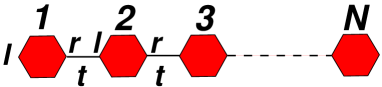
Figure 1: An array of $N$ quantum dots coupled together by an hopping integral $t$. The dot is represented by the hexagon. The points $l$ and $r$ are those that are coupled between dots due to $t$, and the choice of the letters stand for most left and most right points in the dot, respectively.

The Hamiltonian for the problem defined by Fig. 1 is written as

$$H_{T}=H^{D}+V\,,$$ (22)

were

$$H^{D}=\sum_{i=1}^{N}H_{i}^{D}\,,$$ (23)

with $H_{i}^{D}$ the Hamiltonian of the $i$ dot (which is not necessary to specify at this point), and

$$V=-t\sum_{i=1}^{N-1}(|i,r\rangle\langle i+1,l|+|i+1,l\rangle\langle i,r|)\,.$$ (24)

As before we define $\hat{G}^{0}=(z-H^{D})^{-1}$, and note that $|i,\beta\rangle$ are the basis states with $i=1,2,\ldots,N$ and $\beta$ labeling the sites in the quantum dot; we will need two different $\beta$’s only, $\beta=r,l$.

The matrix elements of the Dyson’s equation (8), given the Hamiltonian (22), reads

$$\langle i,\alpha|\hat{G}|j,\beta\rangle=\delta_{i,j}G_{\alpha\beta}^{0} - t(G_{\alpha l}^{0}\langle i-1,r|\hat{G}|j,\beta\rangle$$ (25)

$$+ G_{\alpha r}^{0}\langle i+1,l|\hat{G}|j,\beta\rangle)\,,$$

with $G_{\alpha\beta}^{0}=\langle i,\alpha|\hat{G}^{0}|i,\beta\rangle$. It is easy to see, by direct replacement, that the homogeneous Dyson’s equation (that is when $i\neq j$) is solved by an Ansatz of the form $G_{\alpha\beta}^{nm}=A_{\alpha\beta}^{m}e^{in\theta}$ when $\theta$ is chosen such that

$$1+2tG_{lr}^{0}\cos\theta+t^{2}(G_{lr}^{0})^{2}=t^{2}G_{ll}^{0}G_{rr}^{0}\,,$$ (26)

an expression that gives the band structure once the quantized values of $\theta$ have been determined. We see from Eq. (25) that $\langle i,\alpha|\hat{G}|j,\beta\rangle$ is only coupled to $\langle i-1,r|\hat{G}|j,\beta\rangle$ and $\langle i+1,l|\hat{G}|j,\beta\rangle$. Therefore we will solve the Dyson’s equation (25) for the particular case of $\alpha,\beta=l,r$. To start with we make the Ansatz (a linear combination of terms of the form $A_{\alpha\beta}^{m}e^{in\theta}$)

$$G_{\alpha\beta}^{<,ij}=A_{\alpha\beta}^{<}\cos(i\theta)+B_{\alpha\beta}^{<}\sin(i\theta),\textrm{for}\hskip 14.22636pti<j\,,$$ (27a)

$$G_{\alpha\beta}^{>,ij}=A_{\alpha\beta}^{>}\cos(i\theta)+B_{\alpha\beta}^{>}\sin(i\theta),\textrm{for}\hskip 14.22636pti>j\,,$$ (27b)

where $G_{\alpha\beta}^{\lessgtr,ij}=\langle i,\alpha|\hat{G}|j,\beta\rangle$, and the multiplicative coefficients of the trigonometric functions depending on $j$. The finiteness of the chain is imposed by the conditions

$$\langle 0,r|\hat{G}|j,\beta\rangle=\langle N+1,l|\hat{G}|j,\beta\rangle=0\,,$$ (28)

and time reversal symmetry implies that

$$\langle i,\alpha|\hat{G}|j,\beta\rangle=\langle j,\beta|\hat{G}|i,\alpha\rangle\,.$$ (29)

The solution of the non-homogeneous Dyson’s equations (that is, when $i=j$) leads to a linear system of equations of the form

$$M\mathbf{v}=\mathbf{b}\,,$$ (30)

with the transpose vectors given by $\mathbf{v}^{T}=[A_{ll}^{>},A_{lr}^{>},B_{rr}^{<}]$ $\mathbf{b}^{T}=[G_{ll}^{0},G_{rr}^{0},0]$ . The matrix $M$ is easily constructed from the non-homogeneous Dyson’s equations and is given in the Appendix C. The solution of the linear system is best accomplished by Cramer’s rule, leading to

$$A_{ll}^{>} = -\frac{G_{ll}^{0}}{P_{L}}\sin(N\theta+\theta)\tilde{P}_{j-1}\,,$$ (31a)

$$A_{lr}^{>} = \frac{tG_{ll}^{0}G_{rr}^{0}}{P_{L}}\sin(N\theta+\theta)\sin(j\theta)\,,$$ (31b)

$$B_{rr}^{<} = -\frac{G_{rr}^{0}}{P_{L}}\tilde{P}_{N-j}\,,$$ (31c)

with $P_{L}=tG_{lr}^{0}\sin\theta\tilde{P}_{L}$ and $\tilde{P}_{x}=tG_{lr}^{0}\sin(x\theta-\theta)+\sin(x\theta)$.

Combining the homogeneous and non-homogeneous equations we can derive the following results

$$G^{<,m-1m}_{rl}-G^{>,m-1m}_{rl}=t^{-1}\,,$$

$$G^{>,m+1m}_{lr}-G^{<,m+1m}_{lr}=t^{-1}\,,$$ (32a)

which combined with time reversal symmetry and one of the non-homogeneous equations leads to the linear system

$$V\mathbf{u}=\mathbf{q}\,,$$ (33)

with $\mathbf{u}^{T}=[A^{>}_{rl},B^{>}_{rl},B^{<}_{lr}]$, and $V$ and $\mathbf{q}$ given in Appendix C. The solution of the linear system gives

$$A^{>}_{rl} = (tP_{L})^{-1}\tilde{P}_{L}\tilde{P}_{m-1}\,,$$ (34a)

$$B^{>}_{rl} = -(tP_{L})^{-1}[\cos(L\theta)+tG^{0}_{lr}\cos(L\theta-\theta)]\tilde{P}_{m-1}\,,$$ (34b)

$$B^{<}_{lr} = (tP_{L})^{-1}[\cos\theta+tG^{0}_{lr}\cos(2\theta)]\tilde{P}_{L-m}\,.$$ (34c)

As we saw before the poles of the Green’s function gives the rule of momentum quantization. In this case the poles correspond to the zeros of $P_{L}$, which leads to an equation for the quantization of $\theta$ that reads

$$tG_{lr}^{0}\sin(N\theta-\theta)+\sin(N\theta)=0\,.$$ (35)

Contrary to the case of the single finite chain, Eq. (35) depends on the energy, and therefore it has to be solved together with Eq. (26). The knowledge of $A_{ll}^{>}$, $A_{lr}^{>}$, $A^{>}_{rl}$, $B^{>}_{rl}$, $B^{<}_{lr}$, and $B_{rr}^{<}$ is all that is necessary to determine all the Green’s functions for this problem. The full form of the Green’s functions is given in Appendix D.

II.3 Explicit results for a particular example

Let us now consider a specific example and work out the energy spectrum and the momentum quantization. For the Hamiltonian of the quantum dot we consider the case where the dot is made of three sites very close together, with a single local orbitalteng associated to each site. The sites are coupled together by a hopping matrix element $t_{\triangle}$. The simpler case of representing the dot by a single site was considered by Teng et al.. teng The Hamiltonian of the dot we are considering reads

$$H_{i}^{D}= -t_{\triangle}\sum_{\alpha=1}^{3}(|i,\alpha\rangle\langle i,\alpha+1|+|i,\alpha+1\rangle\langle i,\alpha|)$$ (36)

$$+\epsilon_{0}\sum_{\alpha=1}^{3}|i,\alpha\rangle\langle i,\alpha|\,,$$

with the boundary condition $\langle i,4|=\langle i,1|$ . What is now necessary is to compute the Green’s function for this system. It just happens that the Green’s function for this system is given by the Green’s function of a finite chain (three sites) with periodic boundary conditions. This can be obtained from the procedure of Sec. II.1 by replacing the boundary conditions (16a) by

$$\langle 1|\hat{G}|j\rangle=\langle N+1|\hat{G}|j\rangle\,,$$ (37)

which leads to

$$G_{ij}= -\frac{1}{2t_{\triangle}}\frac{\sin(N\theta)}{\cos(N\theta)\sin\theta-\sin\theta}T_{i-j}(\cos\theta)$$ (38)

$$+\frac{1}{2t_{\triangle}}U_{|i-j|-1}(\cos\theta)\,.$$

For the Hamiltonian (36) we have $N=3$ and the Green’s functions computed from (38) are given by

$$G_{rr}^{0}=G_{ll}^{0}=G_{11}^{0} = \frac{1}{2t_{\triangle}}\frac{1+2\lambda}{-1+\lambda+2\lambda^{2}}\,,$$ (39a)

$$G_{lr}^{0}=G_{rl}^{0}=G_{12}^{0} = \frac{1}{2t_{\triangle}}\frac{1}{1-\lambda-2\lambda^{2}}\,,$$ (39b)

with $\lambda=(E-\epsilon_{0})/(2t_{\triangle})$. We should note that $G_{11}^{0}$ can be written as

$$G_{11}^{0}=\frac{1}{2t_{\triangle}}\left(\frac{2}{3}\frac{1}{\lambda-1/2}+\frac{1}{3}\frac{1}{\lambda+1}\right)\,,$$ (40)

which means that the eigenvalue $\lambda=-1/2$ is bidegenerate, and that is the fundamental reason why the denominator of the Green’s function is not a cubic polynomial.

We shall now consider the physical relevant case where $t_{\triangle}\gg t$. Within this approximation the solutions of Eq. (26) are given by ($\lambda\neq 1$)

$$\lambda_{1} \simeq -1-\frac{t}{3t_{\triangle}}\cos\theta\,,$$ (41a)

$$\lambda_{2} \simeq \frac{1}{2}+\frac{t\cos\theta}{6t_{\triangle}}-\frac{t}{6t_{\triangle}}\sqrt{3+\cos^{2}\theta}\,,$$ (41b)

$$\lambda_{3} \simeq \frac{1}{2}+\frac{t\cos\theta}{6t_{\triangle}}+\frac{t}{6t_{\triangle}}\sqrt{3+\cos^{2}\theta}\,,$$ (41c)

The values of $\theta$ are obtained from the solution of Eq. (35), which requires the knowledge of $G_{12}^{0}$, which in the approximation of Eq. (41) are given by

$$G_{12}^{0}(\lambda_{1}) \simeq -\frac{t^{-1}}{2\cos\theta}\,,$$ (42a)

$$G_{12}^{0}(\lambda_{2}) \simeq \frac{t^{-1}}{-\cos\theta+\sqrt{3+\cos^{2}\theta}}\,$$ (42b)

$$G_{12}^{0}(\lambda_{3}) \simeq -\frac{t^{-1}}{\cos\theta+\sqrt{3+\cos^{2}\theta}}\,$$ (42c)

The Eq. (35) is trivially solved for the case $\lambda=\lambda_{1}$, giving

$$\theta_{\ell}=\frac{\pi\ell}{N+1}\,,$$ (43)

with $\ell=0,\pm 1,\pm 2,\ldots,N$. The other values of $\theta$ for $\lambda_{2}$ (top sign in Eq. (44)) and $\lambda_{3}$ (bottom sign in Eq. (44)) are obtained as solutions of

$$\cos(N\theta)\sin\theta=\pm\sin(N\theta)\sqrt{3+\cos^{2}\theta}\,,$$ (44)

which for large $N$ reduces to

$$\theta_{\ell}\simeq\frac{\pi\ell}{N}\,,$$ (45)

with $\ell=0,\pm 1,\pm 2,\ldots,N$. This result can be appreciate graphically, by plotting both sides of Eq. (44) on the same graph. Naturally, when $N\rightarrow\infty$, $\theta$ becomes a continuous variable in the interval $\theta\in[-\pi,\pi[$. In Figure 2 we plot the eigenvalues $\lambda_{i}$, given by Eq. (41), using $t/t_{\triangle}=0.1$. The three sites composing the dot originate three energy mini-bands (since $t_{\triangle}\gg t$) in the dot array.

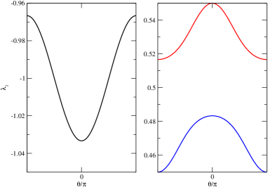
Figure 2: Eigenvalues $\lambda_{i}$, when $i=1$ (left) and $i=2,3$ (right) as function of $\theta/\pi$, for large values of $N$. We have used the ratio $t/t_{\triangle}$=0.1.

It should be now clear that this method allowed us to determine the energy spectrum, the quantization rule for $\theta$, in the case of a finite $N$, and the Green’s functions for the array of quantum dots, with essentially the same effort it would take us to solve the Schrödinger equation for this problem.

III The transport properties

We next want to work out the transport properties of the finite system described in Sec. II.3. We first derive the general results and latter use them to study the system introduced in Sec. II.3. We will consider that our system is connected to two semi-infinite perfect leads. The leads to which we will connect the system will be described in similar terms to those used in the Newns model newns ; davison and the connection between the Green’s function and the transmission across the system is described using a formalism similar to that introduced by Mujica et al.,mujicaI ; mujica ; mujicabook which, it turns out, it is similar to the approach developed by Fisher and Lee. fisher The general relation between the transfer matrix approach and the Green’s function method is described in Ref. [alvarez, ], in the context of continuous models.

III.1 The general formalism

Next we present the general formalism including some particular important results, associated with the concept of surface Green’s function. We represent the Hamiltonian of the perfect leads by one-dimensional semi-infinite tight-binding models reading

$$H_{L} = -\beta_{L}\sum_{i=-\infty}^{0}(|i-1,L\rangle\langle i,L|+|i,L\rangle\langle i-1,L|)\,,$$ (46a)

$$H_{R} = -\beta_{R}\sum_{i=N+1}^{\infty}(|i+1,R\rangle\langle i,R|+|i,R\rangle\langle i+1,R|)\,,$$ (46b)

where $\beta_{L,R}$ are the hopping parameters of the left ($L$) and right ($R$) leads. Although we are representing the leads by a one-dimensional model, this is of no consequences in the characterization of the transport properties of the dots, being only essential that $\beta_{L,R}$ are such that metal bands in the leads have very large band-width. Since the effective band width of our dot structure is proportional to $t$, the only condition is that $\beta_{L,R}\gg t$. The coupling between the leads and the dots is made by the Hamiltonians

$$V_{L} = t_{L}(|0,L\rangle\langle 1,l|+|1,l\rangle\langle 0,L|)\,,$$ (47a)

$$V_{R} = t_{R}(|N+1,R\rangle\langle N,r|+|N,r\rangle\langle N+1,R|)\,,$$ (47b)

where $t_{L,R}$ are the hopping parameters coupling the left ($L$) and right ($R$) leads to the array of quantum dots. We are neglecting the possibility of direct coupling between the left and right leads, a simplification of no physical consequences, corresponding to the fact that the array of dots has many of these. The approach we are formulating with Eqs. (46) and (47) differs somewhat from that of Refs. [newns, ; mujicaI, ], but in general terms the two approaches are perfectly equivalent.

The important aspect of the tunneling approach proposed in Ref. [mujicaI, ] is the need to compute the off-diagonal Green’s function $G_{lr}^{1N}(z)$ for accessing the tunneling properties of the system, including in the calculation the coupling to the semi-infinite leads. This can be done in many different ways [mujicaI, ; teng, ; ando91, ; khomyakov05, ; peressols, ; nikolic, ], leading in the end to results similar to those obtained using non-equilibrium Green’s function methods. jauho ; rammer

The full Hamiltonian of the problem is the sum of Eqs. (22), (46), and (47). Among the several ways available to compute $G_{lr}^{1N}(z)$, one possibility is to use again the Dyson’s equation approach. This requires that we know the exact Green’s function of the leads, before the coupling to the system is established, this is we need to compute the Green’s function of the problem defined by Eq. (46). The calculation of the Green’s function of the leads can be done using the same method we used in Sec. II.1, but now with the boundary conditions

$$\langle 1|\hat{G}_{L}|m\rangle=\langle N|\hat{G}_{R}|m\rangle=0\,.$$ (48)

In this case, however, it is much easier to obtain the Green’s function from the usual definition (1). The wave function of the electrons is given by (let us consider the left lead only)

$$|\theta\rangle=\sqrt{\frac{2}{N_{L}+1}}\sum_{n=-N_{L}}^{0}\sin[(n-1)\theta]|n\rangle\,,$$ (49)

where $N_{L}$ is a normalization length that is taken to infinity in the end of the calculation. Using the definition (1) and the wave function (49) the matrix elements of the resolvent is given by the integral in the complex plane (where $C$ defines a contour over the unit circle $w=e^{i\theta}$)

$$G_{nm,L}(z)=\frac{1}{2\pi i}\oint_{C}\frac{w^{|n-m|}-w^{|m+n-2|}}{\beta_{L}w^{2}+zw+\beta_{L}}dw\,.$$ (50)

The integral in (50) can be evaluated using the same method it has been used to solve for the Green’s function of a chain with periodic boundary conditions economou , leading to

$$G_{nm,L}^{ret}(E)=\frac{1}{2i\beta_{L}}(1-x^{2})^{-1/2}\left(w_{2}^{|n-m|}-w_{2}^{|m+n-2|}\right)\,,$$ (51)

with $G_{nm,L}^{ret}(E)$ standing for the retarded Green’s function, $w_{2}=-x+i\sqrt{1-x^{2}}$ and $x=E/(2\beta_{L})$, such that $|x|<1$. The result (51) is a generalization of the particular results given in Ref. [bishop, ] [the same is true for Eq. (52)]. Repeating the same arguments for the right lead we obtain

$$G_{nm,R}^{ret}(E)=\frac{1}{2i\beta_{R}}(1-x^{2})^{-1/2}\left(w_{2}^{|n-m|}-w_{2}^{|m+n-2N|}\right)\,,$$ (52)

and $x=E/(2\beta_{R})$. Central to our study are the surface Green’s functions $G_{00,L}^{ret}(E)$ and $G_{N+1N+1,R}^{ret}(E)$ which we obtain from Eqs. (51) and (52).

In order to determine $G_{lr}^{1N}(z)$ we introduce $H^{0}=H_{L}+H_{T}+H_{R}$ and the full Hamiltonian $H=H^{0}+V_{L}+V_{R}$, the free resolvent is $\hat{G}^{0}=(z-H^{0})^{-1}$. As before, $G_{lr}^{1N}(z)$ is determined solving the Dyson’s equation, which due to the short range nature of $V_{L}$ and $V_{R}$ has an analytical solution, reading

$$G_{lr}^{1N}(z)=\langle 1l|\hat{G}^{0}|Nr\rangle D^{-1}\,,$$ (53)

with

$$D = (1-t_{L}^{2}\langle 1l|\hat{G}^{0}|1l\rangle G_{00,L})$$ (54)

$$\times (1-t_{R}^{2}\langle Nr|\hat{G}^{0}|Nr\rangle G_{N+1N+1,R})$$

$$- t_{L}^{2}t_{R}^{2}\langle 1l|\hat{G}^{0}|Nr\rangle\langle Nr|\hat{G}^{0}|1l\rangle G_{00,L}G_{N+1N+1,R}\,.$$

A formally equivalent result to Eq. (53) was first derived by Caroli et al., caroli in the context of tunneling across a one-dimensional wire, which was the first application of the Keldyshrammer formalism to tunneling problems.

Let us now describe briefly the calculation of the linear conductance, for which Eq. (53) is needed. The central quantity in this approach is the $T-$matrix. Starting from the Dyson’s equation (7) and introducing an iterative solution, we arrive at an equivalent form for $\hat{G}$, given by

$$\hat{G}=\hat{G}^{0}+\hat{G}^{0}\hat{T}\hat{G}^{0}\,,$$ (55)

where $\hat{T}$ is the $T-$matrix given by

$$\hat{T}=V+V\hat{G}^{0}\hat{T}=V+V\hat{G}V\,,$$ (56)

which describes the scattering of an electron from an initial state $|i\rangle=|0L\rangle$ in the left lead, to a final state $|f\rangle=|N+1R\rangle$ in the right lead. Assuming that the chemical potential difference between the to leads (electron reservoirs) is $\mu_{R}=\mu_{L}+e{\cal V}$, with $e$ the modulus of the electron charge and ${\cal V}$ the electromotive potential between the two reservoirs, the transmission rate is given by

$$\frac{1}{\tau} = \frac{2\pi}{\hbar}\sum_{\alpha,\beta}f(E_{\alpha}^{L}-\mu_{L})[1-f(E_{\beta}^{R}-\mu_{R})]\times$$ (57)

$$|T_{0L,N+1R}|^{2}\delta(E_{\alpha}^{L}-E_{\beta}^{R})\,,$$

where

$$T_{0L,N+1R}=\langle 0L|\hat{T}|N+1R\rangle=\langle 0L|V\hat{G}V|N+1R\rangle\,,$$ (58)

leading to a linear current

$$j=-\frac{e}{\tau} = {\cal V}\frac{2\pi e^{2}}{\hbar}\sum_{\alpha,\beta}(-)\left.\frac{\partial f(x)}{\partial x}\right|_{x=E_{\beta}-\mu_{L}}\times$$ (59)

$$|T_{0L,N+1R}|^{2}\delta(E_{\alpha}^{L}-E_{\beta}^{R})\,.$$

As usual, the conductance is given by $g=j/{\cal V}$. At low temperature, $g$ reads

$$g(\mu_{L}) = \frac{2\pi e^{2}}{\hbar}|T_{0L,N+1R}|^{2}\rho_{L}(\mu_{L})\rho_{R}(\mu_{L})\,$$ (60)

$$= \frac{2\pi e^{2}}{\hbar}t_{R}^{2}t_{L}^{2}|G_{lr}^{1N}(\mu_{L})|^{2}\rho_{L}(\mu_{L})\rho_{R}(\mu_{L})\,.$$ (61)

Naturally, the density of states $\rho_{L}(\mu_{L})$ and $\rho_{R}(\mu_{L})$ should be interpreted as the local density of states at sites 0 and $N+1$, respectively. Equation (61) is formally equal to that derived by Caroli et al., caroli using the Keldysh formalism, and should be multiplied by a factor of two due to the spin of the electrons.

We should stress here that our approach to the tunneling problem is similar to that developed by Mujica et al., mujicaI ; mujica ; mujicabook but not exactly identical. These authors used the Newns couplingnewns of the system to the leads, and their approach to the solution of the Green’s function is based on the properties of tridiagonal determinants after using Löwdin’s partitioning technique,lowdin whereas we explicitly solve the Dyson’s equation.

III.2 Application to a three-sites quantum dot

As an application of the formalism that can be worked out analytically in full detail, we study the transport across a three-sites quantum dot, as that shown in Fig. 3. Although this is a very simple model, it is relevant enough for the our illustrative purposes.

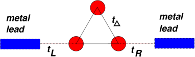
Figure 3: A three-sites quantum dot characterized by $t_{\triangle}$. This is coupled to two metal leads by the couplings $t_{R}$ and $t_{L}$.

The Green’s functions of the quantum dot depicted in Fig. 3 has been computed in Eq. (39), for the case where the coupling to the leads was neglected. Next, we need to compute Eq. (53) for this problem. To this end we need the surface Green’s functions $G_{00,L}$ and $G_{22,R}$, which lead to

$$G_{00,L}^{ret}(E)=G_{22,R}^{ret}(E)=\frac{x}{\beta_{i}}-\frac{i}{\beta_{i}}\sqrt{1-x^{2}}\,,$$ (62)

with $x=E/(2\beta_{i})$, with $i=L,R$. Interesting enough, the local density of states computed from (62), does not diverge at the band edge, as it happens with the density of states of an infinite one-dimensional tight-binding model. economou The calculation of the matrix element of the $T-$matrix leads to

$$|G_{lr}^{1N}(\mu_{L})|^{2}=16t_{\triangle}^{2}\beta^{8}(t_{\triangle}+E-\epsilon_{0})^{2}{\cal D}^{-1}\,,$$ (63)

with ${\cal D}$ given by

$${\cal D}=4(4\beta^{2}-E^{2})\left[(t_{R}^{2}+t_{L}^{2})\beta^{2}(t_{\triangle}^{2}-(E-\epsilon_{0})^{2})\right.$$

$$\left.+t_{R}^{2}t_{L}^{2}E(E-\epsilon_{0})\right]^{2}+\left[2E\beta^{2}(t_{L}^{2}+t_{R}^{2})(-t_{\triangle}^{2}+(E-\epsilon_{0})^{2})\right.$$

$$-2t_{L}^{2}t_{R}^{2}(E^{2}-2\beta^{2})(E-\epsilon_{0})$$

$$\left.+4\beta^{4}(t_{\triangle}+E-\epsilon_{0})^{2}(2t_{\triangle}-E+\epsilon_{0})\right]^{2}\,.$$ (64)

The algebraic form of ${\cal D}$ suggests that for an array of quantum dots, giving a simple analytical form as Eq. (53) may not be possible in general, and the last steps of a given particular calculation may have to be done numerically.

III.3 Defects

In this section we describe the effect of defects on the electronic spectrum of the array of dots as well as on its transport properties. Let us again consider the generic situation described in Fig. 1, and consider as a simple and specific example that at the site $(x,l)$ ($1\leq x\leq N$) there is an adatom. We want to study what is the effect of this adatom on the spectrum of the system and latter on its transport properties. A particular study of the effect of an adatom on the conductance of a quantum wire was done by Kwapiński. kwapinski The presence of the adatom adds an extra term to the Hamiltonian (22) of the form

$$H_{AD}=H_{AD}^{0}+V_{AD}\,,$$ (65)

with

$$H_{AD}^{0} = \epsilon_{\odot}|AD\rangle\langle AD|\,,$$ (66a)

$$V_{AD} = t_{\odot}(|AD\rangle\langle xl|+|xl\rangle\langle AD|)$$ (66b)

where $|AD\rangle$ is the electronic state in the adatom, $t_{\odot}$ is the electronic hopping between the adatom and the $(x,l)$ site of the array, and $\epsilon_{\odot}$ is the local electronic energy in the adatom.

It is again straightforward to apply the Dyson equation formalism to compute the exact Green’s function in the presence of the impurity, leading to

$$\langle n\alpha|\hat{G}|m\beta\rangle=\langle n\alpha|\hat{G}^{0}|m\beta\rangle+\langle n\alpha|\hat{G}^{0}|xl\rangle T\langle xl|\hat{G}^{0}|m\beta\rangle\,,$$ (67)

with the $T$ matrix given by

$$T=t_{\odot}^{2}[z-\epsilon_{\odot}-t_{\odot}^{2}\langle xl|\hat{G}^{0}|xl\rangle]^{-1}\,,$$ (68)

and the matrix elements $\langle n\alpha|\hat{G}^{0}|m\beta\rangle$ are computed from the resolvent $\hat{G}^{0}=(z-H_{T})^{-1}$, with $H_{T}$ defined by Eq. (22). From Equation (67) we can compute Eq. (53) and from this the conductance given by Eq. (61).

In addition, we can compute the Green function of the impurity, determining how the energy level is modified due to the coupling to the bath of electrons propagating along the array. This is given by ($G_{AD}\equiv\langle AD|\hat{G}|AD\rangle$)

$$G_{AD}=[z-\epsilon_{\odot}-t_{\odot}^{2}\langle xl|\hat{G}^{0}|xl\rangle]^{-1}\,.$$ (69)

From Equation (69), the local density of states at the impurity can be computed as $\rho_{AD}=-1/\pi\Im G_{AD}^{ret}$. The accepted $\theta$ values are now the solution of $1/G_{AD}=0$.

III.4 Defects: an application

Again we make a simple application of the formalism of Sec. III.3 considering the system depicted in Fig. 4.

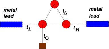
Figure 4: A triangular dot with the atoms coupled together by $t_{\triangle}$, which in turn is coupled to two metal leads by the coupling constants $t_{R}$ and $t_{L}$. An add atom (represented by the square) is connected to one of the atoms of the dot via the hopping $t_{\odot}$.

The $G^{0}$ Green’s functions entering in Eq. (53) are given in this example by

$$G_{ll}^{0} = (\lambda-1/2)(1+2\lambda)(2t_{\triangle}\lambda+\Delta\epsilon){\cal D}^{-1}\,,$$ (70a)

$$G_{rr}^{0} = [(\lambda-1/2)(1+2\lambda)(2t_{\triangle}\lambda+\Delta\epsilon)$$ (70b)

$$- \lambda t_{\odot}^{2}/t_{\triangle}]{\cal D}^{-1}\,,$$

$$G_{lr}^{0} = -(2t_{\triangle}\lambda+\Delta\epsilon){\cal D}^{-1}\,,$$ (70c)

with ${\cal D}$ given by

$${\cal D}=(\lambda-1/2)[2t_{\triangle}(-1+\lambda+2\lambda^{2})(2t_{\triangle}\lambda+\Delta\epsilon)-t_{\odot}^{2}(1+2\lambda)]\,,$$ (71)

with $\Delta\epsilon=\epsilon_{0}-\epsilon_{\odot}$. It is interesting to note that the eigenvalue $\lambda=1/2$ of the non-perturbed triangular dot is not modified by the adatom. The calculation of the conductance is now just a matter of using Eq. (70) in Eq. (53).

IV Discussion

We have presented in full detail a method to compute the lattice Green’s functions of an array of quantum dots for the cases when the array is isolated as well as when it is coupled to two metallic leads. The effect of the leads is to produce a self-energy which has both a real ($\Re\Sigma$) and an imaginary ($\Im\Sigma$) parts. In the case of a single quantum dot, $\Re\Sigma$ will renormalize the energy levels in the dot whereas $\Im\Sigma$ makes the energy levels non-stationary. Both terms contribute to the charge transport through the dot.

The formalism is general and flexible enough to allow for the study of how localized defects affect both the energy spectrum and the transport properties. We can consider both the case when the defect acts as local potential, i.e., diagonal disorder, and when the defect changes locally the values of the hopping integrals, i.e., off-diagonal disorder. Also more than one defect can be attached to the quantum dot array, at different positions in the lattice. In the case of a random distribution of impurities an approximate treatment such as the CPAeconomou can be used to compute the full lattice Green’s function self-consistently.peres0

The generalization of the present approach to two dimensions should present no difficulties, allowing for the possibility to proceed analytically in the calculation of the energy spectrum and transport properties of finite size two-dimensional ribbons. This possibility will be explored in a forthcoming publication. The more restrictive aspect of the method could be related to the calculation of the allowed values of $\theta$, since these are to be computed at the same time the values of the energy eigenvalues are determined. For an array of $N$ dots, each dot having $N_{s}$ sites, the determination of the spectrum following a brute force approach would require the diagonalization of a matrix of dimension $(N_{s}\times N)^{2}$. In our approach this is reduced to the determination of the zeros of a polynomial of degree $N_{s}$. If we consider the case of periodic boundary conditions, the $\theta$ values are given by $\theta_{\ell}=2\pi\ell/N$, with $\ell=0,\pm 1,\pm 2,\ldots N/2$ (assuming $N$ even), and the equation giving the energy spectrum is the same which we would have obtained if we had done a Fourier transform in the initial Hamiltonian.

It important to stress that our approach can easily include the case where the quantum dot is represented by a continuous model. In this case the Green’s function of the dot has the form $G(\mathbf{r},\mathbf{r}^{\prime},E)$, where $\mathbf{r}$ and $\mathbf{r}^{\prime}$ are two-dimensional vectors characterizing the position in the dot. In order to apply the developed formalism we only need to choose the values of $\mathbf{r}$ to which the dots connect among themselves.

Finally we note that our description of the transport is easily generalized to include finite values of the potential bias between the leads. In this case, an appropriate treatment of the problem requires to solve for the Green’s function together with an iterative solution of the Poisson’s equation. For quasi-one-dimensional systems this does not require powerful computational facilities. This will be addressed in a forthcoming publication.

Appendix A An alternative solution of the finite chain problem I

We develop here an approach to the solution of the finite chain problem that builds the symmetries between the two coordinates of the Green function form the start. This method can also be used to tackle the more general problem of the quantum dot array. In terms of the resolvents and of $V$, Dyson’s equation can take two alternative forms,

$$\hat{G} = \hat{G}^{0}+\hat{G}^{0}V\hat{G}\,,$$ (72a)

$$\hat{G} = \hat{G}^{0}+\hat{G}V\hat{G}^{0}\,.$$ (72b)

Forming matrix elements with the basis state vectors and using $\hat{\mathbf{1}}=\sum_{n=1}^{N}|n\rangle\langle n|$, one obtains

$$\langle n|\hat{G}|m\rangle = G^{0}\delta_{nm}$$ (73a)

$$- tG^{0}(\langle n-1|\hat{G}|m\rangle+\langle n+1|\hat{G}|m\rangle)\,,$$

$$\langle n|\hat{G}|m\rangle = G^{0}\delta_{nm}$$ (73b)

$$- tG^{0}(\langle n|\hat{G}|m-1\rangle+\langle n|\hat{G}|m+1\rangle)\,,$$

with $G^{0}=(z-\epsilon_{0})^{-1}$. By taking the sum and the difference of these equations, one derives equivalent conditions which are more symmetrical in the two coordinates of the Green function,

$$\frac{1}{G^{0}}\langle n|\hat{G}|m\rangle = \delta_{nm}-\frac{t}{2}\left(\langle n-1|\hat{G}|m\rangle+\langle n+1|\hat{G}|m\rangle\right.$$ (74a)

$$+ \left.\langle n|\hat{G}|m-1\rangle+\langle n|\hat{G}|m+1\rangle\right)\,,$$

$$0 = \langle n-1|\hat{G}|m\rangle+\langle n+1|\hat{G}|m\rangle$$ (74b)

$$- \langle n|\hat{G}|m+1\rangle-\langle n|\hat{G}|m+1\rangle.$$

Apart from the Kronecker delta term $\delta_{nm}$, Eq. (74a) defines the wavefunction of two particles with a tight-binding Hamiltonian and an eigenvalue $1/G^{0}$. It is obvious that the difference of two solutions of this set of equations will be a solution of the corresponding homogeneous system (without the $\delta_{nm}$ term). Our strategy for finding $\langle n|\hat{G}|m\rangle\equiv G_{nm}$ is the following: (i) we construct the general solution of the homogeneous system assuming plane waves in the two “particle” coordinates; (ii) we find one solution of the full non-homogeneous system, by allowing different plane wave solution for $n\leq m$ and $n>m$, very much in the spirit of the Bethe solution for two particles with local interactions, moving in one dimension; (iii) the general solution is just the particular solution of (ii) added to a general linear combinations of the solutions of (i). To determine the latter we require additional boundary conditions, which, for a finite chain are:

$$G_{0m} = 0\,,$$ (75a)

$$G_{N+1m} = 0\,,$$ (75b)

$$G_{n0} = 0\,,$$ (75c)

$$G_{nN+1} = 0\,.$$ (75d)

We begin by writing a general solution of the homogeneous system in the form

$$\psi_{nm}=Ae^{i\theta_{1}n+i\theta_{2}m}.$$ (76)

Inserting this trial solution in Eq. (74b) we get the condition $\cos\theta_{1}-\cos\theta_{2}=0$; we must have $\theta_{1}=\pm\theta_{2}\equiv\theta$. With this condition, $\psi_{nm}$ is a solution of the homogeneous version of Eq. (74a) provided

$$\frac{1}{G^{0}}=-2t\cos\theta\,.$$ (77)

So the solution of the homogeneous equations is a linear superposition of waves

$$\psi_{nm}(\theta)=Ae^{i\theta(n-m)}+Be^{i\theta(n+m)},$$ (78)

where $\theta$ solves Eq. (77).

We now address the determination of one solution of the full non-homogeneous Eqs. (74), which we write in the form $\phi_{nm}=\psi_{nm}^{<}$, for $n\leq m$, and $\phi_{nm}=\psi_{nm}^{>}$, for $n>m$, where $\psi_{nm}^{<}$ and $\psi_{nm}^{>}$ are two different solutions of the homogeneous system. There are only two conditions that mix $\psi^{<}$ and $\psi^{>}$, namely

$$\frac{1}{G^{0}}\psi_{nn}^{<} = 1-\frac{t}{2}\left(\psi_{n+1n}^{>}+\psi_{n-1n}^{<}+\psi_{nn+1}^{<}+\psi_{nn-1}^{>}\right)\,,$$

$$\frac{1}{G^{0}}\psi_{n+1n}^{>} = -\frac{t}{2}\left(\psi_{n+2n}^{>}+\psi_{nn}^{<}+\psi_{n+1n+1}^{<}+\psi_{n+1n-1}^{>}\right).$$

Because $\psi^{<}$ and $\psi^{>}$ are solutions of the homogeneous system, we can easily transform these conditions into

$$1 = \frac{t}{2}\left(\psi_{n+1n}^{>}-\psi_{n+1n}^{<}+\psi_{nn-1}^{>}-\psi_{nn-1}^{<}\right)\,,$$ (79a)

$$0 = \psi_{nn}^{<}-\psi_{nn}^{>}+\psi_{n+1n+1}^{<}-\psi_{n+1n+1}^{>}\,.$$ (79b)

These conditions cannot be fulfilled by solutions which are function of $n+m$, so we must have:

$$\psi_{nm}^{<} = A^{<}e^{i\theta(n-m)}+B^{<}e^{-i\theta(n-m)}\,,$$

$$\psi_{nm}^{>} = A^{>}e^{i\theta(n-m)}+B^{>}e^{-i\theta(n-m)}\,.$$

Inserting these trial functions in Eqs. (79) and solving the corresponding linear equations for the constants, one gets,

$$A^{<}=-B^{<}=-A^{>}=B^{>}=-\frac{1}{4it\sin\theta},$$

leading to a solution

$$\phi_{nm}=\frac{1}{2t\sin\theta}\sin\left(\theta\left|n-m\right|\right),$$

exactly as found in section II.1, eq,(14) We have now carried out points (i) and (ii) outlined above, and obtained the general solution of Eqs. (74), as

$$G_{nm}=\psi_{nm}+\frac{\sin\left(\theta\left|n-m\right|\right)}{2t\sin\theta}\,,$$

where $\psi_{nm}$ is superposition of waves of the form (78) with $\theta$ satisfying Eq. (77). To enforce the boundary conditions it proves more convenient to write the solution in sines and cosines as

$$G_{nm} = A\cos\left[\theta\left(n-m\right)\right]+B\sin\left[\theta\left(n-m\right)\right]$$

$$+ C\cos\left[\theta\left(n+m\right)\right]+D\sin\left[\theta\left(n+m\right)\right]$$

$$+ \frac{\sin\left(\theta\left|n-m\right|\right)}{2t\sin\theta}\,.$$

To derive the values of these constants, we insert this solution in the Eqs. (75), use the linear independence of the sine and cosine functions and arrive at the final result:

$$G_{nm}(z) = \frac{1}{2t}\frac{\cos\left[\theta\left(N+1\right)\right]}{\sin\left[\theta\left(N+1\right)\right]\sin\theta}$$ (80)

$$\times \left\{\cos\left[\theta\left(n-m\right)\right]-\cos\left[\theta\left(n+m\right)\right]\right\}$$

$$- \frac{1}{2t}\left\{\frac{\sin\left[\theta\left(n+m\right)\right]}{\sin\theta}-\frac{\sin\left[\theta\left|n-m\right|\right]}{\sin\theta}\right\}\,,$$

which is the same solution as Eq. (17).

Appendix B An alternative solution of the finite chain problem II

In the previous appendix, the Dyson equation was written in two alternative forms, see Eqs. (72) and (73).

In Eq. (73a), the ket is unchanged and it can be thought of as a tight-binding equation for the bra of $\langle n|G|m\rangle$ with an inhomogeneity at site $m$. Since we are dealing with a real Hamiltonian, we can make the following ansatz for $G_{n,m}=\langle n|G|m\rangle$:

$$G_{nm}=\left\{\begin{array}[]{cl}G_{nm}^{<}=a_{1}(m)\cos\theta n+a_{2}(m)\sin\theta n&\;,\;n<m\\ G_{nm}^{>}=b_{1}(m)\cos\theta n+b_{2}(m)\sin\theta n&\;,\;n\geq m\end{array}\right.$$ (83)

where $a_{i}(m)$ and $b_{i}(m)$ ($i=1,2$) are arbitrary functions of $m$.

In Eq. (73b), the bra is unchanged and it can be thought of as a tight-binding equation for the ket of $\langle n|G|m\rangle$ with an inhomogeneity at site $n$. We can thus make the following ansatz:

$$G_{nm}=\left\{\begin{array}[]{cl}G_{nm}^{<}=c_{1}(n)\cos\theta m+c_{2}(n)\sin\theta m&\;,\;m>n\\ G_{nm}^{>}=d_{1}(n)\cos\theta m+d_{2}(n)\sin\theta m&\;,\;m\leq n\end{array}\right.$$ (86)

where $c_{i}(n)$ and $d_{i}(n)$ ($i=1,2$) are arbitrary functions of $n$.

Combining Eqs. (83) and (86), we arrive to the following ansatz for the Green’s function:

$$G_{nm}=\left\{\begin{array}[]{cl}G_{n,m}^{<}=a_{1}\cos\theta n\cos\theta m+a_{2}\cos\theta n\sin\theta m+a_{3}\sin\theta n\cos\theta m+a_{4}\sin\theta n\sin\theta m&\;,\;n<m\\ G_{nm}^{>}=b_{1}\cos\theta n\cos\theta m+b_{2}\cos\theta n\sin\theta m+b_{3}\sin\theta n\cos\theta m+b_{4}\sin\theta n\sin\theta m&\;,\;n\geq m\end{array}\right.$$ (89)

Notice that now the coefficients are site-independent.

From the boundary conditions $G_{0m}^{<}=G_{n0}^{>}=0$, we obtain $a_{1}=a_{2}=b_{1}=b_{3}=0$. From the boundary conditions $G_{N+1m}^{<}=G_{nN+1}^{>}=0$, we have $a_{3}=-a_{4}\tan\theta(N+1)$ and $b_{2}=-b_{4}\tan\theta(N+1)$. The matching condition at $n=m-1$ yields $G_{mm}^{<}=G_{mm}^{>}$ (continuity of the Green’s function) and thus $a_{4}=b_{4}$. The matching condition at $n=m$ yields $G_{m-1m}^{<}-G_{m-1m}^{>}=t^{-1}$ (discontinuity of the derivative of the Green’s function) and thus $a_{4}=(\sin\theta\tan\theta(N+1)t)^{-1}$. The final result can therefore be written as

$$G_{nm}^{<} =\frac{1}{t}\frac{-\tan\theta(N+1)\sin\theta n\cos\theta m+\sin\theta n\sin\theta m}{\tan\theta(N+1)\sin\theta}$$

$$=-\frac{1}{t}\frac{\sin\theta(N+1-m)\sin\theta n}{\sin\theta(N+1)\sin\theta}\;,$$ (90)

$$G_{nm}^{>} =G_{mn}^{<}\;.$$ (91)

Again $\theta$ is determined by the dispersion relation Eq. (77). This yields an alternative (but equivalent) representation of the Green’s functions of a tight-binding chain with open boundaries.

The extension to the more general case is analogous, but one has to take special care by defining the matching conditions because the unperturbed Green’s function is now a matrix. It then follows that the Green’s function for the non-diagonal matrix elements which are not constrained by the boundary conditions will be discontinuous for energies which are not eigenenergies of the unperturbed system.

Appendix C Matrix $M$ of Eq. (30) and matrix $V$ of Eq. (33)

The matrix $M$ of Eq. (30) is given by

$$M=\left[\begin{array}[]{ccc}L_{0}+tG_{lr}^{0}L_{1}&tG_{ll}^{0}L_{2}&0\\ 0&tG_{rr}^{0}L_{4}&L_{5}+tG_{lr}^{0}L_{3}\\ tG_{rr}^{0}L_{4}&tG_{lr}^{0}(L_{2}-L_{4})&-tG_{ll}^{0}L_{3}\end{array}\right]\,,$$ (92)

with the functions $L_{i}$, with $i=0,\ldots,5$ given by

$$L_{0} = \cos(m\theta)-\cot(N\theta+\theta)\sin(m\theta)\,,$$ (93a)

$$L_{1} = \cos(m\theta+\theta)-\cot(N\theta+\theta)\sin(m\theta+\theta)\,,$$ (93b)

$$L_{2} = [\cot(m\theta)-\cot(N\theta+\theta)]\sin(m\theta-\theta)\,,$$ (93c)

$$L_{3} = \sin(m\theta-\theta)\,,$$ (93d)

$$L_{4} = \cos(m\theta+\theta)-\cot(N\theta+\theta)\sin(m\theta+\theta)\,,$$ (93e)

$$L_{5} = \sin(m\theta)\,.$$ (93f)

The matrix $V$ of Eq. (33) is given by

$$V=\left[\begin{array}[]{ccc}\cos(m\theta)&\sin(m\theta)&0\\ \cos(m\theta-\theta)&\sin(m\theta-\theta)&0\\ \cos(m\theta+\theta)&a(\theta)&b(\theta)\end{array}\right]\,,$$ (94)

with the functions $a(\theta)$ and $b(\theta)$ given by

$$a(\theta) = \cos(m\theta+\theta)\tan(m\theta)\,,$$ (95a)

$$b(\theta) = \sin(m\theta+\theta)-\cos(m\theta+\theta)\tan(m\theta)\,.$$ (95b)

The vector $\mathbf{q}^{T}=[q_{1},q_{2},q_{3}]$ entering in Eq. (33) has its components given by

$$q_{1} = (tP_{L})^{-1}[tG^{0}_{rl}P_{L}-t^{3}G^{0}_{rl}G^{0}_{rr}G^{0}_{ll}\sin(m\theta-\theta)$$ (96a)

$$\times \sin(N\theta+\theta-m\theta)$$

$$+ t^{2}G^{0}_{rr}G^{0}_{ll}\sin(N\theta-m\theta)\tilde{P}_{m-1})]\,,$$

$$q_{2} = (tP_{L})^{-1}[-P_{L}+t^{2}G^{0}_{rr}G^{0}_{ll}\sin(N\theta+\theta-m\theta)$$ (96b)

$$\times \sin(m\theta-\theta)\,,$$

$$q_{3} = (tP_{L})^{-1}[-P_{L}+t^{2}G^{0}_{rr}G^{0}_{ll}\sin(N\theta-m\theta)$$ (96c)

$$\times \sin(m\theta)\,.$$

Appendix D Full analytical expressions for the Green’s functions

After using the boundary conditions and three of the four time reversal conditions, the Ansatz for the Green’s functions for $n<m$ is

$$G^{nm}_{ll} = A^{<}_{ll}[\cos(n\theta)-\cot(m\theta)\sin(n\theta)]$$ (97a)

$$+ A^{>}_{ll}[\cot(m\theta)-\cot(N\theta+\theta)]\sin(n\theta)\,,$$

$$G^{nm}_{rl} = A^{>}_{lr}[\cot(m\theta)-\cot(N\theta+\theta)]\sin(n\theta)\,,$$ (97b)

$$G^{nm}_{lr} = A^{<}_{lr}\cos(n\theta)+B^{<}_{lr}\sin(n\theta)\,,$$ (97c)

$$G^{nm}_{rr} = B^{<}_{rr}\sin(n\theta)\,,$$ (97d)

and for $n>m$ is

$$G^{nm}_{ll} = A^{>}_{ll}[\cos(n\theta)-\cot(N\theta+\theta)\sin(n\theta)]\,,$$

$$G^{nm}_{rl} = A^{>}_{rl}\cos(n\theta)+B^{>}_{rl}\sin(n\theta)\,,$$ (98a)

$$G^{nm}_{lr} = A^{>}_{lr}[\cos(n\theta)-\cot(L\theta+\theta)\sin(n\theta)]\,,$$ (98b)

$$G^{nm}_{rr} = A^{>}_{rr}[\cos(n\theta)-\cot(m\theta)\sin(n\theta)]$$ (98c)

$$+ B^{<}_{rr}\sin(n\theta)\,.$$

Following the method described in the bulk of the paper, the full analytical expressions for the Green’s functions are given by

$$G_{rr}^{ij}=\left\{\begin{array}[]{c}-\frac{G_{rr}^{0}}{P_{L}}\sin(i\theta)\tilde{P}_{L-j},\hskip 14.22636pti<j\,,\\ -\frac{G_{rr}^{0}}{P_{L}}\sin(j\theta)\tilde{P}_{L-i},\hskip 14.22636pti>j\,,\end{array}\right.$$ (101)

$$G_{ll}^{ij}=\left\{\begin{array}[]{c}-\frac{G_{ll}^{0}}{P_{L}}\sin[(N+1-j)\theta]\tilde{P}_{i-1},\hskip 14.22636pti<j\,,\\ -\frac{G_{ll}^{0}}{P_{L}}\sin[(N+1-i)\theta]\tilde{P}_{j-1},\hskip 14.22636pti>j\,,\end{array}\right.$$ (104)

$$G_{rl}^{ij}=\left\{\begin{array}[]{c}\frac{tG_{rr}^{0}G_{ll}^{0}}{P_{L}}\sin(i\theta)\sin[(N+1-j)\theta],\hskip 14.22636pti<j\,,\\ \frac{1}{tP_{L}}\tilde{P}_{L-i}\tilde{P}_{j-1}\hskip 14.22636pti\geq j\,,\end{array}\right.$$ (107)

and

$$G_{lr}^{ij}=\left\{\begin{array}[]{c}\frac{1}{tP_{L}}\tilde{P}_{L-j}\tilde{P}_{i-1}\hskip 14.22636pti\leq j\,,\\ \frac{tG_{rr}^{0}G_{ll}^{0}}{P_{L}}\sin(j\theta)\sin[(N+1-i)\theta],\hskip 14.22636pti>j\,.\end{array}\right.$$ (110)

Note that $G_{lr}^{ij}=G_{rl}^{ji}$ and that the diagonal Green’s functions obey

$$G_{ll}^{>,i+1i}-G_{ll}^{<,i+1i}=\frac{G_{ll}^{0}}{tG_{lr}^{0}}\,,$$ (111)

$$G_{rr}^{<,i-1i}-G_{rr}^{>,i-1i}=\frac{G_{rr}^{0}}{tG_{rl}^{0}}\,,$$ (112)

which is similar to Eqs. (13b) and (32a), which is the generalization to the lattice of the discontinuity of the first derivative of a Green’s function.

Similar results to those given in this Appendix have been also obtained in Ref. [onipkof, ] in the context of organic molecular systems, but no hints about the method used to derive them was given.

References

- (1) Kenichi Nishi, Device Applications of Quantum Dots, chap. 12. In Y. Masumoto, T. Takagahara, editors, Semiconductor Quantum Dots: Physics, Spectroscopy and Applications, (New York: Springer, 2002) p. 457.
- (2) Charles Z. Hotz and Marcel Bruchez, editors, Quantum Dots: Applications in Biology , (Totowa: Humana Press, 2007).
- (3) Michael C. Petty, Molecular Electronics: From Principles to Practice, (Ames: WileyBlackwell, 2007).
- (4) T. Kwapiński, J. Phys.:Condens. Matter 18, 7313 (2006); idem, ibidem 19, 176218 (2007).
- (5) Wenjie Liang, Marc Bockrath, Dolores Bozovic, Jason H. Hafner, M. Tinkham, Hongkun Park, Nature 411, 665 (2001); Jing Kong, Erhan Yenilmez, Thomas W. Tombler, Woong Kim, Hongjie Dai, Robert B. Laughlin, Lei Liu, C. S. Jayanthi, and S. Y. Wu Phys. Rev. Lett. 87, 106801 (2001).
- (6) Alexander Onipko, Yuriy Klymenko, and Lyuba Malysheva, J. Chem. Phys. 107, 5032 (1997).
- (7) Alexander Onipko, Yuriy Klymenko, and Lyuba Malysheva, Phys. Rev. B 62, 10480 (2000).
- (8) Mario I. Molina, Phys. Rev. B 67, 054202 (2003); idem, ibidem 73, 014204 (2006).
- (9) idem, ibidem 74, 045412 (2006).
- (10) D.A. Ryndyk, R. Gutierrez, B. Song, and G. Cuniberti, arXiv:0805.0628v1.
- (11) Zhao Yang Zeng, Yi-You Nie, F. Claro, and W. Yan, Phys. Lett. A 331, 84 (2004).
- (12) Hua Li, Tianquan Lu, and Punan Sun, Phys. Stat. Sol. (b) 242, 1679 (2005).
- (13) Liliana Arrachea, Phys. Rev. B 72, 125349 (2005).
- (14) Akira Oguri, Phys. Rev. B 63, 115305 (2001).
- (15) C. Karrasch, T. Enss, and V. Meden, Phys. Rev. B 73, 235337 (2006).
- (16) Hiroyuki Ishii and Takashi Nakayama, Phys. Rev. B 73, 235311 (2006).
- (17) Frank Reininghaus, Thomas Korb, and Herbert Schoeller, Phys. Rev. Lett. 97, 026803 (2006).
- (18) C. Caroli, R. Combescot, P. Nozieres, and D. Saint-James, J. Phys. C:Solid St. Phys., 4, 916 (1971); idem, ibidem, 4, 2598 (1971); idem, ibidem, 5, 21 (1972).
- (19) R. Combescot, J. Phys. C:Solid St. Phys., 4, 2611 (1971).
- (20) R. Combescot and G. Schreder, J. Phys. C:Solid St. Phys., 6, 1363 (1973); idem, ibidem, 7, 1318 (1974).
- (21) F. Guinea and J. A. Vergés, Phys. Rev. B 35, 979 (1987).
- (22) P. Sautet and C. Joachim, Phys. Rev. B 38, 12238 (1988).
- (23) H. Mizes and E. Conwell, Phys. Rev. B 44, 3963 (1991).
- (24) N. M. R. Peres and F. Sols, J. Phys.: Condens. Matter 20, 255207 (2008).
- (25) A. R. Akhmerov, J. H. Bardarson, A. Rycerz, and C. W. J. Beenakker, Phys. Rev. B 77, 205416, 2008.
- (26) N. M. R. Peres, F. Guinea, and A. H. Castro Neto, Phys. Rev. B 73, 125411 (2006).
- (27) N. M. R. Peres, A. H. Castro Neto, and F. Guinea, Phys. Rev. B 73, 195411 (2006).
- (28) A. H. Castro Neto, F. Guinea, N. M. R. Peres, Physics World, November, 33 (2006).
- (29) Katsunori Wakabayashi, J. Phys. Soc. Jpn. 71, 2500 (2002).
- (30) B. H. Teng, H. K. Sy, Z. C. Wang, Y. Q. Sun, and H. C. Yang, Phys. Rev. B 75, 012105 (2007).
- (31) David K. Ferry and Stephen M. Goodnick, Transport in Nanostructures, (Cambridge: Cambridge University Press, 2001).
- (32) Supriyo Datta, Electronic Transport in Mesoscopic Systems, (Cambridge: Cambridge University Press, 2005).
- (33) Eleftherios N. Economou, Green’s Functions in Quantum Physics, 3ed (Berlin: Springer-Verlag, 2006).
- (34) G. Barton, Elements of Green’s Functions and Propagation: Potentials, Diffusion and Waves, (Oxford: Oxford University Press, 1989).
- (35) Shigetoshi Katsura, Tohru Morita, Sakari Inawashiro, Tsuyoshi Horiguchi, and Yoshihiko Abe, J. Math. Phys. 12, 892 (1971).
- (36) Katja Lakatos-Lindenberg, Richard P. Hemenger, and Robert M. Pearlstein, J. Chem. Phys. 56, 4852 (1972).
- (37) Peter Karadov and Obis Castaño, J. Mol. Struct. 90, 115 (1982); idem, J. Chem. Soc. Faraday Trans. 2, 78, 73 (1982).
- (38) Robert Vein and Paul Dale, Determinants and Their Applications in Mathematical Physics , (New York: Springer-Verlag, 1998).
- (39) K. S. Dy, Shi-Yu Wu, and T. Spratlin, Phys. Rev. B 20, 4237 (1979).
- (40) A. A. Bahurmuz and P. D. Loly, J. Math. Phys. 22, 564 (1981).
- (41) William A. Schwalm and Mizuho K. Schwalm, Phys. Rev. B 37, 9524 (1988).
- (42) Milton Abramowitz and I. A. Stegun, Handbook of Mathematical Functions, (New York: Dover, 1965).
- (43) Ronald Bass, J. Math. Phys. 26, 3068 (1985).
- (44) Rolando Pérez-Álvarez and Federico García-Moliner, Transfer Matrix, Green Function and Related Techniques, (Castelló de la Plana: Publicaciones de la Universitat Jaume I, 2004).
- (45) D. M. Newns, Phys. Rev. 178, 1123 (1969).
- (46) Sydney G. Davison and Kenneth W. Sulston, Green Function Theory of Chemisorption, (Dordrecht: Springer, 2006) chap. 4.
- (47) V. Mujica, M. Kemp, and M. A. Ratner, J. Chem. Phys. 101, 6849 (1994); idem, ibidem 101, 6856 (1994).
- (48) Vladimiro Mujica, Mathieu Kemp, Adrian Roitberg, and Mark Ratner, J. Chem. Phys. 104, 7296 (1996).
- (49) Vladimiro Mujica, Mathieu Kemp, Adrian Roitberg, and Mark Ratner, A model for Coulomb interaction in electron transport in one-dimensional mesoscopic devices. In E. Ludena, P. Vashishta, R. Bishop, editors, Condensed Matter Theories: Volume 11, (Hauppauge, New York: Nova Sciences Publishers, 1996) pp. 261-272.
- (50) Daniel S. Fisher and Patrick A. Lee, Phys. Rev. B 23, 6851 (1981).
- (51) T. Ando, Phys. Rev. B 44, 8017 (1991).
- (52) P. A. Khomyakov, G. Brocks, V. Karpan, M. Zwierzycki, and P. J. Kelly, Phys. Rev. B 72, 35450 (2005).
- (53) K. Nikolić and A. MacKinnon, Phys. Rev. B 50, 11008 (1994).
- (54) Antti-Pekka Jauho, Ned S. Wingreen, and Yigal Meir, Phys. Rev. B 50, 5528 (1994).
- (55) J. Rammer and H. Smith, Rev. Mod. Phys. 58, 323 (1986).
- (56) Z. G. Yu, D. L. Smith, A. Saxena, and A. R. Bishop, Phys. Rev. B 59, 16001 (1999).
- (57) Per-Olov Löwdin, J. Math. Phys. 3, 969 (1962).
- (58) Alexander Onipko and Lyuba Malysheva, Coherent Electron Transport in Molecular Contacts: a Case of Tractable Modeling, chap. 23. In Sergey Edward Lyshevski, editor, Nano and Molecular Electronics Handbook, (London: CRC, 2007).