Superstatistics of Labour Productivity in Manufacturing and Nonmanufacturing Sectors

Abstract

Labour productivity distribution (dispersion) is studied both theoretically and empirically. Superstatistics is presented as a natural theoretical framework for productivity. The demand index $\kappa$ is proposed within this framework as a new business index. Japanese productivity data covering small-to-medium to large firms from 1996 to 2006 is analyzed and the power-law for both firms and workers is established. The demand index $\kappa$ is evaluated in the manufacturing sector. A new discovery is reported for the nonmanufacturing (service) sector, which calls for expansion of the superstatistics framework to negative temperature range.

¹ Department of Physics, Kyoto University, Kyoto 606-8501, Japan
² NiCT/ATR CIS, Applied Network Science Lab., Kyoto 619-0288, Japan
³ Hitachi Research Institute, 4-14-1 Soto-kanda, Chiyoda-ku, Tokyo, 101-8010, Japan
⁴ Department of Physics, Niigata University, Niigata 950-2181, Japan

JEL: E10,E30,O40
Keywords: Labour productivity, Superstatistics, Pareto’s law, Business Cycle, Demand Index
Correspondence: Hideaki Aoyama, Physics Department, Kyoto University, Kyoto 606-8501, Japan. Email: hideaki.aoyama@scphys.kyoto-u.ac.jp
Revised on Jan. 12th, 2009.
  ^∗ The authors would like to thank Professor Hiroshi Yoshikawa for previous collaborative work and Professor Masanao Aoki for encouraging us at various stages of our research in econophysics over the years. We would also like to thank the CRD association and its chairman, Mr. Shigeru Hikuma, for his help and advise in using their database. Computing Facility at the Yukawa Institute for Theoretical Physics was used for part of the numerical computation.

I Introduction

Standard equilibrium theory in economics implies that the labour productivity is equal among firms and sectors. This was shown to be wrong by a detailed study of the real data (Aoyama et al., 2008b). Facing this situation, one may argue that (i) since the real data is slightly different from ideal case that the economic theory deals with and is contaminated with various inaccuracies and errors, so slight deviation from the theoretical prediction is unavoidable and is even expected, and besides, (ii) since the equilibrium theory is self-consistent, reasonable and convincing it must be true, These claims are not valid, as (i) the distribution of productivity is wide-spread; it is not even a normal distribution or log-normal distribution as expected from contamination argument, but does obey Pareto law (power law) (Pareto, 1896) for large productivity, that is, the distribution has the distinct characteristics of fat tails, and (ii) there may exist other theories that are far more convincing and the validity of the theory can be judged only by facing the true nature of the subject. Indeed, physics, or any other discipline of exact science managed to develop to the current status just by following (ii): No matter how the pre-Copernicus theory is reasonable, beautiful and convincing, earth moves; no matter how the idea of absolute time in the Newtonian mechanics, which by the way underlies the current equilibrium theory of economics, seems unavoidable, Einstein’s relativity theory describes the true nature of time and space. These and other numerous historical examples in exact science teaches us that we need to face the phenomena seriously and has to construct the theory that meets its demand. Simply put, we need to take scientific approach.

Such was the thought behind the study of the productivity by Aoyama et al. (2008b), who proposed the superstatistics theory in statistical physics as the theoretical framework for the productivity.

In this paper, we further advance the superstatistics theory of productivity by examining the whole spectrum of firms in Japan, while in the previous work of Aoyama et al. (2008b) and Aoyama et al. (2008a) the data was limited to listed firms. Furthermore, we analyse the manufacturing and nonmanufacturing sectors separately. In Section II (and in the Appendix), we present the superstatistics framework for the productivity for completeness. Then in Section III, after explaining the nature of the database and the method of analysis, we present the results for the manufacturing sector and the nonmanufacturing sector separately. We also study the distribution of the productivity of business sectors. Section IV contains some conclusions and discussions on the necessities of extending the superstatistics framework.

II Superstatistics theory of productivity

We first review the superstatistics theoretical framework of productivity proposed by Aoyama et al. (2008b, a) in a concise manner. The data analysis and the discussion of the evaluation of the property of the aggregate demand is done in later sections using this framework.

A Statistics

Yoshikawa and Aoki (Yoshikawa, 2003; Aoki and Yoshikawa, 2007) proposed an equilibrium theory of productivity distribution several years ago. Its essence is the equilibrium theory statistical physics, where the most common distribution is realized under given constraint. Its beauty lies in the fact that it does not depend the details of the individual properties and interactions among constituents (firms in economics and atoms and molecules in statistical physics). Let us first review it very briefly.

We label firms by an index $k=1,2,\dots,K$, where $K$ is the total number of firms, the number of workers at the $k$-th firm by $n_{k}$, the productivity of the $k$-th firm by $c_{k}$, all for a given year. There are two constraints on these quantities.

(i) Total number of workers $N$:.

$$\sum_{k=1}^{K}n_{k}=N.$$ (1)

(ii) The aggregate demand $\tilde{D}$:.

The sum of firm’s production is the total production, which is equal to the aggregate demand $\tilde{D}$;

$$\sum_{k=1}^{K}n_{k}c_{k}=\tilde{D}.$$ (2)

Implicit here is that we are dealing with the mean labour productivity

$$c:=\frac{Y}{L}\,,$$ (3)

where $Y$ is the value added and $L$ is the labour (in number of workers). Although this is different from the marginal labour productivity $c^{\rm(marginal)}:=\partial Y/\partial L$ relevant in the standard equilibrium theory, this difference is irrelevant as we will elaborate later.

By using the standard proposition that the distribution that maximizes the probability under these constraint is realized in nature, which is equivalent to the entropy-maximization, the Boltzmann law is obtained. This states that the probability $p_{k}$ of the worker’s productivity being equal to $c_{k}$ is the following.

$$p_{k}:=\frac{\langle n_{k}\rangle}{N}=\frac{1}{Z(\beta)}\,e^{-\beta c_{k}},$$ (4)

where $Z(\beta)$ is the usual partition function:

$$Z(\beta):=\sum_{k=1}^{K}e^{-\beta c_{k}}.$$ (5)

This guarantees the normalization of the probability $p_{k}$;

$$\sum_{k=1}^{K}p_{k}=1.$$ (6)

The parameter $\beta$ is inverse-temperature determined by the mean demand $D$ as follows:

$$D:=\frac{\tilde{D}}{N}=-\frac{d}{d\beta}\ln Z(\beta).$$ (7)

In our database, we have nearly half a million firms and about 10 million workers (see Fig.3). Therefore, it is most appropriate to use the continuous notation, in which the probability distribution function (pdf) of the firm’s productivity is denoted by $p^{(\rm F)}(c)$, and the pdf of the worker’s productivity by $p^{(\rm W)}(c)$. From Eq.(4), they satisfy the following:

$$p^{(\rm W)}(c)=\frac{1}{Z(\beta)}\,e^{-\beta c}p^{(\rm F)}(c),$$ (8)

where the partition function is

$$Z(\beta):=\int_{o}^{\infty}e^{-\beta c}p^{(\rm F)}(c)dc.$$ (9)

B Superstatististics

Although the theoretical prediction (8) is both elegant and powerful, it is quite limited in the sense that it is realized in a stationary environment. Namely, the demand (and thus the temperature) has to be constant. However, the demand is rarely constant. Rather it is one of the most quickly changing parameter (Yoshikawa, 2003). Therefore, we need to expand the horizon of the theory to meet the changing environment. Just such a theory, named superstatistics (statistics of statistics) has been proposed recently by Beck and Cohen (2003) in the context of statistical physics. In this theory, the system goes through changing external influences, but is in equilibrium described by Boltzmann distribution (8) within certain limited scale in time and/or space. Therefore, the whole system can be described by an average over the Boltzmann factors, with the weight given by the relative scales (in time and space) of the temperature ($1/\beta$), which the system experiences.

This superstatistics was successfully applied to various systems (Beck, 2005, 2008). Most analogous to our economic system of firms and workers maybe the Brownian motion of a particle going thorough changing temperature and viscosity (Ausloos and Lambiotte, 2006; Luczka and Zaborek, 2004). Our workers are the particles in Brownian motion: They move from firms to firms, which keeps trying to meet ever-changing demand by employing and dismissing workers. Therefore, the superstatistics is the right framework to deal with the distribution of the workers. The weighted average over the temperature now replaces the Boltzmann factor $e^{-\beta c}$:

$$B(c)=\int_{0}^{\infty}e^{-\beta c}f_{\beta}(\beta)d\beta.$$ (10)

In this equation the changing environment is represented by the weight factor $f_{\beta}(\beta)$, which is, in turn, is a function of the mean demand $D$ by Eq.(7). The pdf of worker’s productivity (8) is now modified to;

$$p^{(\rm W)}(c)=\frac{1}{Z_{B}}p^{(\rm F)}(c)B(c).$$ (11)

The new partition function $Z_{B}$ in the above is given by,

$$Z_{B}=\int_{0}^{\infty}p^{(\rm F)}(c)B(c)dc.$$ (12)

Let us study what the superstatistics theory tell us for the high productivity region. We concentrate on this region because, as we will see by the data analysis in the next section, both the firm’s productivity and worker’s productivity obeys the Pareto’s law (power law):

$$p^{(\rm F)}(c) \propto c^{-{\mu_{\rm F}}-1},$$ (13)

$$p^{(\rm W)}(c) \propto c^{-{\mu_{\rm W}}-1}.$$ (14)

This feature brings advantage to the high-productivity study because of the following reasons:

1. This feature is quite evident in the data and the Pareto indices $\mu_{\rm F,W}$ can be estimated reliably. In comparison, medium to low range sometimes shows two-peak structure, which makes it difficult to extract notable, representative features. (Elsewhere in this volume, Souma et al. (2009) elaborates on this point.)

2. As was proven by Aoyama et al. (2008b), if the Pareto law holds for the “mean” productivity $c$, the same law with the same value of the Pareto index holds for the marginal productivity $c^{\rm(marginal)}$ under a wide assumption.

Let us now study the behaviour of Eq.(10) for large $c$. This integration is dominated by the small $\beta$ region. Thus the behaviour of the pdf $f_{\beta}(\beta)$ for small $\beta$ is critical. Let us assume the following in this range:

$$f_{\beta}(\beta)\propto\beta^{-\gamma}\quad(\gamma<1),$$ (15)

where the constraint for the parameter $\gamma$ comes from the convergence of the integration in Eq.(10). This leads to the following for large $c$:

$$B(c)\propto\Gamma(1-\gamma)\,c^{\gamma-1}.$$ (16)

Substituting this and the Pareto laws Eqs. (13) and (14) into Eq. (11), we obtain the following:

$${\mu_{\rm W}}={\mu_{\rm F}}-\gamma+1.$$ (17)

We note here that because of the constraint $\gamma<1$, this leads to the inequality

$${\mu_{\rm W}}>{\mu_{\rm F}}.$$ (18)

This becomes a critical test of this superstatistics theory of productivity, which we come back to in the following section.

The above derivation of Eq.(17) proves, in effect, that the Pareto law for firms and that for workers are compatible only if the temperature distribution obeys Eq. (15), as no other behaviour could result in the power law (16). In this sense, we see that empirical observation leads to Eq. (fbeta). This in turn leads to empirical laws to the distribution and fluctuation of the demand through Eq. (7): In this manner, the parameter $\gamma$ in the distribution of $\beta$ is related to a parameter in distribution of $D$, which we denote by $f_{D}(D)$ by the following relation:

$$f_{\beta}(\beta)d\beta=f_{D}(D)dD,$$ (19)

Mathematical relation between $\beta$ and $D$ is studied in detail in the appendix. Using the result (43) and Eq.(15), we find that

$$f_{D}(D)\propto\left(\langle c\rangle_{0}-D\right)^{-\delta},$$ (20)

with

$$\gamma-1=\begin{cases}\delta-1&\mbox{for }2<{\mu_{\rm F}};\\ ({\mu_{\rm F}}-1)(\delta-1)&\mbox{for }1<{\mu_{\rm F}}<2.\end{cases}$$ (21)

Note that $f_{D}(D)$ has an upper limit $\langle c\rangle_{0}$: From Eq.(8), it is evident that as the temperature $1/\beta$ goes up, workers move to firms with higher productivity. As the temperature becomes infinity $\beta=0$, all the firms has the same number of workers. Thus the total demand is limited by the values achieved at this point, where $D=\langle c\rangle_{0}$.

Figure 1: Illustration of the relation between ${\mu_{\rm W}}$ and ${\mu_{\rm F}}$ (22). The solid line is the relation (22), and the filled circle is the data.

Combining Eqs.(17) and (21), we reach the following relation between the Pareto indices:

$${\mu_{\rm W}}=\begin{cases}{\mu_{\rm F}}-\delta+1&\mbox{for }2<{\mu_{\rm F}}\\ ({\mu_{\rm F}}-1)(-\delta+1)+{\mu_{\rm F}}&\mbox{for }1<{\mu_{\rm F}}<2.\end{cases}$$ (22)

This relation between $\mu_{W}$ and $\mu_{F}$ is illustrated in Fig.1. The range of the parameter $\delta$ is $-\infty<\delta<1$ from the normalizability of the distribution of $f_{D}(D)$. The upper limit may also be obtained from the constraint $\gamma<1$ and Eq.(21). Because of this, Eq.(22) predicts that ${\mu_{\rm W}}$ is larger than ${\mu_{\rm F}}$. Also, Eq.(22) has a fixed point at $({\mu_{\rm W}},{\mu_{\rm F}})=(1,1)$; the line defined by Eq.(22) always passes through this point irrespective of the value of $\delta$. The Pareto index for firms is smaller than that for workers, but it cannot be less than one, because of the existence of this fixed point.

This way, the parameter $\delta$ calculated from ${\mu_{\rm F}}$ and ${\mu_{\rm W}}$ represents the behaviour of the demand close to its upper limit. As a parameter with the same function, we propose the following parameter, which we call Demand Index:

$$\kappa:=\frac{1}{2-\delta}\ .$$ (23)

This parameter is a monotonically increasing function of $\delta$ and ranges from 0 to 1. The limited range of $\kappa$ makes easy to handle and plot. If $\kappa$ is close to one, the demand fluctuated to the high region significantly; if it is equal to zero, the demand does not go very high (it could be dumping faster than any power law toward the upper limit).

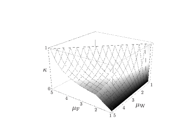
Figure 2: The demand index $\kappa$ as a function (24) of ${\mu_{\rm F}}$ and ${\mu_{\rm W}}$.

More generally, a function $(A-1)/(A-\delta)$ with $A>1$ has the required property, but by choosing $A=2$ we obtain $d\kappa/d\delta|_{\delta=1}=1$, so that $\kappa\simeq\delta$ for $\delta\rightarrow 1$. This proximity of $\kappa$ and $\delta$ is desirable to some extent as the data often shows $\delta$ in the range 0.5 to 1.

In summary, the superstatistics framework predicts that the Pareto indices ${\mu_{\rm W}}$ and ${\mu_{\rm F}}$ determines the Demand Index $\kappa$ as follows:

$$\kappa=\begin{cases}\displaystyle\frac{1}{{\mu_{\rm W}}-{\mu_{\rm F}}+1}&\mbox{for }2<{\mu_{\rm F}};\\[15.0pt] \displaystyle\frac{{\mu_{\rm F}}-1}{{\mu_{\rm W}}-1}&\mbox{for }1<{\mu_{\rm F}}<2.\end{cases}$$ (24)

This relation is illustrated in Fig.2.

III Empirical Facts

A Database and the Analysis

In calculating the productivity $c$ by Eq.(3) from data, we calculate the value added $Y$ by the method put forward by the Bank of Japan (Souma et al., 2009), which is the most common method used in Japan. As for the number of workers $L$, we use the average of the value of that year and that of the past year, as each are defined to be the value at the end of the year.

Figure 3: Total number of firms (left) and workers (right) in our database, both for manufacturing sector (dashed lines), nonmanufacturing sector (dotted lines) and both sectors (solid lines).

For comprehensive, high-accuracy study, we made a database from two sources:

Nikkei-NEEDS.

Nikkei Economic Electronic Databank System (NEEDS) database is a commercial product available from Nikkei Media Marketing, Inc. (2008) and contains financial data of all the listed firms in Japan. This is a well-established and representative database, widely used for various purposes from research to practical business applications. We have extracted data from their 2007 CD-ROM version, which contains two to three thousand firms and five to six million workers.

CRD.

Credit Risk Database (Credit Risc Database Association, 2008) is the first and only database for small-to-medium firms in Japan. It started collecting data from both banks and credit guarantee corporations (Credit Guarantee Corporations, 2008) since 2001. The latter, however, does not contain enough database entry necessary for the Bank-of-Japan method and thus are omitted from our database.

By combining these two database and removing any overlap, we have obtained a unified database that covers a wide range of firms in Japan. The total numbers of the firms and workers covered in this unified database is plotted in Fig.3.

Unfortunately, CRD data covers only from 1996 to 2006, and does no go far in the past, unlike Nikkei-NEEDS. This limits our unified database to the same short period. We, however, consider that it is important to include small-to-medium firms to our analysis so that we have a view of the whole spectrum of firms and workers in Japan. Thus we have decided to create and analyse this database. In coming years, we trust that CRD will keep collecting data. So, we may extend our analysis to future, if not past, by continuing and expanding what we have started here in this paper.

We need a model distribution to fit the data and extract the value of the Pareto indices. It has to have several properties: (i) It has be defined in the whole range, $c\in[0,\infty]$; (ii) it has to have power law (13) and (14) for large $c$; and (iii) it has to be able to describe the data to some accuracy over the whole region. The power law manifest itself as the straight line in the log-log rank-size plots of the data (see Fig.4.) Since its gradient is the Pareto index, its value is estimated fitting the straight section of the rank-size plot with a straight line. Although this can be done easily and is intuitive, it has several pitfalls: Often, the definition of “the straight section” is ad-hoc. Slight change of it can bring nonnegligible change in the value of the Pareto index. Even if a good one can be found for a particular year, it might not work for other years of the same database, which make comparison of different years meaningless.

The “Generalized Beta Distribution of the Second Kind” (GB2) (Kleiber and Kotz, 2004) satisfies the property (i)-(iii) and yet manageable. It is defined by the following pdf;

$$p^{\rm(GB2)}(c) =\frac{q}{B(\mu/q,\nu/q)}\frac{1}{c}\biggl{(}\frac{c}{c_{1}}\biggr{)}^{\nu}\left[\,1+\biggl{(}\frac{c}{c_{1}}\biggr{)}^{q}\right]^{-(\mu+\nu)/q},$$ (25)

where the four parameters satisfy constraints $\mu,\nu,q,c_{1}>0$. Since for large $c$;

$$p^{\rm(GB2)}(c)\simeq\biggl{(}\frac{c}{c_{1}}\biggr{)}^{-\mu-1},$$ (26)

the parameter $\mu$ is the Pareto index. Incidentally, its cumulative distribution functions (cdf) is the following:

$$P^{\rm(GB2)}_{>}(c):=\int_{c}^{\infty}p^{\rm(GB2)}(c)\,dc.=\frac{B(z,\mu/q,\nu/q)}{B(\mu/q,\nu/q)},\quad z=\left[\,1+\biggl{(}\frac{c}{c_{1}}\biggr{)}^{q}\right]^{-1},$$ (27)

where $B(z,s,t)$ is the incomplete Beta function with $B(1,s,t)=B(s,t)$. (Detailed study of small-to-medium productivity was done by Souma et al. (2009) using this GB2 distribution.)

B Manufacturing firms

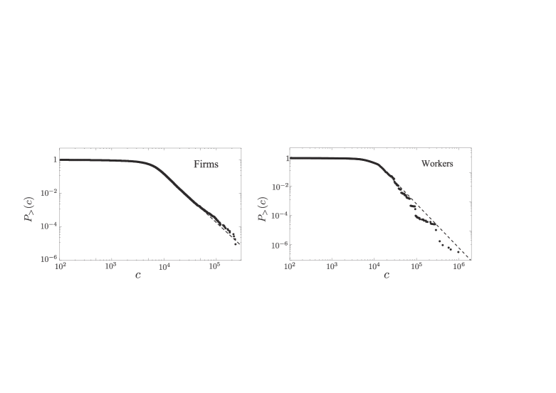
Figure 4: The rank-size plot of the productivity data (dots) and the best-fit cdf (dashed line) for firms (left) and workers (right) in 2004.

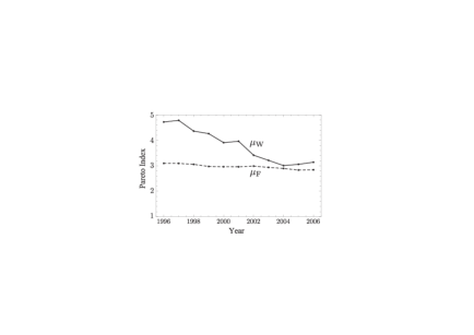
Figure 5: The Pareto indices ${\mu_{\rm F}}$ and ${\mu_{\rm W}}$ for the manufacturing sector.

The rank-size plots of the productivity of the manufacturing sector in 2004 is given in Fig.4 by dots, together with the best-fit cdf obtained by the maximum likelihood method. In these log-log plots, we see that the actual distributions of the data are close to straight lines for large $c$, which implies that it obeys the power law (i.e., the Pareto law) as we have discussed above. The best-fit cdf (dashed lines) indeed represents the data to good accuracy. The situation is quite similar in all other years.

The values of the Pareto indices ${\mu_{\rm F}}$ and ${\mu_{\rm W}}$ thus obtained are plotted in Fig.5. Substituting these values to Eq.(24), we have obtained the value of the demand index $\kappa$ joined by solid lines in Fig.6. We see here that the demand is slowing rising during this period, which is in agreement with general observations in Japan. Plotted in Fig.6 with dashed lines is the Nikkei Business Index (NBI), which is a major business index in Japan (Nikkei Net Interactive, 2008). We observe here that their correlation is good to some extent, which is consistent with the fact that our demand index $\kappa$ provides a measure of demand.

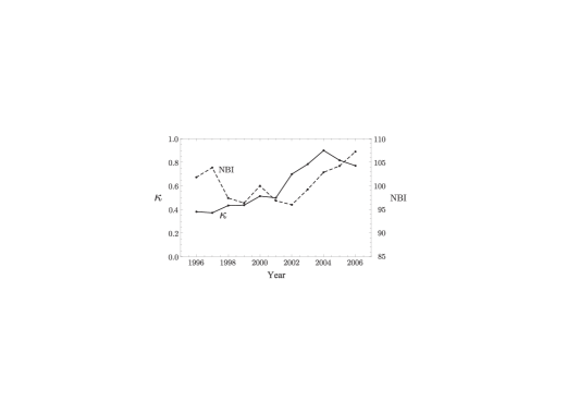
Figure 6: The demand index $\kappa$ for the manufacturing sector (solid lines) and the Nikkei Business Index (dashed lines).

C Nonmanufacturing (service) firms

In the nonmanufacturing sector, the same analysis leads to the result plotted in Fig.7. It is quite notable that it is completely different from the manufacturing sector: The Pareto index ${\mu_{\rm F}}$ is larger than ${\mu_{\rm W}}$. Since the larger Pareto index means that the pdf is damped highly for large $c$, this means that the higher productivity firms, more workers are employed. This is not allowed under the ordinary Boltzmann distribution (8) due to the Boltzmann factor $e^{-\beta c}$. It is not allowed in the superstatistics either, since it is an weighted average over the Boltzmann distribution. Therefore, this behaviour of the nonmanufacturing sector calls for extension of the theoretical framework.

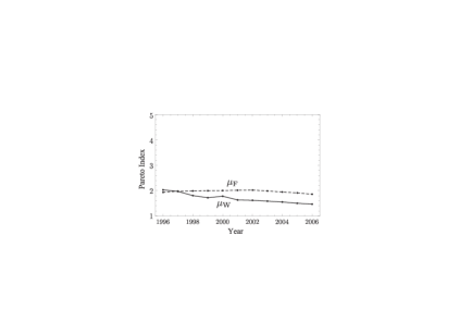
Figure 7: The Pareto indices ${\mu_{\rm F}}$ and ${\mu_{\rm W}}$ for the nonmanufacturing sector.

IV Productivity of Sectors

Productivity of sectors are of interest. Our database, following Nikkei NEEDS, contains 26 sectors, among which 15 are manufacturing sectors and 12 nonmanufacturing sectors. Their productivity distributions from 1996 to 2006 is plotted in Fig.8. Evident in this plot is that the productivity distribution obeys the power-law with the Pareto index $\mu\simeq 1.6$ every year. Since the number of data is limited, unlike the firms and workers, fitting with GB2 distribution and estimating the value of $\mu$ is not very illuminating. In other words, the obtained values of $\mu$ would suffer from large statistical errors. It is more so if manufacturing sectors and nonmanufacturing sectors are studied separately.

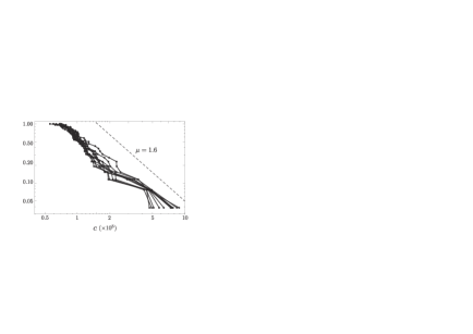
Figure 8: Productivity distribution of 26 sectors from 1996 to 2006. The dashed line is a power-law distribution with the Pareto index $\mu=1.6$.

The notable feature of the sector distribution is the (i) it is approximately Pareto and (ii) the values of the Pareto index are certainly lower than that of firms every year. This is in accordance with the idea of applying superstatistics framework to firms and sectors, in contrast to workers and firms (Aoyama et al., 2008b): We may now think of a firm (instead of a worker) choosing a sector (instead of a firm) for its business activity. Applying the superstatistics to them, we find again that the Pareto index of the firms are higher than that of sectors. This is what we observe in Fig.8.

V Conclusion and Discussions

We have studied the superstatistics theory of productivity and have proposed the demand index $\kappa$, which determines the relation between the Pareto indices of the productivity distributions of firms and workers. Analysis of the whole spectrum, from small to large, firms in Japan from 1996 to 2006 is carried out and manufacturing sector was studied within the superstatistics framework.

One might argue that what we have been observing is a temporal situation and eventually, the effect of shocks, including 1999 bubble collapse, would be averaged out and the productivity starts converging to a unique value, as predicted by the orthodox equilibrium theory. In order to study this point, we have examined the change of the productivity of sectors over the years. The result is plotted in Fig.9. Each line represents a sector, solid lines for manufacturing and dashed lines for nonmanufacturing. In this Figure, we see that they are far from arriving at a unique value. Rather, they keeps fluctuating. Sometimes, the difference of productivity between the sectors widens. This sort of behaviour is typical in physical systems. The distribution is maintained, while viewed in detail, each atoms keeps changing its energy and momentum. Such is the nature of physical equilibrium and so is the economic system.

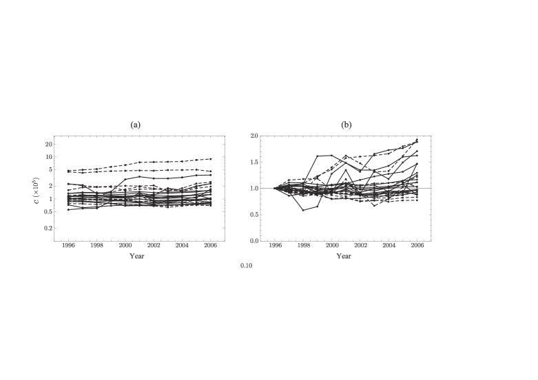
Figure 9: Evolution of productivity of each sector. sectors. (a) is the actual value, while (b) is the value normalized at 1996. Solid lines are of manufacturing sectors and dashed lines are of nonmanufacturing sectors.

We stress here that the distribution (20) of the demand $D$ is unique in the superstatistics framework: It has to obey this distribution if Pareto law hold for both firms and workers and Eq. (18) is satisfied. Just what kind of dynamics and economic principles underlies the demand distribution (20) is unknown. It would be quite interesting and important to construct a model which leads to this kind of behaviour. It is quite possible that such a model could be one of the building blocks useful and necessary for reconstructing macro-economics.

On the other hand, nonmanufacturing (service) sector showed peculiar characteristics that has never been seen before. The Pareto index for the workers were larger than that for firms.

In the ordinary Boltzmann distribution (10), the positivity of the temperature guarantees that higher the productivity less workers are employed. Since superstatistics is the weighted average of the Boltzmann distribution, no matter what the weight function $f_{\beta}(\beta)$ is, the higher productively means less workers, which is the reason for ${\mu_{\rm F}}<{\mu_{\rm W}}$. The fact that the nonmanufacturing sector violates this constraint means that the weighted average over the negative temperature is required.

Negative temperature is possible for a physical system in nonequilibrium. One such an example is a laser, where many atoms or electrons are in a excited state before the emission. For the current case, there is at least one economic reason why it is required; excess of the demand. There are certain limits to the productivity of a given firm due to many constraints it faces. But by hiring more people while maintaining the same structure, firms can increase its add value, thereby meeting the increasing demand. Just such cold be happening in the nonmanufacturing industry.

On the other hand, superstatistics of the negative temperature has not been developed yet: While it is easy to expand the weighted average over the negative temperature, its full consequences are not clear at this stage. It would therefore be quite interesting to develop this theory and use it to deal with the nonmanufacturing sector.

Appendix: Temperature and the Demand

We first note the following three basic properties (i)–(iii).

1. The temperature, $T=1/\beta$ is a monotonically increasing function of the aggregate demand, $D$. We can prove it using Eq.(7) as follows:

   $$\frac{dD}{dT}=-\frac{1}{T^{2}}\frac{dD}{d\beta}=\beta^{2}\frac{d^{2}}{d\beta^{2}}\ln Z(\beta)=\beta^{2}\left(\langle c^{2}\rangle_{\beta}-\langle c\rangle_{\beta}^{2}\right)\geq 0,$$ (28)

   where $\langle c^{n}\rangle_{\beta}$ is the $n$-th moment of productivity defined as follows:

   $$\langle c^{n}\rangle_{\beta}\equiv\frac{1}{Z(\beta)}\int_{0}^{\infty}c^{n}p^{(\rm F)}(c)\,e^{-\beta c}\,dc.$$ (29)

   Note that $\langle c\rangle_{\beta}=D$. This is a natural result. As the aggregate demand $D$ rises, workers move to firms with higher productivity. It corresponds to the higher temperature due to the weight factor $e^{-\beta c}$.

2. For $T\rightarrow 0$ ($\beta\rightarrow\infty$),

   $$D\rightarrow 0.$$ (30)

   This is evident from the fact that in the same limit the integration in Eq.(9) is dominated by $c\simeq 0$ due to the factor $e^{-\beta c}$.

3. For $T\rightarrow\infty$ ($\beta\rightarrow 0$),

   $$D\rightarrow\int_{0}^{\infty}c\,p^{(\rm F)}(c)\,dc\ (=\langle c\rangle_{0}).$$ (31)

   This can be established based on the property (i) because $D=\langle c\rangle_{\beta}\rightarrow\langle c\rangle_{0}$ as $\beta\rightarrow 0$ and $Z(0)=1$.

Let us now study the small $\beta$ (high temperature) properties. One possible approximation for Eq.(9) is obtained by expanding the factor $e^{-\beta c}=1-\beta c+\cdots$ and carrying out the $c$-integration in each term. This leads to the following:

$$Z(\beta) =\int_{0}^{\infty}p^{(\rm F)}(c)\left(1-\beta c+\frac{1}{2}(\beta c)^{2}+\dots\right)dc$$

$$=1-\langle c\rangle_{0}\beta+\frac{1}{2}\langle c^{2}\rangle_{0}\beta^{2}+\dots,$$ (32)

where we have used the normalization condition,

$$\int_{0}^{\infty}p^{(\rm F)}(c)\,dc=1.$$ (33)

The result (32) is, however, valid only for ${\mu_{\rm F}}>2$ since $\langle c^{2}\rangle_{0}$ is infinite for ${\mu_{\rm F}}\leq 2$, which is true as we have seen.

The correct expansion for $1<{\mu_{\rm F}}<2$ is done in the following way. We first separate out the first two terms in the expansion of the factor $e^{-\beta c}$;

$$Z(\beta) =\int_{0}^{\infty}p^{(\rm F)}(c)\left(1-\beta c+(e^{-\beta c}-1+\beta c)\right)dc$$

$$=1-\langle c\rangle_{0}\beta+Z_{2}(\beta),$$ (34)

$$Z_{2}(\beta) \equiv\int_{0}^{\infty}p^{(\rm F)}(c)\,g(c)dc=\int_{0}^{\infty}\left(-\frac{\partial}{\partial c}P^{(\rm F)}_{>}(c)\right)g(c)dc$$

$$=\int_{0}^{\infty}P^{(\rm F)}_{>}(c)\frac{\partial g(c)}{\partial c}dc,$$ (35)

where $g(c)=e^{-\beta c}-1+\beta c$ is a monotonically increasing function of $c$ with

$$g(0)=g^{\prime}(0)=0.$$ (36)

The $c$-integration in Eq.(35) is dominated by the asymptotic region of $c$ for small $\beta$. Therefore, the leading term in $Z_{2}(\beta)$ is evaluated by substituting the asymptotic expression of $p^{(\rm F)}(c)$;

$$P^{(\rm F)}_{>}(c)\simeq\left(\frac{c}{c_{0}}\right)^{-{\mu_{\rm F}}},$$ (37)

into Eq.(35). We thus arrive at the following:

$$Z_{2}(\beta) =\int_{0}^{\infty}\left(\frac{c}{c_{0}}\right)^{-{\mu_{\rm F}}}\frac{\partial g(c)}{\partial c}dc+\cdots$$

$$={\mu_{\rm F}}\Gamma(-{\mu_{\rm F}})(c_{0}\beta)^{\mu_{\rm F}}+\cdots.$$ (38)

The case ${\mu_{\rm F}}=2$ can be obtained by taking the limit ${\mu_{\rm F}}\rightarrow 2+$ in the following expansion valid for $2<{\mu_{\rm F}}<3$:

$$Z(\beta)=1-\langle c\rangle_{0}\beta+\frac{1}{2}(\langle c^{2}\rangle_{0}-\langle c\rangle_{0}^{2})\beta^{2}+{\mu_{\rm F}}\Gamma(-{\mu_{\rm F}})(c_{0}\beta)^{\mu_{\rm F}}+\dots.$$ (39)

which can be obtained in the manner similar to the above. The third term is finite for ${\mu_{\rm F}}>2$, but diverges as ${\mu_{\rm F}}\rightarrow 2+$ as

$$\langle c^{2}\rangle_{0}\rightarrow\frac{2c_{0}^{2}}{{\mu_{\rm F}}-2}.$$ (40)

This cancels the divergence of the fourth term in the same limit and the remaining leading term is as follows:

$$Z(\beta)=1-\langle c\rangle_{0}\beta-(c_{0}\beta)^{2}\log(c_{0}\beta)+\dots.$$ (41)

In summary, the partition function behaves as follows:

$$Z(\beta)=\begin{cases}1-\langle c\rangle_{0}\beta+\frac{1}{2}\langle c^{2}\rangle_{0}\beta^{2}+\dots&\mbox{for }2<{\mu_{\rm F}};\\ 1-\langle c\rangle_{0}\beta-(c_{0}\beta)^{2}\log(c_{0}\beta)+\dots&\mbox{for }{\mu_{\rm F}}=2;\\ 1-\langle c\rangle_{0}\beta+{\mu_{\rm F}}\Gamma(-{\mu_{\rm F}})(c_{0}\beta)^{\mu_{\rm F}}+\dots&\mbox{for }1<{\mu_{\rm F}}<2.\\ \end{cases}$$ (42)

Substituting the above in Eq.(7), we obtain the following:

$$D=\begin{cases}\langle c\rangle_{0}-\left(\langle c^{2}\rangle_{0}-\langle c\rangle_{0}^{2}\right)\beta+\dots.&\mbox{for }2<{\mu_{\rm F}};\\ \langle c\rangle_{0}+2c_{0}^{2}\beta\log(c_{0}\beta)+\dots&\mbox{for }{\mu_{\rm F}}=2;\\ \langle c\rangle_{0}-{\mu_{\rm F}}^{2}\Gamma(-{\mu_{\rm F}})c_{0}^{\mu_{\rm F}}\beta^{{\mu_{\rm F}}-1}+\dots&\mbox{for }1<{\mu_{\rm F}}<2.\\ \end{cases}$$ (43)

References

- (1)
- Aoki and Yoshikawa (2007) Aoki, M. and H. Yoshikawa, Reconstructing Macroeconomics – A Perspective from Statistical Physics and Combinatorial Stochastic Processes, Cambridge, U.K.: Cambridge University Press, 2007.
- Aoyama et al. (2008a) Aoyama, H., H. Yoshikawa, H. Iyetomi, and Y. Fujiwara, “Labour Productivity Superstatistics,” arXiv:0809.3541, 2008. To appear in Progress of Theoretical Physics: Supplement (Yukawa Institute, Kyoto, Japan, 2009).
- Aoyama et al. (2008b) , , , and , “Productivity Dispersion: Fact, Theory and Implications,” arXiv:0805.2792, RIETI discussion paper 08-E-035, 2008.
- Ausloos and Lambiotte (2006) Ausloos, M. and R. Lambiotte, “Brownian particle having a fluctuating mass,” Physical Review E, 2006, 73 (1), 11105.
- Beck (2005) Beck, C., “Superstatistics: Recent developments and applications,” 2005. arXiv:cond-mat/0502306v1.
- Beck (2008) , “Recent developments in superstatistics,” arXiv:0811.4363v1, 2008.
- Beck and Cohen (2003) and E. G. D. Cohen, “Superstatistics,” Physica A, 2003, 322, 267.
- Credit Guarantee Corporations (2008) Credit Guarantee Corporations, www.zenshinhoren.or.jp/file/epamph.pdf 2008.
- Credit Risc Database Association (2008) Credit Risc Database Association, www.crd-office.net/CRD/english/index.htm 2008.
- Ikeda and Souma (2008) Ikeda, Y. and W. Souma, “International Comparison of Labor Productivity Distribution for Manufacturing and Non-Manufacturing Firms,” arXiv:0812.0208v4, 2008. To appear in Progress of Theoretical Physics: Supplement (Yukawa Institute, Kyoto, Japan, 2009).
- Kleiber and Kotz (2004) Kleiber, C. and Samuel Kotz, Statistical Size Distributions in Economics and Actuarial Sciences, Hoboken, New Jersey: John Wiley and Sons, Inc., 2004.
- Luczka and Zaborek (2004) Luczka, J. and B. Zaborek, “Brownian motion: a case of temperature fluctuations,” Arxiv preprint cond-mat/0406708, 2004.
- Nikkei Media Marketing, Inc. (2008) Nikkei Media Marketing, Inc., www.nikkeimm.co.jp/english/index.html 2008.
- Nikkei Net Interactive (2008) Nikkei Net Interactive, http://www.nni.nikkei.co.jp/ 2008.
- Pareto (1896) Pareto, Vilfredo, Cours d’économie politique 1896.
- Souma et al. (2009) Souma, W., Y. Ikeda, H. Iyetomi, and Y. Fujiwara, “Distribution of Labour Productivity in Japan over the Period 1996-2006,” Economics (to appear in this volume), 2009.
- Yoshikawa (2003) Yoshikawa, H., “The Role of Demand in Macroeconomics,” The Japanese Economic Review, 2003, 54, 1.