Quantum Hall effect in a high-mobility two-dimensional electron gas
on the surface of a cylinder

Abstract

The quantum Hall effect is investigated in a high-mobility two-dimensional electron gas on the surface of a cylinder. The novel topology leads to a spatially varying filling factor along the current path. The resulting inhomogeneous current-density distribution gives rise to additional features in the magneto-transport, such as resistance asymmetry and modified longitudinal resistances. We experimentally demonstrate that the asymmetry relations satisfied in the integer filling factor regime are valid also in the transition regime to non-integer filling factors, thereby suggesting a more general form of these asymmetry relations. A model is developed based on the screening theory of the integer quantum Hall effect that allows the self-consistent calculation of the local electron density and thereby the local current density including the current along incompressible stripes. The model, which also includes the so-called ‘static skin effect’ to account for the current density distribution in the compressible regions, is capable of explaining the main experimental observations. Due to the existence of an incompressible-compressible transition in the bulk, the system behaves always metal-like in contrast to the conventional Landauer-Büttiker description, in which the bulk remains completely insulating throughout the quantized Hall plateau regime.

I Introduction

The self-rolling of thin pseudomorphically strained semiconductor bilayer systems based on epitaxial heterojunctions grown by molecular-beam epitaxy (MBE) as proposed by Prinz and coworkers Prinz allows to investigate physical properties of systems with nontrivial topology. Using a specific heterojunction, where the high-mobility two-dimensional electron gas (2DEG) in a 13nm-wide GaAs single quantum well could be effectively protected from charged surface states, the electron mobility in the quantum well remains high even after fabrication of freestanding layers Friedland0 and particularly in semiconductor tubes. FriedlandI ; VorobevI Implementing this new design, the low-temperature mean free path of electrons $l_{S}$ can be kept long, comparable to the curvature radius $r$ of the tube, opening the way to investigate curvature-related adiabatic motion of electrons on a cylindrical surface, such as ‘trochoid’- or ‘snake’-like trajectories. FriedlandI ; FriedlandII

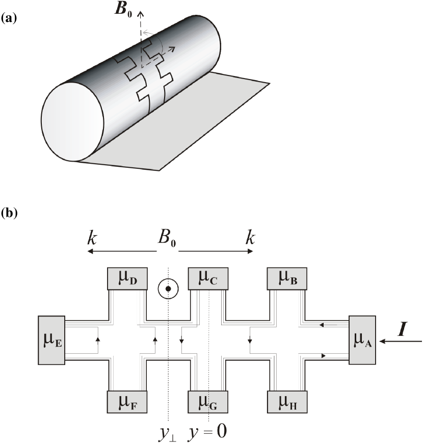
Figure 1: (a) Sketch of a Hall-bar on the periphery of a cylinder. (b) Schematic of such a Hall bar indicating the gradient of the magnetic field $k$, the imposed current $I_{\rm EA}$ and imposed chemical potentials $\mu_{i}$ at leads $i$. The magnetic field is perpendicular at the position $y_{\perp}$ ($y=0$ is defined to be at the center Hall leads $C-G$). The 1DLS are shown schematically. The arrows indicate their chirality .

Placing a tube with a high mobility 2DEG in a static and homogeneous magnetic field $\textbf{B}_{0}$, the fundamental dominant modification is the gradual change of the component of the magnetic field perpendicular to the surface $B_{\perp}$ along the periphery of the tube, which is equivalent to a gradual change of the filling factor $\nu$. This is an important modification for the quantum Hall effect, which has recently stimulated notable theoretical interest. Karasev ; Ferrari

Earlier investigations of the magneto-transport with spatially varying magnetic fields, created by a density gradient Ponomarenko or by magnetic field barriers inclined with respect to the substrate facets Ibrahim , demonstrated that the spatial current-density distribution is modified, thereby creating striking lateral electric field asymmetries. Similarly, in wave guides on cylindrical surfaces the chemical potential differences measured along opposite edges of the Hall bar and with opposite magnetic field directions was shown to differ by a factor of 1000 or even to reverse its sign. VorobevI ; FriedlandII

This large resistance anisotropy, which even persists at higher magnetic fields, was intuitively explained by the so-called bending away of one-dimensional Landau-states (1DLS) from the edges into the bulk MendachI ; VorobevI , as demonstrated in Fig. 1(b). Figure 1 shows schematically a Hall bar structure oriented along the periphery of a cylinder as used for our investigation. A current $I_{\rm EA}$ is imposed between the current leads ${E-A}$, which therefore flows parallel to the gradient $k=\delta B_{\perp}/\delta y$ and imposes the chemical potentials $\mu_{i}$ at terminals i. By adopting the Landauer-Büttiker formalism the longitudinal resistances can be calculated for integer filling factors $\nu=hn(2eB)^{-1}=1,2,3...$ as follows:

$$\begin{split}R^{L}_{\rm DC}=~{}&\frac{\mu_{D}-\mu_{C}}{I_{\rm EA}}=\frac{h}{2e^{2}}(\frac{1}{\nu_{0}}-\frac{1}{\nu_{\rm DF}})=R^{H}_{0}-R^{H}_{\rm DF}\\ R^{L}_{\rm FG}=~{}&\frac{\mu_{F}-\mu_{G}}{I_{\rm EA}}=\frac{h}{2e^{2}}(\frac{1}{\nu_{0}}-\frac{1}{\nu_{\rm CG}})=R^{H}_{0}-R^{H}_{\rm CG}\\ \end{split}$$ (1)

Here, the position $y_{\perp}$ at which the magnetic field $\textbf{B}_{0}$ is directed along the normal to the surface n, is located between the leads ${F-G}$ and ${D-C}$. $\nu_{0}$, $\nu_{\rm ij}$ are filling factors at the positions $y_{\perp}$ and of the Hall lead pairs $i-j$, respectively. $h$ denotes Planck’s constant and $e$ the electronic charge. For clarity, we use the superscripts $L$ and $H$ for the longitudinal and Hall resistances, respectively. The arrows in Fig. 1 indicate the chirality of the 1DLS and determine those Hall leads, from which the potential is induced into the opposite longitudinal lead pair for a given direction of the magnetic field. For the situation in Fig. 1, the Hall resistance $R^{H}_{\rm DF}$ induces a finite $R^{L}_{\rm DC}$, while the Hall voltage $R^{H}_{\rm CG}$ do so for $R^{L}_{\rm FG}$, etc.

The longitudinal resistances for pairs of leads outside the position $y_{\perp}$ read:

$$\begin{split}R^{L}_{\rm CB}=~{}&\frac{\mu_{C}-\mu_{B}}{I_{\rm EA}}=0\\ R^{L}_{\rm GH}=~{}&\frac{\mu_{G}-\mu_{H}}{I_{\rm EA}}=\frac{h}{2e^{2}}(\frac{1}{\nu_{\rm CG}}-\frac{1}{\nu_{\rm BH}})=R^{H}_{\rm CG}-R^{H}_{\rm BH}.\end{split}$$ (2)

Reversing the direction of the magnetic field results in an interchange of $R^{L}_{\rm DC}\rightleftharpoons R^{L}_{\rm FG}$ and $R^{L}_{\rm CB}\rightleftharpoons R^{L}_{\rm GH}$ .

The resistance anisotropy in Hall bars with magnetic field gradient along the current direction is also well known from classical (metal-like) electron transport studies at low magnetic fields. The anisotropy was also predicted by Chaplik, and is referred to as the ‘static skin effect’ (SSE). Chaplik ; MendachI An experimental demonstration was reported by Mendach and coworkers. MendachII The physical origin of this effect is the gradual change of the Hall field along the Hall bar which acts on the longitudinal electric field so that it becomes different on both sides of the Hall bar. Microscopically, the SSE is a result of an exponential current-squeezing towards one of the Hall bar edges and is characterized by the skin length $L_{\rm skin}=(\emph{k}\mu)^{-1}$, where $\mu$ is the carrier mobility. Asymptotically, for high magnetic fields the SSE is described by the same Eq. (2), in the form of: $R^{L}_{\rm CB}=0$, $R^{L}_{\rm BH}=R^{H}_{\rm CG}-R^{H}_{\rm BH}$.

Despite this similarity, both mechanisms differ antagonistically in their microscopically origin. For the explanation of the SSE it is assumed that a current flows exclusively at one edge of the Hall bar which changes to the opposite one by inverting the magnetic field direction. In contrast, the application of the Landauer-Büttiker formalism for the 1DLS states presupposes current flow at both edges of the Hall bar. In the quantum Hall regime, for the situation presented in Fig. 1, the longitudinal resistance $R^{L}_{\rm CB}$ with leads, which are still bound by the outermost edge channels, remains zero at all times. In contrast, the bending of the innermost 1DLS channels into the opposite leads causes the nonzero longitudinal resistance $R^{L}_{\rm GH}$ that compensates the change of the transverse Hall-voltages.

In this paper, we present quantum Hall effect measurements of a high- mobility 2DEG on a cylinder surface and show that a significant part of the results cannot be explained by the simplified 1DLS-approach. We observe clear indications that the actual current-density distribution in the Hall bar should be reconsidered and propose a new model which takes into account more precisely the sequential current flow along incompressible stripes and metal-like compressible regions, for which a current distribution according to the SSE should be considered.

II Experimental

The layer stack, with an overall thickness of 192 nm including the high mobility 2DEG, was grown on top of a 20nm-thick $\rm In_{\rm 0.15}Ga_{\rm 0.85}As$ stressor layer, an essential component of the strained multi-layered films (SMLF). An additional 50nm-thick AlAs sacrificial layer is introduced below the SMLF in order to separate the SMLF from the substrate.

For the fabrication of curved 2DEGs, we first fabricate conventional Hall bar structures in the planar heterojunction along the $[100]$ crystal direction. The two 20 $\mu$m-wide Hall bar arms and three opposite 4$\mu$m-narrow lead pairs, separated by 10 $\mu$m, are connected to Ohmic contact pads outside of the rolling area in a similar manner as the recently developed technology to fabricate laterally structured and rolled up 2DEGs with Ohmic contacts.VorobevII ; MendachIII Subsequently, the SMLF including the Hall bar was released by selective etching away of the sacrificial AlAs layer with a $5\%$ HF acid/water solution at 4 ^∘C starting from a $[010]$ edge. In order to relax the strain, the SMLF rolls up along the $[100]$ direction forming a complete tube with a radius $r$ of about 20 $\mu$m. We report on specific structures which are described in Ref. FriedlandI, and which have a carrier density of $n\cong(6.8-7.2)\times$10¹⁵ m^-2 and a mobility of up to 90 m²(Vs)^-1 along the $[100]$ crystal direction before and after rolling-up. All presented measurements were carried out at a temperature $T$= 100 mK.

III Results and discussion

III.1 Asymmetry of the longitudinal resistances

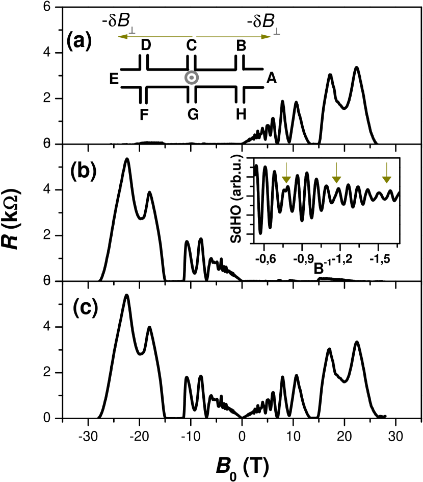
Figure 2: Longitudinal resistances with a magnetic field $B_{0}$ normal to the surface at the center Hall-leads $y_{\perp}=0$. (a) $R^{L}_{\rm DC}$, the inset shows the orientation of the Hall-bar, (b) $R^{L}_{\rm CB}$, the inset shows the second derivative of $R^{L}_{\rm CB}$, as a function of the reciprocal of the magnetic field, (c) $R^{L}_{\rm DB}$.

The strong asymmetry of the longitudinal resistances for the current parallel to the magnetic field gradient $k$ is demonstrated in Fig. 2. The magnetic field is perpendicular to the surface around the center Hall lead pair $C-G$ the position of which we define as $y_{\perp}=0$. The longitudinal resistances $R^{L}_{\rm CB}$ - on the right side and $R^{L}_{\rm DC}$ - on the left side of this position differ strongly for a given magnetic field and are asymmetric with respect to the direction of the magnetic field. For example, at a magnetic field of $B_{0}$ = 0.66 T, where $R^{L}_{\rm CB}$ shows a minimum, the ratio $R^{L}_{\rm DC}/R^{L}_{CB}$ exceeds 300. With the deviation $\delta y$ towards either side of the perpendicular field position, the component of the magnetic field decreases as $\emph{B}_{\rm\perp}=\emph{B}_{0}$cos$(\varphi_{\delta y})$, where $\varphi_{\delta y}$ = arcsin$(\delta y/r)$. Accordingly, the magnetic field gradient can be calculated as $k\cong B_{0}\delta y/r^{2}$. When we consider the given mobility and the field value $B_{0}$ = 0.66 T, we can estimate a skin length $L_{\rm skin}\cong 670~{}nm$ at the positions of the next left and right pairs of the Hall leads. As the direction of current squeezing is determined by the sign of the field gradient, we find that for positive magnetic field values, that the current is concentrated exponentially close to the upper Hall bar edge between the $D-C$ leads, while the current is concentrated exponentially close to the lower Hall bar edge between the $G-H$ leads. Inverting the magnetic field direction results in a change of the Hall bar edges for the current flow.

In contrast, as can be seen in Fig. 2(c), the longitudinal resistances measured between leads $D$ and $B$ is nearly symmetric, despite the fact that $R^{L}_{\rm DB}$ results from current flow in different spatial areas.

III.2 Shubnikov de Haas oscillations

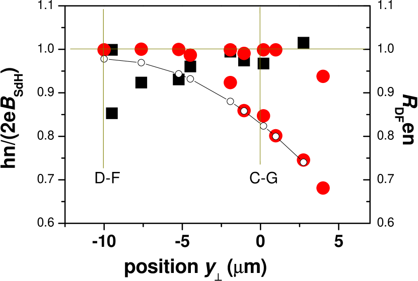
Figure 3: Fundamental frequency Shubnikov de Haas oscillation $B_{\rm SdH}^{-1}$ in units of $2e(hn)^{-1}$ calculated from $R^{L}_{\rm DC}$ (closed circles) and $R^{L}_{\rm FG}$ (closed squares). The low field Hall resistance $R^{H}_{\rm DF}$ in units of $(en)^{-1}$ is shown by is small open circles.

We observe a complex structure of the Shubnikov de Haas oscillations (SdHO). In particular, a clear beating in the SdHO results in nodes in the second derivative of the longitudinal resistances with respect to the inverse magnetic field as seen, for example, in the inset of Fig. 2(b). As a result, the low-field SdHO are composed of at least two fundamental SdHO frequencies $B_{\rm SdH}^{-1}$, as calculated by a Fourier transform analysis.

We have analyzed the two-frequency SdHO pattern by rotating the tube around the cylinder axis through an angle $\varphi$, thereby shifting the position $y_{\perp}$ away from the center pair of Hall leads $C-G$. For $y_{\perp}$ values between the longitudinal voltage leads $D-C$, Fig. 3 shows the dimensionless value $hn/(2eB_{\rm SdH})$ as a function of $y_{\perp}$. In the same figure, we present also the data for the classical Hall effect $R^{H}_{\rm DF}en$, which corresponds nicely to the lower frequency SdHO branch. Therefore, we conclude that this branch arises from the $B_{\perp}$ values at the pair of Hall leads $D-F$, which induce a voltage at the leads $D-C$. The upper branch, close to $hn/(2eB_{\rm SdH})=1$, reflects the SdHO for $B_{0}$ at the positions $y_{\perp}$. We conclude, therefore, that the two-frequency SdHO pattern is in accordance with Eq. (1) in the form of $R^{L}_{\rm DC}=R^{H}_{0}-R^{H}_{\rm DF},R^{L}_{\rm FG}=R^{H}_{0}-R^{H}_{\rm CG}$ as the SdHO of the corresponding longitudinal resistances reflects the filling factors values $\nu_{0}$ and $\nu_{\rm ij}$ at $y_{\bot}$ and the corresponding pair of Hall leads $i-j$, respectively.

III.3 Quantum Hall effect

The quantum Hall effect can be observed for a wide range of magnetic field gradients. Figure 4 shows the Hall resistances $R^{H}_{\rm BH}$ and $R^{H}_{\rm CG}$ and the longitudinal resistance $R^{L}_{\rm GH}$ for $y_{\perp}~{}=-9.4~{}\mu$m (close to the pair of Hall leads $D-F$), which represents a large gradient case. The filling factors differ substantially for subsequent Hall leads. For positive magnetic field values, the longitudinal resistances $R^{L}_{\rm DC}$ and $R^{L}_{\rm GH}$ are always non zero. As a special case, we indicate in Fig. 4 some of the magnetic field regions where both Hall terminals are at different but integer filling factors, thus proving the existence of quantized conductance in the non-zero longitudinal resistance $R_{\rm GH}$ in accordance with Eq. (2). Moreover, in Fig. 4, it can be seen that the equation $R^{L}_{\rm GH}=R^{H}_{\rm CG}-R^{H}_{\rm BH}$ holds for all positive magnetic fields values, i.e. also for non-integer filling factors, which is not guarantied by the Landauer-Büttiker approach for Eq. (2), but is in agreement with the local Kirchhoff’s law of voltage distribution in electronic circuits with current.

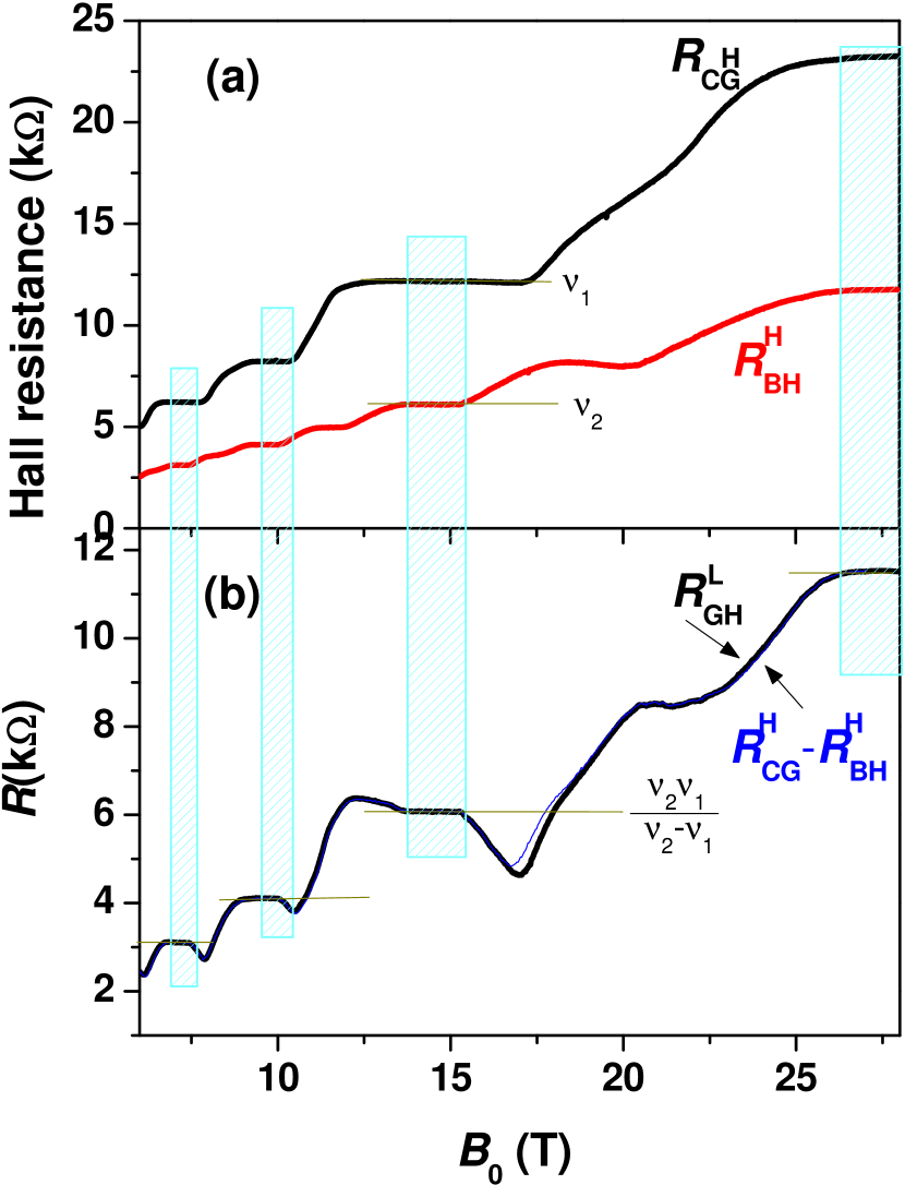
Figure 4: (a) Hall resistances $R^{H}_{\rm CG}$ and $R^{H}_{\rm BH}$, (b) longitudinal resistance $R^{L}_{\rm GH}$ for $y_{\perp}$= - 9.4 $\mu$ vs.$B_{\rm 0}$. Quantization in $R^{L}_{\rm GH}$ at $\nu_{2}\nu_{1}/(\nu_{2}-\nu_{1})$ is indicated by the shaded rectangles for those regions where $R^{H}_{\rm CG}$ and $R^{H}_{\rm BH}$ are at integer filling factors. We plot the calculated resistance $R^{H}_{\rm CG}$ - $R^{H}_{\rm BH}$ by a thin blue line.

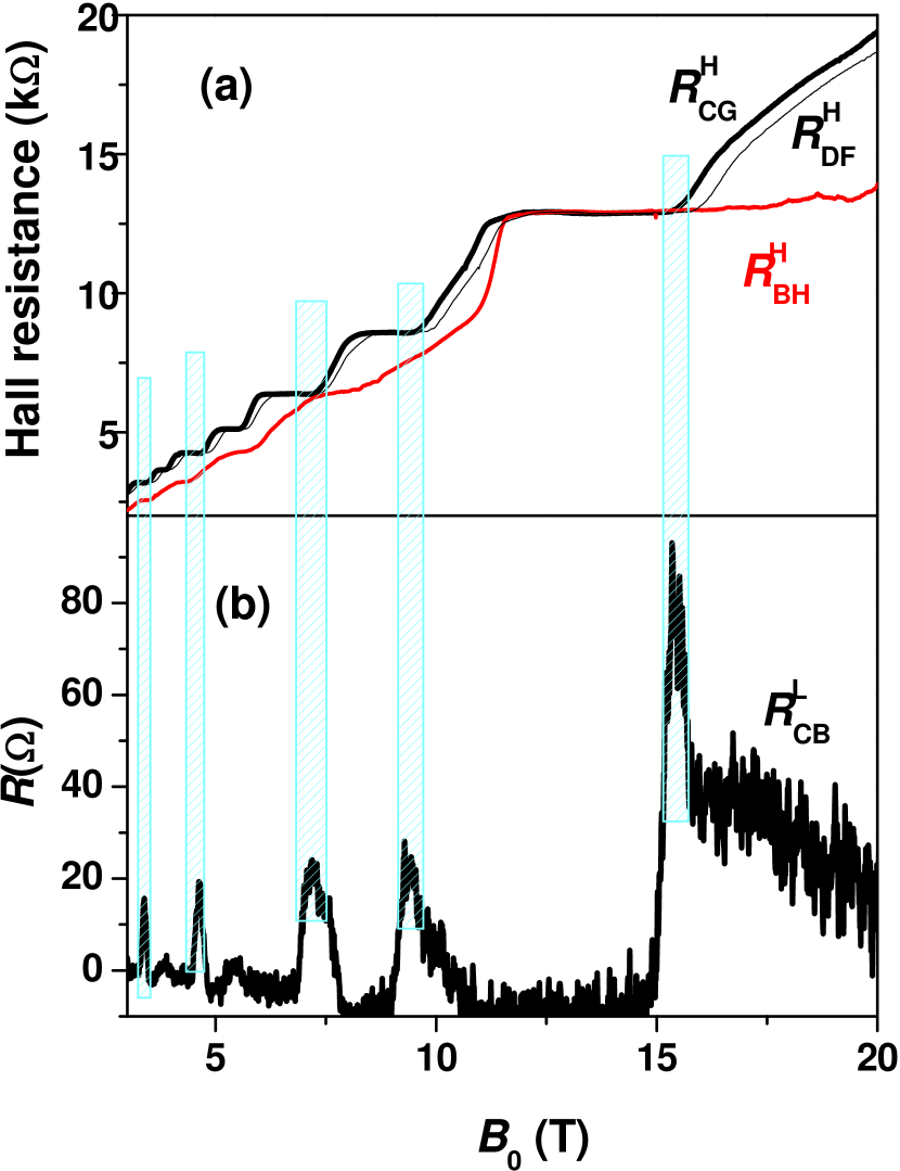
Figure 5: (a) Hall resistances $R^{H}_{\rm CG}$, $R^{H}_{\rm DF}$ and $R^{H}_{\rm BH}$, (b) longitudinal resistance $R^{L}_{\rm CB}$ for $y_{\perp}$=-2.1 $\mu$m vs. $B_{\rm 0}$. Peaks in $R^{L}_{\rm CB}$ appear at the nearest Hall lead pair at the high magnetic field end of the quantized Hall plateau.

Therefore, we conclude that for the large gradient case the equality between the outer left and outer right expressions in Eqs. (1) and (2) account for the current and voltage distribution in our system in a more general fashion than the simplified Landauer-Büttiker approach for conductance along one-dimensional channels. We will show that our model can be used for a more quantitative explanation.

In the case of moderate gradients, i.e. small distances of $y_{\perp}$ from the corresponding middle pair of Hall leads, we observe a striking deviation from the set of Eq. (2). Despite the fact that we should expect $R^{L}_{\rm CB}$=0 for any field value, we observe clear resistance maxima, which even increase in height with increasing magnetic field at the high magnetic field end of the quantized Hall plateau measured for the nearest pair of Hall leads, see Fig. 5. While the maximum values in $R^{L}_{\rm CB}$ remain an order of magnitude lower then the reverse one, namely $R^{L}_{\rm GH}$, they exceed the background minima due to the SSE at low magnetic fields by an order of magnitude. We exclude that these resistance maxima arise from a certain inaccuracy in the lead fabrication process, which could result in a small cross talk from the voltage inducing Hall lead pair $D-F$ into the lead C, by ensuring that the Hall resistance $R^{H}_{\rm DF}$ remains quantized at corresponding magnetic fields, see Fig. 5. In order to explain this effect, we will use our model as discussed in the following section.

IV Model

We now discuss our experimental findings in the light of self-consistent calculations of the density distribution. We exploit the inherent similarity of the filling factor gradient generated by the inhomogeneous magnetic field to the density gradient and utilize current confinement to one of the Hall bar edges resulting from the SSE. In our model calculations, we assume periodic boundary conditions in two dimensions to describe the Hall bar electrostatically. The magnetic field gradient is simulated by an electron density gradient, which essentially models the filling factor distribution over the Hall bar. The density gradient is generated by an external potential preserving the boundary conditions. The total electrostatic potential energy experienced by a spinless electron is given by

$$V_{\rm tot}(x,y)=V_{\rm bg}(x,y)+V_{\rm ext}(x,y)+V_{\rm H}(x,y),$$ (3)

where $V_{\rm bg}(x,y)$ is the background potential generated by the donors, $V_{\rm ext}(x,y)$ is the external potential resulting from the gates (which will be used to simulate the filling factor gradient) and the mutual electron-electron interaction is described by the Hartree potential $V_{\rm H}(x,y)$. We assume that this total potential varies slowly over the quantum mechanical length scale, given by the magnetic length $l_{b}=\sqrt{\hbar/m\omega_{c}}$ so that the electron density can be calculated within the Thomas-Fermi approximation in 2D SiddikiMarquardt ; Siddiki08:125423 according to

$$n_{\rm el}(x,y)=\int D(E,x,y)f(E+V_{\rm tot}(x,y)-\mu^{*})dE$$ (4)

where $D(E,x,y)$ is the (local) density of states, $f(E)=1/[\exp(E/k_{b}T)+1]$ the Fermi function, $\mu^{*}$ the electrochemical potential (which is constant in equilibrium), $k_{B}$ Boltzmann’s constant, and $T$ the temperature. Since the Hartree potential explicitly depends on the electron density via

$$V_{\rm H}(x,y)=\frac{2e^{2}}{\bar{\kappa}}\int_{A}K(x,y,x^{\prime},y^{\prime})n_{\rm el}(x^{\prime},y^{\prime})dx^{\prime}dy^{\prime},$$ (5)

where $\bar{\kappa}$ is an average dielectric constant ($=12.4$ for GaAs) and $K(x,y,x^{\prime},y^{\prime})$ is the solution of the 2D Poisson equation satisfying the periodic boundary conditions we assume  Morse-Feshbach53:1240 Eqs 3 and 4 form a self-consistent loop, which has to be solved numerically.

In our simulations, we start with a sufficiently high temperature to assure convergence and decrease the temperature step by step. In the first iteration, we assume a homogeneous background (donor) distribution $n_{0}$ and calculate $V_{\rm bg}(x,y)$ from Eq. (5) replacing $n_{\rm el}(x^{\prime},y^{\prime})$ by this constant distribution. The density gradient is produced by employing a periodic external potential $V_{\rm ext}(x,y)=V_{0}\cos(2\pi x/L_{y})$, where $L_{y}$ is the length of the Hall bar and $V_{0}$ the amplitude, reproducing also the cosine-like dependence of the perpendicular component of the magnetic field $\emph{B}_{\rm\perp}$, which exactly models the experimental situation represented in the Fig. 2. Here we should note that, due to the computational limitations, we confined our calculations to a rather narrow sample. Nevertheless, our results are scalable SiddikiMarquardt ; Siddiki08:125423 to larger unit cells, which is, however time consuming.

As it was shown earlier for homogeneous and constricted 2DEG systems the calculations reveal that the wave guide is divided into compressible bulk regions and incompressible stripes Siddiki2004 . Figure 6 presents the calculated spatial distribution of the incompressible stripes (yellow areas) for three characteristic values of the magnetic field as a function of lateral coordinates. Arrows indicate the current distribution, which will be discussed in detail below. Before proceeding with the discussion of the relation between incompressible stripes and quantized Hall effect, we would like to emphasize the difference in the distribution of the incompressible stripes for the selected magnetic fields.

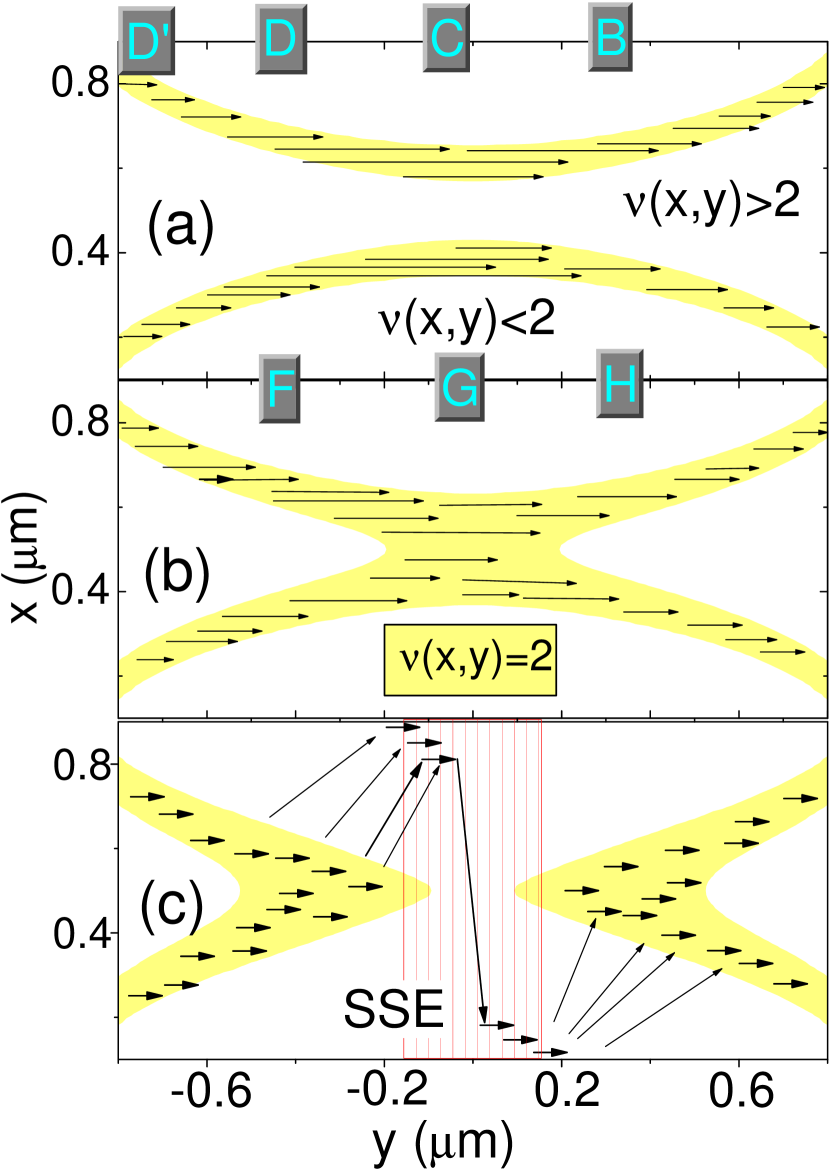
Figure 6: The calculated spatial distribution of local filling factors with integer values, $\nu(x,y)=2$ incompressible, (yellow) and compressible, (white) for three selected values of the magnetic field corresponding to a filling factor at the $y_{\perp}=0$ position $\nu=$ (a) 2.5, (b) 2.1, and (c) 1.9 at 1.6 Kelvin . The unit cell is chosen to be $1\times 2$ $\mu$m², spanning $48\times 96$ mesh points in our numerical simulation.

In Fig. 6(a), two incompressible stripes appear along the edges of the Hall bar, which are slightly curved towards the center due to the simulated bending, i.e. the external potential $V_{\rm ext}(x,y)$. The two stripes merge at the center of the Hall bar at a higher magnetic field, $\nu=2.1$, so that the center becomes completely incompressible. Whereas, at the highest magnetic field value considered here the center becomes compressible. In addition to the difference between the screening properties of the metal-like compressible (nearly perfect) and insulator-like incompressible regions (very poor), Siddiki03:125315 their transport properties are also remarkable different. As mentioned before, the compressible regions are metal-like. Therefore, scattering is finite, and hence resistance is also finite. However, at the incompressible stripes, the resistance vanishes somewhat counter intuitively since the conductance is also zero.Siddiki2004 A simple way of understanding this phenomenon is to consider the absence of backscattering within the incompressible stripes. Moreover, a simultaneous vanishing of both the longitudinal resistance and conductance is a general feature of two-dimensional systems subjected to a strong perpendicular magnetic field. Based on these arguments, the important features of the integer quantized Hall effect and local probe experiments Ahlswede02:165 can be explained.Siddiki04:condmat ; Siddiki:ijmp

The appearance of a metal-like compressible region along the current path, see Fig. 6(c) forces us to include another important ingredient in our model, namely the SSE. This phenomenon is fundamental. A fixed current imposed in a bent metal stripe in a magnetic field becomes confined to one edge of the metal due to the curvature of the system. The following two-parameter expression may be derived using the SSE theory:

$$R^{\rm SSE}=R^{\rm SSE}_{0}\frac{B}{B_{1}}\frac{e^{B/B_{1}}}{1-e^{B/B_{1}}},$$ (6)

where $R^{\rm SSE}_{0}$ is the resistance at $B_{0}$ =0, $B_{1}=r/(\mu w)$, $w$ is the Hall bar width. In Fig. 7, we provide a semi-logarithmic plot, fitting the measured longitudinal resistance $R^{L}_{\rm GH}$ of the high resistance branch with $R^{\rm SSE}$. The fit parameters $R^{\rm SSE}_{0}$=6.03 and $B_{\rm 1}$=0.015 T hold for low as well as high magnetic fields. In addition, they are very close to the corresponding values calculated by using the given mobility, the tube radius, and the width of the tube. We see, that the fitted curve follows the experimental results fairly well. In particular, at low fields, the agreement is nearly perfect since at higher filling factors the transition from compressible to incompressible (in other words metal to insulator) states at the center occurs over a very narrow magnetic field range so that the bulk remains almost always compressible. However, at higher fields the measured resistance exhibits oscillations around the theoretical curve, which are clear signatures of a compressible to incompressible transition in the bulk.

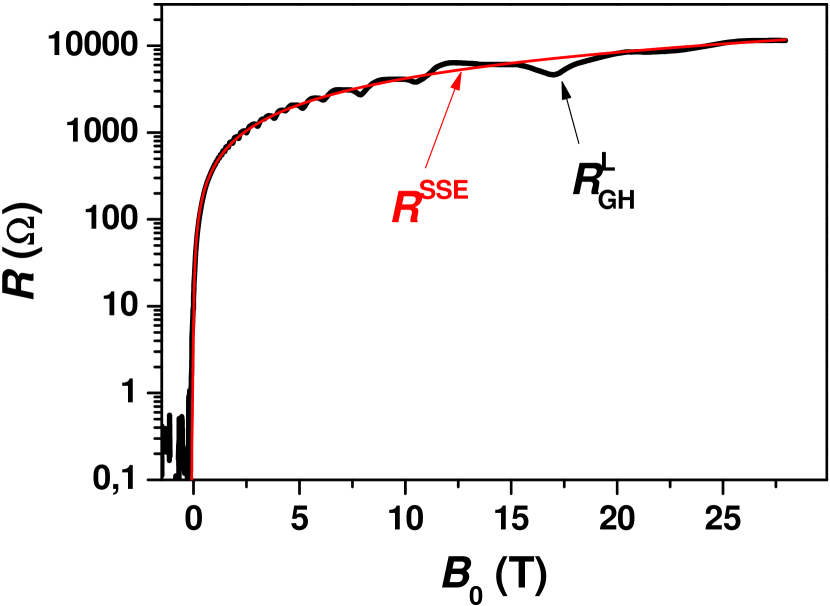
Figure 7: The measured longitudinal resistance $R^{L}_{\rm GH}$ (black thick line) vs. $B_{\rm 0}$ and the calculated theory curve $R^{\rm SSE}$ (red thin line).

Now, we can reconsider the current distribution in our model. As mentioned above the applied external current is confined to the incompressible stripes, due to the absence of backscattering. In a conventional Hall bar geometry, if an incompressible stripe percolates from source to drain contact, the system is in the quantized Hall regime, i.e. the longitudinal resistance vanishes and simultaneously the Hall resistance is quantized. Such a situation is observed in Fig. 6(a), where the longitudinal resistance measured between the leads $D-C$ (or similarly $F-G$, $C-B$, $G-H$) vanishes, while at the same time the Hall resistance is quantized, according $R^{H}_{\rm DF}=R^{H}_{\rm CG}=R^{H}_{\rm BH}=e^{2}/(2h)$. Similarly, if the center becomes incompressible, Fig. 6(b), the Hall resistance remain quantized etc. Note that now, when the higher end of the quantized Hall plateau is approached, a striking effect is observed. When the percolating incompressible stripe breaks due to the bending of the structure, the bulk becomes metal-like, and therefore the SSE comes now into play, Fig. 6(c).

First, let us discuss the Hall resistance measured between contacts $D-F$: The quantized Hall effect remains unchanged, since the bulk is well decoupled from the edges and the current is flowing from the center incompressible region. Such an argument also holds for the Hall resistance measured between the contacts $B-H$. Next, if we measure the longitudinal resistance between say $D^{\prime}-D$, we would observe that the resistance vanishes due to the existence of the percolating incompressible stripe between these two contacts. However, if we measure $R^{H}_{\rm CG}$ simultaneously, we will see that the quantization is smeared out since now the bulk behaves like an ordinary metal. At this point, due to the SSE, the current is diverted toward the edges of the Hall bar, e.g. to the upper edge on the left side of the Hall bar and to the lower edge on the right side for the one direction of the magnetic field and vice versa for the opposite field direction. Therefore, the measured longitudinal resistances $R^{L}_{\rm GH}$ and $R^{L}_{\rm DC}$ will exhibit the SSE with small deviations, resulting from the incompressible to compressible transition. This scenario implies also that the current will flow across the Hall bar at the position $y_{\perp}=0$ from one edge to the opposite one. We believe that this transition around the Hall leads $R^{H}_{\rm CG}$ also accounts for the sharp peak structure of the resistance around the transition point in $R^{L}_{\rm CB}$ and $R^{L}_{\rm FG}$, cf. Fig. 5. This effect cannot be explained by the simple Landauer Büttiker approach and indeed it would not simply occur in flat-gated samples.

In the discussion above, we have argued that the SSE becomes dominant when the center of the system is compressible and that such a transition cannot be accounted for in the 1DLS picture, where the bulk should always remain incompressible. The other features explained by the 1DLS are equally well explained by the screening theory, naturally, for the case of equilibrium. As an important point, we should emphasize that the screening theory fails to handle the non-equilibrium measurements performed by many experimental groups (for a review see Ref. Datta, ), since this theory is based on the assumption of a local equilibrium. However, in our case the filling factor gradient is NOT generated by the gates (i.e. creating non-equilibrium), but by the inhomogeneous perpendicular magnetic field. Therefore, $\delta\nu(x,y)$ is adiabatic, and the system remains in equilibrium.

V Conclusion

The quantum Hall effect for a high-mobility 2DEG on a cylinder surface show additional experimental phenomena, which indicate the presence of a specific current-density distribution in the Hall bar. The most prominent asymmetry relations hold not only for the simplified case developed for the integer filling factors, but also in a more general fashion including the transition regions between integer filling factors. Indeed, the integer filling factor case appears to be a relative rare case due to the gradual varying filling factor over the current path.

We have briefly discussed the screening theory of the integer quantum Hall effect and employed this theory to our system by simulating the filling factor gradient. The electron density is obtained self-consistently, while the (local) current distribution is derived based on a phenomenological local Ohm’s law. We have explicitly shown that due to the transition from incompressible to compressible states in the bulk, the system behaves metal-like. Therefore, SSE is observed in our measurements,

This model allows us to explain the additional sharp peaks in the resistance near the transition point, which appear in the otherwise zero-resistance edge of the Hall bar and indicate a peculiar current swing from one edge to the other. Such an effect cannot be explained by the conventional Landauer-Büttiker formalism, since in this picture the bulk remains completely insulating throughout the quantized Hall plateau regime.

- (1) V. Ya Prinz, V. A. Seleznev, A. K. Gutakovsky, A. V. Chehovskiy, V. V. Preobrazhenskii, M. A. Putyato and T. A. Gavrilova, Physica E (Amsterdam) 6, 828 (2000).
- (2) K.-J. Friedland, A. Riedel, H. Kostial, M. Höricke, R. Hey, and K.-H. Ploog, J. Electronic Mat., 90, 817 (2001).
- (3) K.-J. Friedland , R. Hey , H. Kostial, A. Riedel, and K. H. Ploog, Phys. Rev. B 045347 (2007).
- (4) A. B. Vorob’ev , K.-J. Friedland , H. Kostial, R. Hey, U. Jahn, E. Wiebicke, J. S. Yukecheva and V.Y. Prinz, Phys. Rev. B 205309 (2007).
- (5) K.-J. Friedland, R. Hey, H. Kostial, A.Riedel, phys. stat. sol. (c) 2850 (2008).
- (6) M. V. Karasev, Russian Journal of Mathematical Physics, Vol. 440 (2007).
- (7) G. Ferrari, and G. Cuoghi, Phys. Rev. Lett. , 230403 (2008).
- (8) L. A. Ponomarenko, D. T. N. de Lang, A. de Visser, V. A. Kulbachinskii, G. B. Galiev, H. Künzel, and A. M. M. Pruisken, Solid State Comm. 130, 705 (2004).
- (9) I. S. Ibrahim, V. A.Schweigert, and F. M. Peeters, Phys. Rev. B 7508 (1997).
- (10) A. V. Chaplik, JETP Lett. 72, 503 (2000).
- (11) S. Mendach, 2005 Dissertation, Fachbereich Physik, Universität Hamburg
- (12) S. Mendach, O. Schumacher, H. Welsch, Ch. Heyn, W. Hansen, and M. Holz, Appl. Phys. Lett. 88, 212113 (2006).
- (13) A. B. Vorob’ev, V. Ya. Prinz, Yu. S. Yukecheva, and A. I. Toropov, Physica E (Amsterdam) 23, 171 (2004).
- (14) S. Mendach, O. Schumacher, Ch. Heyn, S. Schnüll, H. Welsch, and W. Hansen, Physica E (Amsterdam) 23, 274 (2004).
- (15) A. Siddiki and F. Marquardt, Phys. Rev. B 75, 045325 (2007)
- (16) S. Arslan, E. Cicek, D. Eksi, S. Aktas, A. Weichselbaum and A. Siddiki, Phys. Rev. B 78, 125423 (2008)
- (17) P. M. Morse and H. Feshbach, Methods of Theoretical Physics, vol.II, p. 1240, McGraw-Hill, New York, (1953).
- (18) A. Siddiki and R. R. Gerhardts, Phys. Rev. B 68, 125315 (2003).
- (19) A. Siddiki and R. R. Gerhardts, Phys. Rev. B, 70, 195335 (2004).
- (20) E. Ahlswede, J. Weis, K. von Klitzing and K. Eberl, Physica E 12, 165 (2002).
- (21) A. Siddiki and R. R. Gerhardts, Int. J. of Mod. Phys. B, 18, 3541 (2004).
- (22) A. Siddiki and R. R. Gerhardts, Int. J. of Mod. Phys. B, 21, 1362 (2007).
- (23) S. Datta, Electronic Transport in Mesoscopic Systems, 1995, University press, Cambridge.