Dynamics of the particle - hole pair creation in graphene

Abstract

The process of coherent creation of particle - hole excitations by an electric field in graphene is quantitatively described. We calculate the evolution of current density, number of pairs and energy after switching on the electric field. In particular, it leads to a dynamical visualization of the universal finite resistivity without dissipation in pure graphene. We show that the DC conductivity of pure graphene is $\frac{\pi}{2}\frac{e^{2}}{h}$rather than the often cited value of $\frac{4}{\pi}\frac{e^{2}}{h}$. This value coincides with the AC conductivity calculated and measured recently at optical frequencies. The effect of temperature and random chemical potential (charge puddles) are considered and explain the recent experiment on suspended graphene. A possibility of Bloch oscillations is discussed within the tight binding model.

1. Introduction. It has been demonstrated recently that a graphene sheet, especially one suspended on leads, is one of the purest electronic systems. Electronic mobility reaches values of $2\cdot 10^{5}cm^{2}/\left(Vs\right)$ and might be yet improved GeimPRL08 ; Andrei08 indicating that transport in samples of submicron length is most likely ballistic. In a simplified model of a single graphene sheet (neglecting scattering processes and electron interactions) the chemical potential is located right between the valence and conductance bands and the Fermi ”surface” consists of two Dirac points of the Brillouin zone Castro . A lot of effort has been devoted to the question of transport in pure graphene due to the surprising fact that the DC conductivity is finite without any dissipation process present. A widely accepted value of the ”minimal conductivity” at zero temperature,

$$\sigma_{1}=\frac{4}{\pi}\frac{e^{2}}{h},$$ (1)

was calculated very early on using the Kubo formula in a simplified Dirac model as well as in the tight binding model Fradkin ; Ando02 ; Castro ; Katsnelson06 . Within this approach one starts with the AC conductivity and takes a zero frequency limit typically with certain ”regularizations” (like finite temperature, disorder strength $\eta$ etc.) made and removed at the end of the calculation. As noted by Ziegler Ziegler06 the order of limits makes a difference and several other values different from $\sigma_{1}$ were provided for the same system. The standard value $\sigma_{1}$ is obtained using a rather unorthodox procedure when the DC limit $\omega\rightarrow 0$ is made before the zero disorder strength limit $\eta\rightarrow 0$ is taken. If the order of limits is reversed one obtains Ziegler06

$$\sigma_{2}=\frac{\pi}{2}\frac{e^{2}}{h}.$$ (2)

When the limit is taken holding $\omega=\eta$ one can even obtain a value of $\sigma_{3}=\pi\frac{e^{2}}{h}$ Ziegler06 , thus solving the ”missing $\pi$” problem. Indeed, at least early experiments on graphene sheets on Si substrates provided values roughly 3 times larger than $\sigma_{1}$ Novoselov05 . Recent experiments on suspended graphene Andrei08 demonstrated that the DC conductivity is lower, $1.7\sigma_{1}$, as temperature is reduced to $4K$. Hence one still faces the question of what is the proper theoretical value. Since the conductivity of clean graphene in the infinite sample is a well defined physical quantity there cannot be any ambiguity as to its value.

In contrast both the experimental and the theoretical situation for the AC conductivity in the high frequency limit is quite different. The theoretically predicted value in the Dirac model is $\sigma_{2}$ independent of frequency under condition $\omega>>T/\hbar$ Ando02 ; Varlamov07 . The Dirac model becomes inapplicable when $\omega\$is of order of $\gamma/\hbar=4\cdot 10^{15}Hz$ or larger, where $\gamma=2.7eV$ is the hopping energy of graphene. It was shown theoretically using the tight binding model and experimentally in GeimScience08 that the optical conductivity at frequencies higher or of order $\gamma/\hbar$ becomes slightly larger than $\sigma_{2}$. Moreover, in light transmittance measurements at frequencies down to $2.5\cdot 10^{15}Hz$ it was found equal to $\sigma_{2}$ within 4%. The model does not contain any other time scale capable of changing the limiting value of AC conductivity all the way to $\omega->0$. Therefore one would expect that the DC conductivity even at zero temperature is $\sigma_{2}$ rather than $\sigma_{1}$. As we show in this note this is indeed the case.

The basic physical effect of the electric field is a coherent creation of electron - hole pairs mostly near Dirac points. To effectively describe this process we develop a dynamical approach to charge transport in clean graphene using the ”first quantized” approach to pair creation physics similar to that used in relativistic physics Gitman . To better visualize the phenomenon of resistivity without dissipation, we describe an experimental situation as closely as possible by calculating directly the time evolution of the electric current after switching on an electric field. In this way the use of a rather formal Kubo or Landauer formalism is avoided and as a result no regularizations are needed. The effects of temperature and of charge fluctuations or ”puddles” are investigated and explain the temperature dependence of conductivity measured recently in suspended graphene Andrei08 . Although we consider an infinite sample the dynamical approach allows us to obtain qualitative results for finite samples by introducing time cutoffs like ballistic flight time. Various other factors determining transport can be conveniently characterized by time scales like the relaxation time for scattering of phonons or impurities.

2. Time evolution of the current density at zero temperature. Electrons in graphene are described sufficiently well by the 2D tight binding model of nearest neighbour interactions Castro , namely with (second quantized) Hamiltonian being sum over all the links connecting sites on two triangular sublattices $A,B$. The Hamiltonian in momentum space is

$$\widehat{H}=\int_{BZ}\begin{pmatrix}c_{A}^{{\dagger}}&c_{B}^{{\dagger}}\end{pmatrix}H\begin{pmatrix}c_{A}\\ c_{B}\end{pmatrix};\text{ \ \ }H=\begin{pmatrix}0&h\\ h^{\ast}&0\end{pmatrix},$$ (3)

where $h\left(k\right)=-\gamma\sum_{\alpha}e^{i\mathbf{k}\cdot\delta_{\alpha}}$ with $\gamma$ being the hopping energy; $\delta_{1}=\frac{a}{3}\left(0,\sqrt{3}\right),$ $\ \delta_{2,3}=\frac{a}{3}\left(\pm\frac{3}{2},-\frac{\sqrt{3}}{2}\right)$ are the locations of nearest neighbours on the honeycomb lattice separated by distance $a\simeq 3\mathring{A}$. In the Brillouin zone of the lattice there are two Dirac points $K_{-}=\frac{2\pi}{a}\left(\frac{1}{3},\frac{1}{\sqrt{3}}\right),\ K_{+}=\frac{2\pi}{a}\left(\frac{2}{3},0\right)$ in which the energy gap between the valence and the conduction band vanishes. Expansion around $K_{-}$, $h\left(k\right)=\hslash v_{g}\exp\left(-i\frac{\pi}{3}\right)\left(\Delta k_{x}+i\Delta k_{y}\right),$ where the graphene velocity is $v_{g}=\frac{\sqrt{3}}{2}\frac{a\gamma}{\hslash},$ leads to relativistic equations for the Weyl field constructed as $\psi_{1}=\psi_{1}^{W},$ $\ \psi_{2}=e^{-i\frac{\pi}{3}}\psi_{2}^{W}$.

Let us first consider the system in a constant and homogeneous electric field along the $y$ direction switched on at $t=0.$ It is described by the minimal substitution $\mathbf{p}=\hslash\mathbf{k}+\frac{e}{c}\mathbf{A}$ with vector potential (choosing a gauge in which the scalar potential is zero) $\mathbf{A}=\left(0,-cEt\right)$. Since the crucial physical effect of the field is a coherent creation of electron - hole pairs mostly near Dirac points a convenient formalism to describe the pair creation is the ”first quantized” formulation described in detail in Gitman . The second quantized state at $T=0$ which evolves from the zero field state in which all the negative energy ($-\left|h\left(k\right)\right|$) states are occupied is uniquely characterized by the first quantized amplitude $\psi_{k}\left(t\right)=\begin{pmatrix}\psi_{k1}\left(t\right)\\ \psi_{k2}\left(t\right)\end{pmatrix}$ obeying the matrix Schroedinger equation $i\hslash\partial_{t}\psi=H\psi$ in sublattice space with the initial condition

$$\psi_{k}\left(t=0\right)=u_{k};\text{ \ }u_{k}=\frac{1}{\sqrt{2}}\begin{pmatrix}1\\ -h^{\ast}/\left|h\right|\end{pmatrix}.$$ (4)

Here $u_{k}$ is found as a negative energy solution of the time independent Schroedinger equation prior to switching on the electric field, $Hu_{k}=-\left|h\right|u_{k}$.

A physical quantity is usually conveniently written in terms of $\psi$. For example the current density (multiplied by factor $2$ due to spin) is

$$J_{y}=-2e\int_{BZ}\psi_{k}^{{\dagger}}\left(t\right)\frac{\partial H\left(\mathbf{p}\right)}{\partial p_{y}}\psi_{k}\left(t\right)$$ (5)

To first order in electric field $\psi_{k}=e^{\frac{i}{\hslash}\left|h\right|t}\left(u_{k}+E\xi_{k}+...\right)$ and consequently $J_{y}=J_{0}+E\sigma,$ where

$$J_{0} = -\frac{2e}{\hslash}\int_{BZ}u_{k}^{{\dagger}}\frac{\partial H\left(\mathbf{k}\right)}{\partial k_{y}}u_{k}=\frac{2e}{\hslash}\int_{BZ}\frac{\partial\left|h\right|}{\partial k_{y}};$$ (6)

$$\sigma\left(t\right) = \int_{BZ}\sigma_{k}\left(t\right);$$

$$\sigma_{k}\left(t\right) = -\frac{2e}{\hslash}\left[u_{k}^{{\dagger}}\frac{\partial H\left(\mathbf{k}\right)}{\partial k_{y}}\xi_{k}+\xi_{k}^{{\dagger}}\frac{\partial H\left(\mathbf{k}\right)}{\partial k_{y}}u_{k}-\frac{e}{\hslash}tu_{k}^{{\dagger}}\frac{\partial^{2}H\left(\mathbf{k}\right)}{\partial k_{y}^{2}}u_{k}\right].$$

The solution of the Schroedinger equation for the correction $\xi_{k}$ is

$$\xi_{k} = \frac{ie}{2\hslash^{2}}t^{2}\frac{\partial\left|h\right|}{\partial k_{y}}u_{k}$$

$$+\frac{ie}{8\left|h\right|^{3}}\left(h^{\ast}\frac{\partial h}{\partial k_{y}}-cc\right)\left(1-e^{-2i\left|h\right|t/\hslash}-\frac{2i\left|h\right|}{\hslash}t\right)v_{k},$$

where $v_{k}=\frac{1}{\sqrt{2}}\begin{pmatrix}1\\ h^{\ast}/\left|h\right|\end{pmatrix}$. Substituting this into Eq.(6) the conductivity becomes

$$\sigma_{k}\left(t\right)=\frac{e^{2}}{\hslash}\left[-\frac{\partial^{2}\left|h\right|}{\partial k_{y}^{2}}\frac{2t}{\hslash}-\frac{1}{4\left|h\right|^{4}}\left(h^{\ast}\frac{\partial h}{\partial k_{y}}-cc\right)^{2}\sin\left(\frac{2\left|h\right|}{\hslash}t\right)\right].$$ (8)

The zero field current $J_{0}$ and the first term (linear in time) in the conductivity vanish upon integration over the Brillouin zone, since one can choose it to be $\int_{BZ}=\int_{-\pi/a}^{\pi/a}dk_{x}\int_{-2\pi/\left(3^{1/2}a\right)}^{2\pi/\left(3^{1/2}a\right)}dk_{y}$ and the integrand is a derivative of a periodic function.

The integral of the second part (oscillatory in time) of $\sigma_{k}\left(t\right)$ gives the result shown in Fig.1. After an initial increase over the natural time scale $t_{\gamma}\equiv\hslash/\gamma=2.5\cdot 10^{-16}s$, it approaches $\sigma_{2}$, Eq.(2), via oscillations. The amplitude of oscillations decays as a power

$$\frac{\sigma}{\sigma_{2}}=1+\frac{\sin\left(2t/t_{\gamma}\right)}{2t/t_{\gamma}}$$ (9)

for $t>>t_{\gamma}$. The limiting value is dominated by contributions from the vicinity of the two Dirac points in the integral of Eq.(6). The contribution of a Dirac point is obtained for $t>>t_{\gamma}$ by integrating to infinity (in polar coordinates centered at the Dirac point)

$$\frac{\sigma}{2}=\frac{e^{2}}{\hslash}\frac{1}{\left(2\pi\right)^{2}}\int_{\varphi=0}^{2\pi}\int_{q=0}^{\infty}\sin\left(\varphi\right)^{2}\frac{\sin\left(2v_{g}qt\right)}{q}=\frac{e^{2}}{h}\frac{\pi}{4},$$ (10)

does not influence the result.

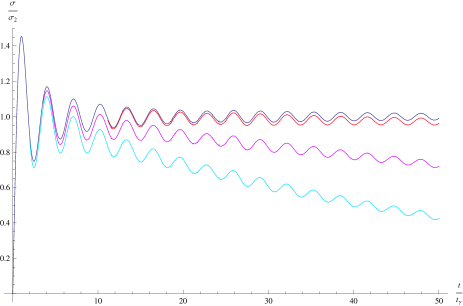
Figure 1: Evolution of the current density $\sigma\left(t\right)=J\left(t\right)/E$ after a DC electric field is switched on at $t=0$. Unit of time is $t_{\gamma}=\hbar/\gamma$. Conductivity is compared to its ”dynamical” value $\sigma_{2}=\frac{\pi}{2}\frac{e^{2}}{h}$. The zero temperature conductivity (blue) approaches $\sigma_{2}$, while finite temperature depresses the pair creation and eventually the current density vanishes as $\frac{1}{tT}$.

A physical picture of this resistivity without dissipation is as follows. The electric field creates electron - hole excitations in the vicinity of the Dirac points in which excitations are massless relativistic fermions. For such particles the absolute value of the velocity is $v_{g}$ and cannot be altered by the electric field and is not related to the wave vector $\mathbf{k}$. On the other hand, the orientation of the velocity is influenced by the applied field. The electric current is $e\mathbf{v}$, thus depending on orientation, so that its projection on the field direction $y$ is increased by the field. The energy of the system (calculated in a way similar to the current) is increasing continuously if no channel for dissipation is included. Obviously at some time the system goes beyond linear response into Bloch oscillations which are briefly discussed below. We have performed a similar calculation for the evolution of the current density for an AC electric field switched on at $t=0$. After a short transient one obtains the value of the DC conductivity $\sigma_{2}$ independent of frequency. This is consistent with both the Kubo formula derivations Varlamov07 and optical experiments GeimScience08 .

3. The temperature dependence and effect of charge ”puddles”. At finite temperature $T$ within the first quantized formalism one adds the contributions of all the energies including positive ones weighted with the Boltzmann factor. Due to electron - hole symmetry the contribution to conductivity of a positive energy state with momentum $\mathbf{k}$ is minus that of the contribution of the negative energy state with the same wave vector. This results in the thermal factor

$$\sigma_{T}\left(t\right)=\int_{BZ}\tanh\left(\frac{\left|h\right|}{T}\right)\sigma_{k}\left(t\right).$$ (11)

The first term still vanishes, while the second gives a depressed value compared to that at $T=0$, see Fig. 1. Moreover, the conductivity vanishes at the large time limit. This is easy to appreciate qualitatively: the contributions from the vicinity of the Dirac points, $\left|h\right|<<T$, which were the main contributors to $\sigma\left(T\right)$ are effectively suppressed. Physically this suppression can be understood as follows. As mentioned above the finite resistivity of pure graphene is due to pair creation by an electric field near Dirac points. The pair creation is maximal when in the initial state the valence band is full and the conductance band is empty. Thermal fluctuations create pairs as well. In the formalism we adopted the finite temperature initial state is described by the density matrix which specified the number of incoherent pairs present in the energy range near the Dirac points. Therefore pair creation by an electric field is less intensive due to the diminished phase space available and the conductivity vanishes at large times.

Under assumption of Dirac point dominance, $T<<\gamma$ (definitely covering the temperature range $T<200K$ beyond which scattering is not negligible GeimPRL08 ), the expression can be simplified in the same way as Eq.(10),

$$\sigma_{T}\left(t\right)=\frac{e^{2}}{h}\int_{q=0}^{\infty}\tanh\left(\frac{\hbar v_{g}q}{T}\right)\frac{\sin\left(2v_{g}tq\right)}{q}\text{,}$$ (12)

and is a monotonically decreasing function of the product $tT$. For $t>>t_{\gamma,}$ $\sigma_{T}\left(t\right)=\frac{e^{2}}{h}\frac{\hbar}{tT}$.

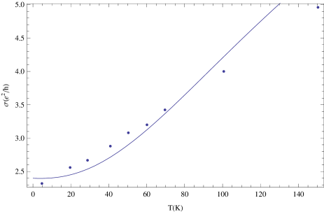
Figure 2: The minimal conductivity as a function of temperature for time $t_{bal}=500t_{\gamma}$ is compared with measured in the $0.5\mu m$ long sample in ref.Andrei08 . Values for the random Fermi energy are also taken from ref.Andrei08 .

Assuming ballistic transport in a finite sample of submicron length determining an effective ballistic time $t_{b}\,$, this contribution cannot explain the increase of conductivity with temperature in suspended graphene reported in Andrei08 . However, there is an important source of positive contribution to conductivity even in the ballistic regime. It was clearly demonstrated that a sample close to minimal conductivity consists of positively and negatively charged puddles. This means effectively that even at minimal conductivity the chemical potential $\mu$ locally is finite, rather than zero, albeit small on average. Physically this implies that in addition to the novel constant contribution due to pair creation, there is an ordinary contribution due to acceleration of electrons like in ordinary metal. In ballistic regime it grows linearly with time.

The experiment Andrei08 shows that the amplitude of the random Fermi energy increases linearly with temperature $\mu_{T}=\mu_{0}+\alpha T$. For example, for the $0.5\mu m$ long sample $\mu_{0}=8meV$ and $\alpha=0.1meV/K$. The difference between $\sigma_{\mu}$ and $\sigma_{\mu=0}$ is equal to the integral in Eq.(6) over the two regions around the Dirac points determined by $\left|h\left(\mathbf{k}\right)\right|<\mu$. That way one obtains for $t>>t_{\gamma}$

$$\sigma_{\mu}\left(t\right)-\sigma_{\mu=0}\left(t\right)=\frac{e^{2}}{h}\left[\frac{\sqrt{3}\mu t}{\hslash}-Si\left(\frac{\sqrt{3}\mu t}{\hslash}\right)\right],$$ (13)

which is a monotonically increasing function of the product $\mu t$ only ($Si$ is the sine integral function). In Fig.2 we fit the value of the ballistic effective time $t_{bal}$ $\simeq 2\cdot 10^{-13}s$, which is of the same order of magnitude as for the $0.5\mu m$ long sample, $L/v_{g}\simeq 5\cdot 10^{-13}s$.

4. Discussion and summary.

To summarize, we studied the dynamics of the particle - hole pair creation by calculating the time evolution of current density, particle - hole number and energy after the electric field is switched on. After a brief transient period (of order of several $t_{\gamma}=\hslash/\gamma$) the current density approaches a finite value. The minimal DC electric conductivity at zero temperature is $\frac{\pi}{2}\frac{e^{2}}{h}$, different from an accepted value $\frac{4}{\pi}\frac{e^{2}}{h}$. The later value was obtained for nonideal systems by taking various limits (impurity strength etc.) or in theory of finite size effects Beenaker and does not characterize an ideal pure infinite graphene sheet. At finite temperature $T$ the current density diminishes on the scale of $t_{T}=\hslash/T=\frac{\gamma}{T}t_{\gamma}$. Therefore the phenomenon of finite resistivity without dissipation disappears unless there exists a shorter time scale intercepting the process like $2\pi/\omega$ for AC field, relaxation time $\tau$ for scattering off impurities or phonons or ballistic flight time $t_{bal}$ for finite samples. The effect of small random chemical potential was also considered.

Let us now address the issue of the validity of the linear response approximation used. Since the model does not provide a channel of dissipation, the problem is nontrivial. Where does the Joule heat $\sigma E^{2}$ go? The dynamical approach allows us to calculate the evolution of energy as well as to go beyond linear response. Of course the energy continuously increases with time and at certain time approaches the conduction band edge at which stage linear response breaks down. We calculated the evolution of current density, energy and pair number beyond linear response and found that Bloch oscillations set in with a period of $t_{Bloch}=\frac{\hslash}{eaE}=\frac{\gamma}{eaE}t_{\gamma}$. The range of applicability of the linear response was also determined. The average current over larger times is zero. This means that at very high fields the minimal conductivity phenomenon disappears. However in order to reach the conditions for observation of the Bloch oscillations in graphene all other time scales $\tau,t_{T},t_{bal},2\pi/\omega$ should be larger than $t_{Bloch}$. Additional phenomena beyond linear response as well as their relation to the Schwinger’s calculation of the pair creation rate [ Schwinger ; Gitman ] is under investigation.

- (1) S.V. Morozov et al, Phys. Rev. Lett, 100, 016602 (2008).
- (2) X. Du, I. Skachko, A. Barker and E. Y. Andrei, Nature Nanotechnology 3, 491 (2008).
- (3) R.R. Nair et al, Science 320, 1308 (2008).
- (4) A. H. Castro Neto et al, Rev. Mod. Phys. to be published (2008), arXiv:0709.1163; V. P. Gusynin, S. G. Sharapov and J. P. Carbotte, Int. J. Mod. Phys. B 21, 4611 (2007).
- (5) E. Fradkin, Phys. Rev. B 33, 3257 (1986); P.A. Lee, Phys. Rev. Lett, 71, 1887 (1993); A.W.W. Ludwig et al, Phys. Rev. B 50, 7526, (1994); V. P. Gusynin and S. G. Sharapov, Phys. Rev. B 73, 245411 (2006); N.M.R. Peres et al, Phys. Rev. B73, 125411 (2006).
- (6) T. Ando, Y. Cheng and H. Suzuura, J. Phys. Soc. Jap. 71, 1318 (2002).
- (7) K. Ziegler, Phys. Rev. Lett. 97, 266802 (2006); Phys. Rev. B75, 233407 (2007).
- (8) K.S. Novoselov et al, Nature 438, 197 (2005); Y. Zhang et al, Nature 438, 201 (2005).
- (9) M.I. Katsnelson, Eur. Phys. J. B 51, 157 (2006).
- (10) L.A. Falkovsky and A.A. Varlamov, Eur. Phys. J. B 56, 281 (2007).
- (11) T. Stauber, N.M.R. Peres and A. H. Castro Neto, Phys. Rev. B78, 085418, (2008).
- (12) E.S. Fradkin, D.M. Gitman and S.M. Shvartsman, Quantum Electrodynamics with Unstable Vacuum (Springer-Verlag, Berlin 1991).
- (13) J. Tworzydlo et al, Phys. Rev. Lett. 96, 246802 (2006).
- (14) J. Schwinger, Phys. Rev. 82, 664 (1951); G. Dunne and T. Hall, Phys. Rev. D58, 105022 (1998); S.P. Kim, H.K. Lee and Y. Yoon, Phys. Rev. D78, 105013 (2008).