Hidden Symmetries and Black Holes

Abstract

The paper contains a brief review of recent results on hidden symmetries in higher dimensional black hole spacetimes. We show how the existence of a principal CKY tensor (that is a closed conformal Killing-Yano 2-form) allows one to generate a ‘tower’ of Killing-Yano and Killing tensors responsible for hidden symmetries. These symmetries imply complete integrability of geodesic equations and the complete separation of variables in the Hamilton-Jacobi, Klein-Gordon, Dirac and gravitational perturbation equations in the general Kerr-NUT-(A)dS metrics. Equations of the parallel transport of frames along geodesics in these spacetimes are also integrable.

1 Introduction

There are several reasons why a subject of higher dimensional black holes becomes so popular recently. The idea that the spacetime can have more than four dimensions is very old. Kaluza and Klein used this idea about 80 years ago in their attempts to unify electromagnetism with gravity. The modern superstring theory is consistent (free of conformal anomalies) only if the spacetime has a fixed number (10) of dimensions. Usually it is assumed that extra dimensions are compactified. The natural size of compactification in the string theory is of order of the Planckian scale. In recently proposed models with large extra-dimensions it is also assumed that the spacetime has more than 3 spatial dimensions. A new feature is that the size of the extra dimensions can be much larger than the Planckian size, $10^{-33}$cm (up to 0.1mm) . In order to escape contradictions with observations it is usually assumed that the matter and fields (except the gravitational one) are confined to a four-dimensional brane representing our world, while the gravity can propagate in the bulk. In so called ADD models [1, 2] the extra dimensions are flat. In the Randall-Sundrum models [3, 4] the bulk 5D spacetime is curved and it has anti-deSitter asymptotics. Black holes in the string theory and in the models with larger extra dimensions play an important role serving as probes of extra dimension. Study of higher dimensional black holes is a very important problem of the modern theoretical and mathematical physics.

One of the main features of the models with large extra dimensions is a prediction that gravity becomes strong at small distances. This conclusion implies that for the particle collision with the energy of the order of TeV the gravitational channel would be as important as the electroweak channel of the interaction. Under these conditions two qualitatively new effects are possible: (1) bulk emission of gravitons, and (2) mini-black-hole production. These effects have been widely discussed in the connection with the expected new data at the Large Hadronic Collider (LHC) (see e.g. [5] and references therein). Hawking radiation produced by such mini black holes has several observable features which allows one, in principle, to single out such events in observations [6, 7, 8].

When the gravitational radius of a black hole is much smaller than the size of extra dimensions and the tension of the brane is neglected one can consider a the black hole as an isolated one. Such a black hole is described by a solution of the higher dimensional Einstein equations which is asymptotically flat or has (A)dS asymptotics. It was shown that besides ‘standard’ black holes with a spherical topology of the horizon, in higher dimensions there exist black objects with a different horizon topology. Black rings [9] and black saturns [10] are examples of such solutions in the 5D spacetime. For a review of higher dimensional black objects and their properties see, e.g., [11].

The most general known higher dimensional black hole solution of the Einstein equations with the spherical topology of the horizon is a Kerr-NUT-(A)dS metric which was discovered recently [12]. The metric belongs to the special algebraic type D [13] of the higher-dimensional algebraic classification [14, 15, 16]. This makes these metrics quite different from the black ring and black saturn type solutions, which are of type $I_{i}$ [16]. In this paper we review properties of the higher dimensional black hole solutions and, especially, their hidden symmetries. We demonstrate that the properties of the higher dimensional black holes, in many aspects are similar to the properties of the four dimensional black holes.

An isolated stationary black hole in 4-dimensional asymptotically flat spacetime is uniquely specified by two parameters, its mass and angular momentum. The corresponding Kerr metric possesses a number of properties, which was called by Chandrasekhar ‘miraculous’. In particular the Kerr metric allows the separation of variables in the geodesic Hamilton-Jacobi equation and a massless field equations. These properties look ‘miraculous’ since the spacetime symmetries of the Kerr metric are not sufficient to explain them. Really, spacetime symmetries are ‘responsible’ for two integrals of motion, the energy and the azimuthal component of the angular momentum. This, together with the conservation of ${\mbox{\boldmath$p$}}^{2}$, gives only 3 integrals of motion. Carter [17, 18] constructed the fourth required integral of motion, which is quadratic in momentum and is connected with the Killing tensor [19]. Penrose and Floyd [20] showed that this Killing tensor is a ‘square’ of an antisymmetric Killing-Yano tensor [21].

In many aspects a Killing-Yano tensor is more fundamental than a Killing tensor. Namely, its ‘square’ is always Killing tensor, but the opposite is not generally true (see, e.g., [22]). It was shown by Collinson [23] a $4$–dimensional vacuum spacetime which admits a non–degenerate Killing-Yano tensor is of the type $\bf D$. All the vacuum type $\bf D$ solutions were obtained by Kinnersley [24]. Demianski and Francaviglia [25] showed that in the absence of the acceleration these solutions admit Killing and Killing-Yano tensors. It should be also mentioned that if a spacetime admits a non–degenerate Killing-Yano tensor it always has at least one Killing vector [26].

Separability of massless and massive field equations (including the gravitational perturbations) in the 4D Kerr metric [27, 28, 29, 30, 31] is a direct consequence of the hidden symmetries. The separability property plays a key role in study of properties of rotating black holes, including the proof of their stability and the calculation of Hawking radiation.

In 2003 is was discovered that five-dimensional Myers-Perry black holes possess a Killing tensor [32, 33]. This makes geodesic equations completely integrable (see e.g [34] where the cross-section of particles and photons for 5D black holes was studied.) After this a lot of attempts were made to study the hidden symmetries of the higher dimensional black holes. In the most of these publications an additional assumption was made. Namely special conditions were imposed on the rotation parameters of a black hole which enhance the symmetry of these solutions. In 2007 it was discovered that Myers-Perry metrics with arbitrary rotation parameters, as well as a general Kerr-NUT-(A)dS metrics possesses a closed conformal Killing-Yano 2-form [35, 36]. This result was used to demonstrate that the general high dimensional black hole solutions in many aspects are similar to their four dimensional ‘cousin’. This paper contains a brief review of the recent development of the theory of higher dimensional black holes and hidden symmetries (see also [37, 38, 39]).

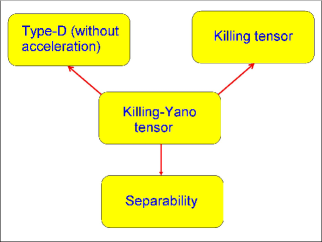
Figure 1: Killing-Yano tensors in 4D spacetime and their properties.

2 Hidden symmetries

The concept of symmetries is one of the most powerful tools of modern theoretical physics. Noether’s theorem relates continuous symmetries to conservation laws. The most fundamental of them are connected with the symmetries of the background spacetime. A curved spacetime possesses a symmetry if there exists a diffeomorphism preserving the geometry. Consider a one-parameter family of continuous transformations

$$x^{a}\to\bar{x}^{a}=F^{a}(x,t)\,.$$ (1)

Denote by $\xi$ a vector field generating these transformations

$$\xi^{a}=\left.{dF^{a}\over dt}\right|_{t=0}\,.$$ (2)

Invariance of the metric $g$ under the transformations Eq.(1) implies that

$${\cal L}_{{\mbox{\boldmath$\xi$}}}g_{ab}=0\,,$$ (3)

where ${\cal L}_{{\mbox{\boldmath$\xi$}}}$ is the Lie derivative. A generator $\xi$ of the continuous symmetry transformation (isometry) is called a Killing vector. The equation Eq.(3) can be identically rewritten in the form

$$\xi_{(a;b)}=0\,.$$ (4)

In the presence of the symmetry generated by the Killing vector $\xi$ geodesic equations possess an integral of motion

$$P_{\xi}=\xi_{a}u^{a}\,,$$ (5)

where $u^{a}=dx^{a}/d\lambda$ is a tangent vector to a geodesic and $\lambda$ is an affine parameter. Really,

$${dP_{\xi}\over d\lambda}=u^{b}u^{a}\xi_{a;b}+u^{b}u^{a}_{\ ;b}\xi_{a}=0\,.$$ (6)

The first term in the right hand side vanishes because of the Killing equation Eq.(4), while the second one vanishes because of the geodesic equation of motion $u^{b}u^{a}_{\ ;b}=0$.

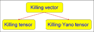
Figure 2: Possible generalizations of the Killing vector.

A Killing tensor $K_{a_{1}\ldots a_{k}}$ is a natural symmetric generalization of the Killing vector. Let us assume that for any geodesic with a tangent vector $u^{a}$ the following object

$$P_{K}=K_{a_{1}\ldots a_{k}}u^{a_{1}}\ldots u^{a_{k}}\,$$ (7)

is concerved

$${dP_{K}\over d\lambda}=0\,.$$ (8)

For a geodesic motion

$${dP_{K}\over d\lambda}\equiv u^{b}u^{a_{1}}\ldots u^{a_{k}}K_{a_{1}\ldots a_{k};b}$$ (9)

Since this relation is valid for an arbitrary $u$ one has

$$K_{(a_{1}\ldots a_{k};b)}=0\,.$$ (10)

A symmetric tensor $K_{(a_{1}\ldots a_{k})}$ obeying the relation Eq.(10) is called a Killing tensor.

A Killing-Yano tensor $f_{a_{1}\ldots a_{k}}$ is an antisymmetric generalization of the Killing vector. Let us assume that for any geodesic with a tangent vector $u^{a}$ the following object

$$P_{a_{1}\ldots a_{k-1}}=f_{a_{1}\ldots a_{k}}u^{a_{k}}\,$$ (11)

is parallel propagated along the geodesic

$$u^{b}P_{a_{1}\ldots a_{k-1};b}=0\,.$$ (12)

Using the geodesic equation one obtains

$$f_{a_{1}\ldots a_{k};b}u^{a_{k}}u^{b}=0\,.$$ (13)

Since this relation is valid for an arbitrary $u^{a}$ it implies

$$f_{a_{1}\ldots(a_{k};b)}=0\,.$$ (14)

A skewsymmetric tensor $f_{a_{1}\ldots a_{k}}$ obeying this relation is called a Killing-Yano tensor.

It is easy to show that if $f_{a_{1}\ldots a_{k}}$ is a Killing-Yano tensor then

$$K_{ab}=f_{aa_{1}\ldots a_{k-1}}f^{\ \ a_{1}\ldots a_{k-1}}_{b}$$ (15)

is a Killing tensor.

An important generalization of the symmetry Eq.(3) is a conformal symmetry. A conformal Killing vector $\xi$ generating such a transformation obeys the equation

$${\cal L}_{{\mbox{\boldmath$\xi$}}}g_{ab}=\beta(x)g_{ab}\,,$$ (16)

or, equivalently

$$\xi_{(a;b)}=\tilde{\xi}g_{ab}\,,\hskip 14.22636pt\tilde{\xi}=D^{-1}\xi^{b}_{\ \ ;b}\,.$$ (17)

The corresponding expression Eq.(5) is conserved for null geodesics. The conformal generalizations of the Killing and Killing-Yano tensors are defined as follows. A symmetric tensor $K_{a_{1}a_{2}\ldots a_{p}}=K_{(a_{1}a_{2}\ldots a_{p})}$ is called a conformal Killing tensor if it obeys the equation

$$K_{(a_{1}a_{2}\ldots a_{p};b)}=g_{b(a_{1}}\tilde{K}_{a_{2}\ldots a_{p})}\,.$$ (18)

It is easy to show that a symmetrized tensor product of two conformal Killing tensors is again a conformal Killing tensor. Similarly, a tensor product of two Killing tensors is again a Killing tensor. A (conformal) Killing tensor is called reducible if it can be written as a linear combination of tensor products of lower rank (conformal) Killing tensor. If a Killing tensor of rank $q$ is reducible, the corresponding conserved quantity for a geodesic motion, which is a polynomial of rank $q$ in momentum, can be written as a linear combination of products of conserved quantities of lower than $q$ powers in momentum. It means that a reducible Killing tensor does not generate any new independent conserved quantities.

An antisymmetric generalization of the conformal Killing vector is known as a conformal Killing-Yano tensor. An antisymmetric tensor $h_{a_{1}a_{2}\ldots a_{p}}=h_{[a_{1}a_{2}\ldots a_{p}]}$ is called a conformal Killing-Yano tensor (or, briefly, CKY tensor) if it obeys the following equation [40]

$$\nabla_{(a_{1}}h_{a_{2})a_{3}\ldots a_{p+1}}=g_{a_{1}a_{2}}\tilde{h}_{a_{3}\ldots a_{p+1}}-(p-1)g_{[a_{3}(a_{1}}\tilde{h}_{a_{2})\ldots a_{p+1}]}\,.$$ (19)

By tracing the both sides of this equation one obtains the following expression for $\tilde{{\mbox{\boldmath$h$}}}$

$$\tilde{h}_{a_{2}a_{3}\ldots a_{p}}={1\over D-p+1}\nabla^{a_{1}}h_{a_{1}a_{2}\ldots a_{p}}\,.$$ (20)

3 Conformal Killing-Yano tensors

Let us discuss properties of the conformal Killing-Yano (CKY) tensors in more details. The CKY tensors are forms and operations with them are greatly simplified if one uses the ”language” of differential forms. We just remind some of the relations we use in the present paper. If ${\mbox{\boldmath$\alpha$}}_{p}$ and ${\mbox{\boldmath$\beta$}}_{q}$ are $p$- and $q$-forms, respectively, the external derivative ($d$) of their external product ($\wedge$) obeys a relation

$$d({\mbox{\boldmath$\alpha$}}_{p}\wedge{\mbox{\boldmath$\beta$}}_{q})=d{\mbox{\boldmath$\alpha$}}_{p}\wedge{\mbox{\boldmath$\beta$}}_{q}+(-1)^{p}{\mbox{\boldmath$\alpha$}}_{p}\wedge d{\mbox{\boldmath$\beta$}}_{q}\,.$$ (21)

A Hodge dual $*{\mbox{\boldmath$\alpha$}}_{p}$ of the $p$-form ${\mbox{\boldmath$\alpha$}}_{p}$ is $(D-p)$-form defined as

$$*{\mbox{\boldmath$\alpha$}}_{p}\Leftrightarrow(*\alpha)_{a_{1}\ldots a_{D-p}}={1\over p!}\alpha^{b_{1}\ldots b_{p}}e_{b_{1}\ldots b_{p}a_{1}\ldots a_{D-p}}\,,$$ (22)

where $e_{a_{1}\ldots a_{D}}$ is a totally anti-symmetric tensor. The exterior co-derivative $\delta$ is defined as follows

$$\delta{\mbox{\boldmath$\alpha$}}_{p}=(-1)^{p}\epsilon_{p}*d*{\mbox{\boldmath$\alpha$}}_{p}\,,\hskip 5.69046pt\epsilon_{p}=(-1)^{p(D-p)}{\mbox{det}(g)\over|\mbox{det}(g)|}\,.$$ (23)

One also has $**{\mbox{\boldmath$\alpha$}}_{p}=\epsilon_{p}{\mbox{\boldmath$\alpha$}}_{p}$.

If $\{{\mbox{\boldmath$e$}}_{a}\}$ is a basis of vectors, then dual basis of 1-forms ${\mbox{\boldmath$\omega$}}^{a}$ is defined by the relations ${\mbox{\boldmath$\omega$}}^{a}({\mbox{\boldmath$e$}}_{b})=\delta^{a}_{b}$. We denote $\eta_{ab}=g({\mbox{\boldmath$e$}}_{a},{\mbox{\boldmath$e$}}_{b})$ and by $\eta^{ab}$ the inverse matrix. Then the operations with the indices enumerating the basic vectors and forms are performed by using these matrices. In particular, ${\mbox{\boldmath$e$}}^{a}=\eta^{ab}{\mbox{\boldmath$e$}}_{b}$, and so on. We denote a covariant derivative along the vector ${\mbox{\boldmath$e$}}_{a}$ by $\nabla_{a}=\nabla_{{\mbox{\boldmath$e$}}_{a}}$. One has

$$d={\mbox{\boldmath$\omega$}}^{a}\wedge\nabla_{a}\,,\hskip 5.69046pt\delta=-{\mbox{\boldmath$e$}}^{a}\raisebox{-1.50696pt}{\makebox[6.00006pt][r]{\scriptsize$-$}}\raisebox{1.07639pt}{\makebox[3.99994pt][l]{\tiny$|$}}\nabla_{a}\,.$$ (24)

In the tensor notations the ‘hook’ operator applied to a $p$-form ${\mbox{\boldmath$\alpha$}}_{p}$ corresponds to a contraction

$${\mbox{\boldmath$X$}}\raisebox{-1.50696pt}{\makebox[6.00006pt][r]{\scriptsize$-$}}\raisebox{1.07639pt}{\makebox[3.99994pt][l]{\tiny$|$}}{\mbox{\boldmath$\alpha$}}_{p}\Leftrightarrow X^{a_{1}}\alpha_{a_{1}a_{2}\ldots a_{p}}\,.$$ (25)

For a given vector $X$ one defines ${\mbox{\boldmath$X$}}^{\flat}$ as a corresponding 1-form with the components $(X^{\flat})_{a}=g_{ab}X^{b}$. In particular, one has $\eta^{ab}({\mbox{\boldmath$e$}}_{b})^{\flat}={\mbox{\boldmath$\omega$}}^{a}$.

The definition Eq.(19) of the CKY tensor $h$ (which is a $p$-form) is equivalent to the following equation (see e.g. [41, 42])

$$\nabla_{\mbox{\boldmath$X$}}{\mbox{\boldmath$h$}}={1\over p+1}{\mbox{\boldmath$X$}}\raisebox{-1.50696pt}{\makebox[6.00006pt][r]{\scriptsize$-$}}\raisebox{1.07639pt}{\makebox[3.99994pt][l]{\tiny$|$}}d{\mbox{\boldmath$h$}}-{1\over D-p+1}{\mbox{\boldmath$X$}}^{\flat}\wedge\delta{\mbox{\boldmath$h$}}\,.$$ (26)

If $\delta{\mbox{\boldmath$h$}}=0$ this is an equation for the Killing-Yano tensor.

The CKY tensors possess the following properties:

1. If $\alpha$ is a CKY tensor then $*{\mbox{\boldmath$\alpha$}}$ is also a CKY tensor;

2. If $\alpha$ is a closed CKY tensor ($d{\mbox{\boldmath$\alpha$}}=0$) then $*{\mbox{\boldmath$\alpha$}}$ is a Killing-Yano (KY) tensor;

3. If $\alpha$ and $\beta$ are closed CKY tensors then ${\mbox{\boldmath$\alpha$}}\wedge{\mbox{\boldmath$\beta$}}$ is also a closed CKY tensor.

The first two properties can be proved by using a relation

$${\mbox{\boldmath$X$}}\raisebox{-1.50696pt}{\makebox[6.00006pt][r]{\scriptsize$-$}}\raisebox{1.07639pt}{\makebox[3.99994pt][l]{\tiny$|$}}*{\mbox{\boldmath$\omega$}}=*({\mbox{\boldmath$\omega$}}\wedge{\mbox{\boldmath$X$}}^{\flat})\,.$$ (27)

Applying this relation to Eq.(26) one has

$$\nabla_{\mbox{\boldmath$X$}}(*{\mbox{\boldmath$h$}})={1\over p_{*}+1}{\mbox{\boldmath$X$}}\raisebox{-1.50696pt}{\makebox[6.00006pt][r]{\scriptsize$-$}}\raisebox{1.07639pt}{\makebox[3.99994pt][l]{\tiny$|$}}d(*{\mbox{\boldmath$h$}})-{1\over D-p_{*}+1}{\mbox{\boldmath$X$}}^{\flat}\wedge\delta(*{\mbox{\boldmath$h$}})\,,\hskip 5.69046ptp_{*}=D-p\,.$$ (28)

It means that a Hodge dual $*{\mbox{\boldmath$h$}}$ of a CKY tensor $h$ is again a CKY tensor. Moreover, if the CKY is closed, $d{\mbox{\boldmath$h$}}=0$, then its dual $(D-p)$-form $f=*{\mbox{\boldmath$h$}}$ is a Killing-Yano tensor. The proof of the third property can be found in [37, 43]. This property means that the closed CKY tensors form an algebra.

4 Principal CKY tensor and Killing-Yano tower

Consider a $D$-dimensional spacetime. We write

$$D=2n+\varepsilon\,,$$ (29)

where $\varepsilon=1$ for the odd number of dimensions and and $\varepsilon=0$ for the even number. Consider a 2-form $h_{ab}$ which is a CKY tensor. We assume that it is closed, $d{\mbox{\boldmath$h$}}=0$, and non-degenerate, that is it has a matrix rank $2n$. We call such a tensor a principal CKY tensor. The principal CKY tensor obeys the dollowing equation

$$\nabla_{X}{\mbox{\boldmath$h$}}={\mbox{\boldmath$X$}}^{\flat}\wedge{\mbox{\boldmath$\xi$}}^{\flat}\,,\hskip 14.22636pt\xi_{b}=\frac{1}{D-1}\nabla_{d}h^{d}_{\ b}\,,$$ (30)

where $X$ is an arbitrary vector field.

Starting with the principal CKY tensor one can construct a a Killing-Yano tower of tensors [43, 44]. The following diagram illustrates this construction.

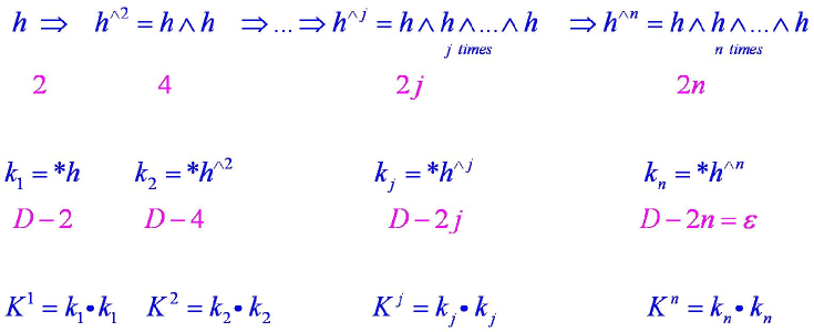
Figure 3: Killing-Yano tower

The first row of this diagram contains external powers ${\mbox{\boldmath$h$}}^{\wedge k}$ of the principal CKY tensor, which again are closed CKY tensors. Taking the Hodge dual of these tensors one obtains a set of Killing-Yano tensors ${\mbox{\boldmath$k$}}_{i}$. ‘Squares’ of ${\mbox{\boldmath$k$}}_{i}$ give a set of second rank Killing tensors ${\mbox{\boldmath$K$}}^{i}$. For even $D$ the last column can be omitted since ${\mbox{\boldmath$h$}}^{\wedge n}$ is proportional to a totally antisymmetric tensor, and hence it does not produce a non-trivial Killing tensor. For the odd case, the Killing tensor ${\mbox{\boldmath$K$}}^{n}$ is a product of two Killing vectors and hence it is reducible. The first $n-1$ Killing tensors are irreducible. The metric itself is also a Killing tensor, ${\mbox{\boldmath$K$}}^{0}={\mbox{\boldmath$g$}}$. We call the Killing-Yano tower extended if the metric is included into it. Thus the extended Killing-Yano tower allows one to construct $n$ independent quadratic in momenta conserved quantities for a geodesic motion.

Besides a tower of the rank 2 Killing tensors, the principal CKY tensor generates a set of the Killing vectors. To demonstrate this let us notice that for a CKY tensor $h$ of rank-$2$ the vector

$$\xi^{(0)a}={1\over D-1}\nabla_{b}h^{ab}$$ (31)

obeys the following equation [40, 45]

$$\xi^{(0)}_{\ (a;b)}=-{1\over D-2}R_{c(a}h_{b)}^{\,\,\,\,c}\,.$$ (32)

Thus, in an Einstein space, that is when $R_{ab}=\Lambda g_{ab}$, ${\mbox{\boldmath$\xi$}}^{(0)}$ is the Killing vector. It can be shown that even if the Einstein equations with the cosmological constant are not imposed the vector $\xi^{(0)a}$ constructed for the principal CKY tensor is always the Killing vector[46]. We call it a primary Killing vector. Acting by the Killing tensors ${\mbox{\boldmath$K$}}^{i}$ on the primary Killing vector one obtains a set of the independent commuting Killing vectors[43, 46, 47]

$$\xi^{i}_{a}=K^{i}_{ab}\xi^{(0)b}\,.$$ (33)

There Killing vectors (with an additional Killing vector ${\mbox{\boldmath$k$}}_{n}$ for $\varepsilon=1$) give $n+\varepsilon$ conserved first order in momentum quantities for the geodesic motion. These conserved quantities together with $n-$ conserved quantities connected with the Killing tensors (including the metric $g$) form a set of $D=2n+\varepsilon$ conserved quantities.

5 Darboux basis

Let us consider an eigenvalue problem for a conformal Killing tensor $H$ associated with $h$

$$H_{ab}\equiv h_{ac}h_{b}^{\ \,c}\,.$$ (34)

It is easy to show that in the Euclidean domain its eigenvalues $x^{2}$,

$$H^{a}_{\ b}v^{b}=x^{2}v^{a}\,,$$ (35)

are real and non-negative. Using a modified Gram–Schmidt procedure it is possible to show that there exists such an orthonormal basis in which the operator $h$ has the following structure:

$$\mbox{diag}({\mbox{\boldmath$0$}},{\mbox{\boldmath$\Lambda$}}_{1},\ldots,{\mbox{\boldmath$\Lambda$}}_{p})\,,$$ (36)

where ${\mbox{\boldmath$\Lambda$}}_{i}$ are matrices of the form

$$\Lambda_{i}=\left(\begin{array}[]{cc}0&-x_{i}{\mbox{\boldmath$I$}}\\ x_{i}{\mbox{\boldmath$I$}}&0\end{array}\right)\,,$$ (37)

$\mathrm{𝟎}$ is a zero matrix and $I$ are unit matrices. For a non-degenerate principal CKY tensor $h$ the eigenspaces corresponding to the eigenvalues $x_{i}$ are two dimensional (Darboux subspaces). Since the matrix rank of $h$ is $2n$ the eigenvalue $0$ is present only for $\varepsilon=1$, and the corresponding eigenspace in this case is one dimensional. We assume also that $h$ is non-degenerate, that is $p=n$ and the eigenspaces of $H$ are two-dimensional so that the matrices $\Lambda$ has the form

$$\Lambda_{i}=\left(\begin{array}[]{cc}0&-x_{i}\\ x_{i}&0\end{array}\right)\,.$$ (38)

(See Section 9 for a discussion of a degenerate case.)

We denote by ${\mbox{\boldmath$e$}}_{\hat{\mu}}$ and ${\mbox{\boldmath$\tilde{e}$}}_{\hat{\mu}}\equiv{\mbox{\boldmath$e$}}_{\hat{n}+\hat{\mu}}$, where $\mu=1,\ldots,n$, mutually orthogonal unit vectors in the 2D Darboux space corresponding to the eigenvalue $x_{\mu}$. For $\varepsilon=1$ we introduce also a unit vector ${\mbox{\boldmath$e$}}_{\hat{0}}$ in the subspace corresponding to zero eigenvalue. The basis of the dual forms we denote by ${\mbox{\boldmath$\omega$}}^{\hat{\mu}}$ and ${\mbox{\boldmath$\tilde{\omega}$}}^{\hat{\mu}}\equiv{\mbox{\boldmath$\omega$}}^{\hat{n}+\hat{\mu}}$ (and ${\mbox{\boldmath$\omega$}}^{\hat{0}}$ if $\varepsilon=1$). The metric $g$ and the principal CKY tensor $h$ in this basis take the form

$$g = =\sum_{\mu=1}^{n}({\mbox{\boldmath$\omega$}}^{\hat{\mu}}{\mbox{\boldmath$\omega$}}^{\hat{\mu}}+{\mbox{\boldmath$\tilde{\omega}$}}^{\hat{\mu}}{\mbox{\boldmath$\tilde{\omega}$}}^{\hat{\mu}})+\varepsilon{\mbox{\boldmath$\omega$}}^{\hat{0}}{\mbox{\boldmath$\omega$}}^{\hat{0}}\,,$$ (39)

$$h = \!\!\sum_{\mu=1}^{n}x_{\mu}{\mbox{\boldmath$\omega$}}^{\hat{\mu}}\wedge{\mbox{\boldmath$\tilde{\omega}$}}^{\hat{\mu}}\,.$$ (40)

Starting with the principal CKY tensor $h$ written in the canonical form, one can find the explicit expressions for the other associated tensors of the Killing tower. In particular, for the associated Killing tensors one has

$${\mbox{\boldmath$K$}}^{(j)} = \sum_{\mu=1}^{n}A^{(j)}_{\mu}({\mbox{\boldmath$\omega$}}^{\hat{\mu}}{\mbox{\boldmath$\omega$}}^{\hat{\mu}}+{\mbox{\boldmath$\tilde{\omega}$}}^{\hat{\mu}}{\mbox{\boldmath$\tilde{\omega}$}}^{\hat{\mu}})+\varepsilon A^{(j)}{\mbox{\boldmath$\omega$}}^{\hat{0}}{\mbox{\boldmath$\omega$}}^{\hat{0}}\,$$ (41)

$$A^{(j)}\!\! = \!\!\sum_{\nu_{1}<\dots<\nu_{j}}\!x_{\nu_{1}}^{2}\dots x_{\nu_{j}}^{2}\;,\quad A^{(j)}_{\mu}=\!\!\sum_{{\nu_{1}<\dots<\nu_{j}\atop\nu_{i}\neq\mu}}\!x_{\nu_{1}}^{2}\dots x_{\nu_{j}}^{2}\,.$$ (42)

It should be emphasized that Killing tensors are defined up to an arbitrary constant factor. In order to obtain the above expressions this factors were specially chosen, so that ${\mbox{\boldmath$K$}}^{(j)}$ in Eq.(41) contains an extra constant factors with respect to ${\mbox{\boldmath$K$}}^{j}$ from the diagram 3 for the Killing tower.

6 Canonical form of the metric

In the presence of the principal CKY tensor, one can use its independent eigenvalues $x_{i}$ as $n$ coordinates. Moreover, the principal CKY tensor generates $n+\varepsilon$ Killing vectors, one primary $\xi^{(0)}$, Eq.(31), and $n-1+\varepsilon$ secondary $\xi^{(i)}$, defined by Eq.(33) with ${\mbox{\boldmath$K$}}^{i}$ substituted by ${\mbox{\boldmath$K$}}^{(i)}$, ones. Denote by $\psi_{0}$ and $\psi_{i}$ the corresponding Killing parameters,

$$\xi^{(0)}=\partial_{\psi_{0}}\,,\hskip 14.22636pt\xi^{(i)}=\partial_{\psi_{i}}\,.$$ (43)

A set of $n$ essential (Darboux) coordinates $x_{i}$ and $n+\varepsilon$ Killing coordinates $\{\psi_{0},\psi_{i}\}$ can be used as $D=2n+\varepsilon$ coordinates associated with the principal CKY tensor. We call these coordinates canonical. It can be shown that the metric of a spacetime, which admits a principal CKY tensor, can be written in the canonical coordinates in the form

$${\mbox{\boldmath$\omega$}}^{\hat{\mu}} = \frac{1}{\sqrt{Q_{\mu}}}\,dx_{\mu}\,,\hskip 5.69046pt{\mbox{\boldmath$\tilde{\omega}$}}^{\hat{\mu}}=\sqrt{Q_{\mu}}\,\sum_{k=0}^{n-1}A^{(k)}_{\mu}\,d\psi_{k}\,,\hskip 5.69046pt{\mbox{\boldmath$\omega$}}^{0}=(-c/A^{(n)})^{1/2}\sum_{k=0}^{n}A^{(k)}{\mbox{\boldmath$d$}}\psi_{k}\,,$$ (44)

$$Q_{\mu} = X_{\mu}/U_{\mu}\,,\quad U_{\mu}=\prod_{\nu\neq\mu}(x_{\nu}^{2}-x_{\mu}^{2})\,.$$ (45)

This result was first proved in [49] assuming the the following two conditions

$${\cal L}_{\xi}{\mbox{\boldmath$g$}}=0\,,\hskip 14.22636pt{\cal L}_{\xi}{\mbox{\boldmath$h$}}=0\,,$$ (46)

where $\xi$ is defined by Eq.(30), are satisfied. Later it was shown [46] that these conditions follow from the very existence of the principal CKY tensor and the canonical form was derived in a general case for a spacetime with the principal CKY tensor [46, 50]. Here $A^{(k)}_{\mu}$ and $A^{(k)}$ are given by Eq.(42), and $X_{\mu}$ are functions of a single argument $x_{\mu}$. It should be emphasized that in the derivation of this form of the metric the Einstein equations were not used. In this sense, this is an off-shell result.

By imposing the $D$-dimensional Einstein equations with a cosmological constant one obtains that the functions $X_{\mu}$ are of the form

$$X_{\mu}=\sum\limits_{k=\varepsilon}^{n}c_{k}x_{\mu}^{2k}-2b_{\mu}x_{\mu}^{1-\varepsilon}+\frac{\varepsilon c}{x_{\mu}^{2}}\,.$$ (47)

‘Time’ is denoted by $\psi_{0}$, azimuthal coordinates by $\psi_{k}$, ${k=1,\dots,m=n-1+\varepsilon}$, and ${x_{\mu}}$, ${\mu=1,\dots,n}$, stand for ‘radial’ and latitude coordinates. The physical metric with proper signature is recovered when standard radial coordinate $r=-ix_{n}$ and new parameter $M=(-i)^{1+\epsilon}b_{n}$ are introduced. The total number of constants which enter the solution is $2n+1$: $\varepsilon$ constants $c$, $n+1-\varepsilon$ constants $c_{k}$ and $n$ constants $b_{\mu}$. The form of the metric is invariant under a 1-parameter scaling coordinate transformations, thus a total number of independent parameters is $D-\varepsilon$. These parameters are related to the cosmological constant, mass, angular momenta, and NUT parameters. One of them may be used to define a scale, while the other $D-1-\varepsilon$ parameters can be made dimensionless. (For more details see [12].) In the absence of NUT parameters and for vanishing cosmological constant the metric Eq.(44)-Eq.(47) reduces to the Myers-Perry metric describing an isolated rotating higher dimensional black hole in an asymptotically flat spacetime. The existence of the closed CKY tensor for Myers-Perry [51] and Kerr-NUT-(A)dS was established first in [35, 36], where it was also demonstrated that the corresponding principal CKY tensor does not depend on the parameters of the solution (universality property).

7 Separation of variables

The Hamilton-Jacobi equation for geodesic motion

$${\partial S\over\partial\lambda}+g^{ab}\partial_{a}S\partial_{a}S=0\,,$$ (48)

in the Kerr-NUT-(A)dS spacetime allows a complete separation of variables [52]

$$S=-w\lambda+\sum_{k=0}^{n+\varepsilon-1}\Psi_{k}\psi_{k}+\sum_{\mu=1}^{n}S_{\mu}(x_{\mu})\,.$$ (49)

The functions $S_{\mu}$ obey the first order ordinary differential equations

$${S^{\prime}_{\mu}}^{2}={V_{\mu}\over X_{\mu}}-{W_{\mu}^{2}\over X_{\mu}^{2}}\,,$$ (50)

Here

$$W_{\mu}=\sum_{k=0}^{n+\varepsilon-1}\Psi_{k}(-x_{\mu}^{2})^{n-1-k}\,,\hskip 5.69046ptV_{\mu}=\sum_{k=0}^{n+\varepsilon-1}\kappa_{k}(-x_{\mu}^{2})^{n-1-k}\,.$$ (51)

For $\varepsilon=1$ we put $\kappa_{n}=\Psi_{n}^{2}/c$. The parameters $\kappa_{k}$ and $\Psi_{k}$ are separation constants. The existence of $D$ independent conserved constants which enter these functions implies a complete integrability of the geodesic motion equations in the spacetimes admitting the principal CKY tensor (for more details, see [43, 44]).

Similarly, the massive scalar field equation

$$\Box\Phi-\mu^{2}\Phi=0\,,$$ (52)

in the Kerr-NUT-(A)dS metric allows a complete separation of variables [52]. Namely, the solution can be decomposed into modes

$$\Phi=\prod_{\mu=1}^{n}R_{\mu}(x_{\mu})\prod_{k=0}^{n+\varepsilon-1}e^{i\Psi_{k}\psi_{k}}\,.$$ (53)

Substitution of Eq.(53) into the equation Eq.(52) results in the following second order ordinary differential equations for functions $R_{\mu}(x_{\mu})$

$$(X_{\mu}R^{\prime}_{\mu})^{\prime}+\varepsilon{X_{\mu}\over x_{\mu}}R^{\prime}_{\mu}+\left(V_{\mu}-{W_{\mu}^{2}\over X_{\mu}}\right)R_{\mu}=0\,.$$ (54)

Here $W_{\mu}$ and $V_{\mu}$ are given by Eq.(51) and $\kappa_{0}=-\mu^{2}$

In [53] it was shown that the following operators

$${\hat{\xi}}_{(k)} = -i\xi^{(k)a}\partial_{a}\,,\quad k=0,\ldots,m\,,$$ (55)

$${\hat{K}}_{(j)} = -{1\over\sqrt{|g|}}\,\partial_{a}\Bigl{(}\sqrt{|g|}K^{(j)\,\!ab}\partial_{b}\Bigr{)}\,,\quad j=0,\ldots,n-1\,,$$ (56)

determined by a principal CKY tensor, form a complete set of commuting operators for the Klein–Gordon equation in the Kerr-NUT-(A)dS background.

Using Eq.(56) one has ${\hat{K}}_{(0)}=-\Box$. Since all the operators Eq.(55)–Eq.(56) commute with one another, their common eigenvalues can be used to specify the modes. It is possible to show [53] that the eigen-vectors of these commuting operators are the modes Eq.(53) and one has

$${\hat{\xi}}_{(k)}\Phi=\Psi_{k}\Phi\,,\quad{\hat{K}}_{(j)}\Phi=\kappa_{j}\Phi\,.$$ (57)

Later it was shown that the massive Dirac equation in the Kerr-NUT-(A)dS spacetime also allows the separation of variables [54]. More recently Oota and Yasui [55] demonstrated separability of the tensor type gravitational perturbations in a (generalized) Kerr-NUT-(A)dS spacetime. It was also proved that the stationary test string equations in the Kerr-NUT-(A)dS spacetime are completely integrable [56] .

8 Parallel transport of frames along geodesics

One of the additional remarkable properties of the 4D Kerr metric, discovered by Marck in 1983 [57, 58, 59], is that the equations of parallel transport can be integrated. This result allows a generalization: In a higher dimensional spacetime which admits a principal CKY tensor equations of a parallel-propagated frame along a geodesic can be solved explicitly [60, 61].

The main idea of this construction is the following. Let $u$ be a tangent vector to a geodesic. Consider a 2-form $F$ which is obtained by projecting $h$ onto a subspace $V$ orthogonal to $u$

$$F_{ab}=P_{a}^{c}P_{b}^{d}h_{cd}=h_{ab}+u_{a}u^{c}h_{cb}+h_{ac}u^{c}u_{b}\,,$$ (58)

where ${P_{a}^{b}=\delta_{a}^{b}+u^{b}u_{a}}$ is the projector onto $V$. This form $F$ can be also written as follows

$$F = -{\mbox{\boldmath$u$}}\raisebox{-1.50696pt}{\makebox[6.00006pt][r]{\scriptsize$-$}}\raisebox{1.07639pt}{\makebox[3.99994pt][l]{\tiny$|$}}({\mbox{\boldmath$u$}}^{\flat}\wedge{\mbox{\boldmath$h$}})={\mbox{\boldmath$h$}}+{\mbox{\boldmath$u$}}^{\flat}\wedge{\mbox{\boldmath$s$}}\,,$$ (59)

$$s = {\mbox{\boldmath$u$}}\raisebox{-1.50696pt}{\makebox[6.00006pt][r]{\scriptsize$-$}}\raisebox{1.07639pt}{\makebox[3.99994pt][l]{\tiny$|$}}{\mbox{\boldmath$h$}}\,,\hskip 14.22636pts_{b}=u^{a}h_{ab}\,.$$ (60)

Let us demonstrate that $F$ is parallel propagated along a geodesic. The definition Eq.(30) of the principal CKY tensor implies

$$\nabla_{u}{\mbox{\boldmath$h$}}={\mbox{\boldmath$u$}}^{\flat}\wedge{\mbox{\boldmath$\xi$}}^{\flat}\,.$$ (61)

Hence

$$\nabla_{u}({\mbox{\boldmath$u$}}^{\flat}\wedge{\mbox{\boldmath$h$}})={\mbox{\boldmath$u$}}^{\flat}\wedge\nabla_{u}{\mbox{\boldmath$h$}}={\mbox{\boldmath$u$}}^{\flat}\wedge{\mbox{\boldmath$u$}}^{\flat}\wedge{\mbox{\boldmath$\xi$}}^{\flat}=0\,.$$ (62)

Thus for a geodesic motion, $\nabla_{u}{\mbox{\boldmath$u$}}=0$, the 2-form $F$ is parallel propagated along the geodesic [44].

The 2-form $F$ has its own Darboux basis, which is called comoving. For any geodesic the comoving basis is determined along its trajectory. Since $F$ is parallel propagated, its eigenvalues and its Darboux subspaces, which are called the eigenspaces of $F$, are parallel-transported. For a generic timelike (or spacelike) geodesic the eigenspaces of $F$ are at most 2-dimensional. In fact, the eigenspaces with non-zero eigenvalues are 2-dimensional, and the zero-value eigenspace is 1-dimensional for odd number of spacetime dimensions and 2-dimensional for even. So, the comoving basis is defined up to rotations in each of the 2D eigenspaces. The parallel-propagated basis is a special comoving basis. It can be found by solving a set of the first order ordinary differential equations for the angles of rotation in the 2D eigenspaces. It is possible to show that these ordinary differential equations can be solved by means of separation of variables [60]. A modification of this procedure can be used to construct parallel propagated frames along null geodesics [61].

9 Degenerate case

Consider a closed rank-$2$ CKY tensor $h$ and denote by $x_{\mu}$ ($\mu=1,\cdots,n$) and $\xi_{i}$ ($i=1,\cdots,N$) its non-constant eigenvalues and the non-zero constant ones, respectively. Suppose the eigenvalues of the “square of the CKY tensor” $H=(H^{a}{}_{b})=(-h^{a}{}_{c}h^{c}{}_{b})$ have the following multiplicities:

$$\{\underbrace{x_{1}^{2},\dotsm,x_{1}^{2}}_{2\ell_{1}},\dotsm,\underbrace{x_{n}^{2},\dotsm,x_{n}^{2}}_{2\ell_{n}},\underbrace{\xi_{1}^{2},\dotsm,\xi_{1}^{2}}_{2m_{1}},\dotsm,\underbrace{\xi_{N}^{2},\dotsm,\xi_{N}^{2}}_{2m_{N}},\underbrace{0,\dotsc,0}_{K}\},$$ (63)

where $D=2(|\ell|+|m|)+K$. Here $|\ell|=\sum_{\mu=1}^{n}\ell_{\mu}$ and $|m|=\sum_{i=1}^{N}m_{i}$. In the previous consideration we assumed that the principal CKY tensor $h$ is non-degenerate, that is

$$\ell_{1}=\ldots=\ell_{n}=1\,,\hskip 14.22636ptm_{1}=\ldots=m_{N}=0\,,\hskip 14.22636ptK=\varepsilon\,.$$ (64)

If these conditions are violated we call a principal CKY tensor degenerate. Recently there was obtained a general canonical form of a spacetime which admits a degenerate principal CKY tensor [47, 62]. These papers also contain a generalized Kerr-NUT-(A)dS metrics which are solutions of the higher dimensional Einstein equations with a cosmological constant with a arbitrary degenerate principal CKY tensor. It is interesting to notice that a 4D Taub-NUT metric belongs to this class of the solutions. An example of a generalized Kerr-NUT-(A)dS with a degenerate principal CKY tensor is a special subclass of Kerr-(A)dS solutions [63, 64]. In a general case these solutions contain $[(D-1)/2]$ different angular momenta. In the case when some of them are equal, the principal CKY tensor has constant eigenvalues [55].

At the moment not so much is known about properties and interpretation of the generalized Kerr-NUT-(A)dS solutions in higher dimensions.

10 Concluding remarks

During past 2-3 years a lot of important and interesting results concerning higher dimensional black hole solutions with the spherical topology of the horizon were obtained. It was discovered that a key role in this study is played by the principal CKY tensor. The very existence of this tensor in a spacetime restricts the form of the metric. In the non-degenerate case this canonical metric obeying the Einstein equations coincides with the Kerr-NUT-(A)dS solution. The class of metrics admitting a principal CKY tensor allows separation of variables in the Hamilton-Jacobi, Klein-Gordon, Dirac, and tensor perturbation. It is still an open question whether other massless fields equations, e.g. the Maxwell field, allow separation of variables in the (generalized) Kerr-NUT-(A)dS spacetime. Another interesting question concerns a possibility to separate variables in the higher dimensional spacetimes in the absence of the principal CKY tensor. It may happen when such a space admits a sufficient number of commuting Killing vectors and Killing tensors [65]. Especially, this problem of separation of variables is important for study black ring and black saturn solutions. Separation of variables for the gravitational perturbations is important for the analysis of the stability of these higher dimensional solutions. Another interesting direction of research is study of the hidden symmetries in supergravity black holes (see e.g. [67]) and, more generally, study of the relation between hidden symmetries and supersymmetry.

References

- [1] Arkani-Hamed N, Dimopoulos S and Dvali G.R. 1998 Phys. Lett. B 429 263
- [2] Antoniadis I, Arkani-Hamed N, Dimopoulos S and Dvali G.R. 1998 Phys. Lett. B 436 257
- [3] Randall L and Sundrum R 1999 Phys. Rev. Lett. 83 3370
- [4] Randall L and Sundrum R 1999 Phys. Rev. Lett. 83 4690
- [5] Giddings, S B 2007 AIP Conf.Proc. 957 69 e-Print: arXiv:0709.1107
- [6] Kanti P 2004 Int. J. Mod. Phys. A 19 4899
- [7] Kanti P 2007 e-Print: arXiv:0802.2218
- [8] Park S C 2008 e-Print: arXiv:0809.2571
- [9] Emparan R and Real H S 2002 Phys. Rev. Lett. 88 101101
- [10] Elvang H and Figueras P 2007 JHEP 0705 050
- [11] Emparan R and Real H S 2008 e-Print arXiv:0801.3471
- [12] Chen W, Lü H and Pope C N 2006 Class. Quantum Grav. 23 5323
- [13] Hamamoto N, Houri T, Oota T and Yasui Y 2007 Journ. Phys. A 40 F177
- [14] Milson R, Coley A, Pravda V and Pravdová A 2005 Int. J. Geom. Meth. Mod. Phys. 2 41
- [15] Coley A, Milson R, Pravda V and Pravdová A 2004 Class. Quantum Grav. 21 L35
- [16] Coley A 2008 Class. Quantum Grav. 25 033001
- [17] Carter B 1968 Phys. Rev. 174 1559
- [18] Carter B 1968 Commun. Math. Phys. 10 280
- [19] Walker M and Penrose R 1970 Commun. Math. Phys. 18 265
- [20] Penrose R 1973 Ann. N. Y. Acad. Sci. 224 125; Floyd R 1973 The dynamics of Kerr fields, PhD Thesis, London
- [21] Yano K 1952 Ann. Math. 55 328
- [22] Collinson C D 1976 Int. J. Theor. Phys. 15 311; Stephani H 1977 Gen. Rel. Grav. 9 789; Ferrando J J and Sáez J A 2002 Gen. Rel. Grav. 35 1191
- [23] Collinson C D 1974 Tensor 28 173
- [24] Kinnersley W 1969 J. Math. Phys. 10 1195
- [25] Demianski M and Francaviglia M 1980 Int. J. Theor. Phys. 19 675
- [26] Dietz W and Rüdiger R 1981 Proc. R. Soc. A 375 361; Dietz W and Rüdiger R 1982 Proc. R. Soc. A 381 315
- [27] Teukolsky S A 1972 Phys. Rev. Lett. 29 1114
- [28] Unruh W 1973 Phys. Rev. Lett. 31 1265
- [29] Teukolsky S A 1973 Astrophys. J. 185 635
- [30] Chandrasekhar S 1976 Proc. Roy. Soc. London A349 571
- [31] Page D N 1976 Phys. Rev. D 14 1509
- [32] Frolov V P and Stojkovic D 2003 Phys. Rev. D 67 084004
- [33] Frolov V P and Stojkovic D 2003 Phys. Rev. D 68 064011
- [34] Gooding and Frolov A V 2008 Phys. Rev. D 77 104026
- [35] Frolov V P and Kubizňák D \PRL982007011101
- [36] Kubizňák D and Frolov V P \CQG242007F1
- [37] Frolov V 2008 Prog. Theor. Phys. Suppl. 172 210
- [38] Frolov V and Kubizňák D 2008 Class. Quantum Grav. 25 154005
- [39] Kubizňák D 2008 e-Print: arXiv:0809.2452
- [40] Tachibana S 1969 Tôhoku Math. J. 21 56; Kashiwada T 1968 Nat. Sci. Rep., Ochanomizu University 19 67
- [41] Benn I M, Charlton P and Kress J 1997 J. Math. Phys. 38 4504
- [42] Kress J 1997 Generalized Conformal Killing-Yano Tensors: Applications to Electrodynamics, PhD Thesis, University of Newcastle
- [43] Krtouš P, Kubizňák D, Page D N and Frolov V P 2007 J. High Energy Phys. 02 004
- [44] Page D N, Kubizňák D, Vasudevan M and Krtouš P 2007 Phys. Rev. Lett. 98 061102
- [45] Jezierski J 1997 Class. Quantum Grav. 14 1679
- [46] Krtouš P, Frolov V P , Krtouš P 2008 e-Print: arXiv:0804.4705
- [47] Houri T, Oota T and Yasui Y 2008 J. Phys. A 41 025204
- [48] Carter B 1968 Phys. Lett. A 26 399
- [49] Houri T, Oota T and Yasui Y 2007 Phys. Lett. B 656 214
- [50] Houri T, Oota T and Yasui Y 2008 Phys. Lett. B 666 391
- [51] Myers R C and Perry M J 1986 Ann. Phys. (N.Y.) 172 304
- [52] Frolov V P, Krtouš P and Kubizňák D 2007 J. High Energy Phys. 02 005
- [53] Sergyeyev A and Krtouš P 2008 Phys. Rev. D 77 044033
- [54] Oota T and Yasui Y 2008 Phys. Lett. B 659 688
- [55] Oota T and Yasui e-Print: arXiv:0812.1623 (2008)
- [56] Kubizňák D and Frolov V P 2008 JHEP 0802 007
- [57] Marck J A 1983 Proc. R. Soc. A 385 431
- [58] Marck J A 1983 Phys. Lett. B 97 140
- [59] Kamran N and Marck J A 1986 J. Math. Phys. 27 1589
- [60] Connell P, Frolov V and Kubizňák D 2008 Phys. Rev. D 78 024042
- [61] Kubizňák D, Frolov V, Krtouš, and Connell P arXiv:0809.2452v1 [gr-qc], 2008
- [62] Houri T, Oota T and Yasui Y 2008 e-Print: arXiv:0805.3877
- [63] Gibbons G W, Lu H, Page D, Pope C N 2004 Phys. Rev. Lett. 93 171102
- [64] Gibbons G W, Lu H, Page D, Pope C N 2005 J.Geom.Phys. 53 49
- [65] Benenti S and Francaviglia M 1979 Gen. Rel. Grav. 10 79
- [66] Hoskisson J 2008 Phys. Rev. D 78 064039
- [67] Chow D D K 2008 e-Print: arXiv:0811.1264