Fermionic propagators for 2D systems with singular interactions

Abstract

We analyze the form of the fermionic propagator for 2D fermions interacting with massless overdamped bosons. Examples include a nematic and Ising ferromagnetic quantum-critical points, and fermions at a half-filled Landau level. Fermi liquid behavior in these systems is broken at criticality by a singular self-energy, but the Fermi surface remains well defined. These are strong-coupling problems with no expansion parameter other than the number of fermionic species, $N$. The two known limits, $N>>1$ and $N=0$ show qualitatively different behavior of the fermionic propagator $G(\epsilon_{k},\omega)$. In the first limit, $G(\epsilon_{k},\omega)$ has a pole at some $\epsilon_{k}$, in the other it is analytic. We analyze the crossover between the two limits. We show that the pole survives for all $N$, but at small $N$ it only exists in a range $O(N^{2})$ near the mass shell. At larger distances from the mass shell, the system evolves and $G(\epsilon_{k},\omega)$ becomes regular. At $N=0$, the range where the pole exists collapses and $G(\epsilon_{k},\omega)$ becomes regular everywhere.

I Introduction

Physical properties of fermionic systems interacting with critical neutral fluctuations have been a focus of intense studies over the last several decades and yet remain a subject of advanced research. Examples include fermions interacting with a gauge field, Lee ; AIM a half-filled Landau level, AIM ; senthil and the system behavior at quantum-critical points (QCP) towards Ising-type ferromagnetism Chubukov04 ; Chubukov06 ; Dzero (FM) and towards a nematic order.Oganesyan ; Lawler ; MRA ; Kee The later case is an example of a Pomeranchuk-type Fermi surface instability of an isotropic Fermi liquidPom1 . In all such systems, scattering of fermions by massless bosonic excitations leads to a non-analytic form of the fermionic self-energy $\Sigma(k,\omega_{m})$. Below the upper critical dimension $D_{cr}$, $\Sigma(k_{\text{\tiny{F}}},\omega_{m})$ exceeds a bare $i\omega_{m}$ term in the fermionic propagator, and the system develops a non-Fermi liquid behavior. At a critical point towards a nematic or an Ising ferromagnet, one-loop self-energy $\Sigma(k_{\text{\tiny{F}}},\omega_{m})\propto i\omega_{m}^{D/3}$, and $D_{cr}=3$ (Ref. Lee, ). The singular behavior of the self-energy is, however, only in the frequency domain, the momentum dependence of $\Sigma(k,0)$ remains regular: $\Sigma(k,0)\propto\epsilon_{k}$. As a consequence, the Fermi surface remains well defined at $k_{\text{\tiny{F}}}$ as a locus of singular points of $G({\bf k},0)$ despite that Landau quasiparticles do not exist.

In 2D, one-loop self-energy $\omega^{D}_{m}$ becomes $\omega^{2/3}_{m}$. It has long been the issue AIM ; Khvesh ; Chubukov06 ; Lawler ; CK06 whether $\omega^{2/3}_{m}$ form is the exact expression for a non-Fermi liquid fermionic propagator. The answer to this question is still lacking. On one hand, the two-loop and higher order self-energies also scale as $\omega_{m}^{2/3}$, i.e., the exponent remains the same to all orders. On the other hand, higher-order terms are of the same order as one-loop self-energy, and it is a’priori unclear what the sum of infinite series of $\omega_{m}^{2/3}$ terms yields.

The way to treat such systems in a controlled way is to artificially extend them to $N$ fermionic flavors and require that the interaction with a boson conserves the flavor. At large $N$, multi-loop $\omega_{m}^{2/3}$ self-energy terms acquire extra powers of $(\ln N/N)^{2}$ and the series of $\omega_{m}^{2/3}$ terms converge. In this situation, self-energy is essentially determined by the one-loop term $\Sigma(k,\omega_{m})=i|\omega_{m}|^{2/3}\omega^{1/3}_{0}\operatorname{sgn}(\omega_{m})$, where $\omega_{0}$ is the internal energy scale. Accordingly, at $\omega_{m}>0$ which we only consider below,

$$G({\bf k},\omega_{m}) \approx \frac{1}{i\omega^{2/3}_{m}\omega^{1/3}_{0}-\epsilon_{k}}$$

$$= -\frac{1}{\epsilon_{k}}F_{N\to\infty}\left(-\frac{\omega^{2/3}_{m}\omega^{1/3}_{0}}{\epsilon_{k}}\right),$$

$$F_{N\to\infty}(x) = \frac{1}{1+ix}.$$ (1)

As a function of a complex $x$, $F_{N\rightarrow\infty}(x)$ has a simple pole at $x=i$. Because of the pole, real space/time propagator $G({\bf r},t)$ is long-ranged and decays by a power-law, as $G({\bf r},t=0)\propto 1/r^{2}$ and $G(v_{F}t>>{\bf r})\propto 1/(t\sqrt{r})$. (see Appendix A).

Another solvable limit is $N=0$. In this case the curvature of the 2D Fermi surface scales out, the system behavior becomes effectively one-dimensional and can be obtained by bosonization. The Green’s function at $N=0$ has been obtained by Ioffe et al  Lidsky and Altshuler et al. AIM It is still given by Eq. (1), but the functional form of $F_{N=0}(x)$ is fundamentally different: $F_{N=0}(x)$ is analytic in any finite region in the upper half-plane of $x$ and becomes singular only at $x=\infty$. Because the pole is absent, $G({\bf r},t)$ is now short-ranged and at $v_{\text{\tiny{F}}}t\gg r$ scales as $G({\bf r},t)\propto\left[1/t\sqrt{r}\right]\exp[-ar/t^{2/3}]$, where $a$ is a dimensional prefactor.

Different behavior of $F_{N}(x)$ at large $N$ and at $N=0$ raises the question which of the two forms (if any) describes system behavior in the physical case of $N=1$. Altshuler et al conjectured AIM that the $N=0$ case is special, and the system behavior at any $N\neq 0$ is qualitatively the same as for large $N$, i.e., the pole in $F_{N}$ persists for all $N$ and only vanishes at $N=0$. On the contrary, Fradkin and Lawler Lawler argued that exponential behavior of $G({\bf r},t)$ survives at finite $N$. One of us and Khveshchenko argued CK06 that the curvature of a 2D Fermi surface is relevant for any $N>0$, and $G({\bf r},t)$ decays by a power-law once $N>0$. However, the calculations in Ref. CK06, are approximate and did not yield the same $G({\bf r},t=0)\propto 1/r^{2}$ as at $N\rightarrow\infty$.

In this paper, we analyze this issue in detail by performing loop expansion at small $N$. We find, in agreement with the conjecture by Altshuler et al  AIM that the pole in the Green’s function exists at any finite $N$, and real-space, equal time Green’s function $G(r,t=0)$ decays by a power-law, as $1/r^{2}$. The way how the pole disappears at $N\rightarrow 0$ is, however, somewhat counter-intuitive. Naively, one could expect that the residue of the pole $Z_{N}$ gradually vanishes as $N\rightarrow 0$. We, however, found a different behavior: the residue $Z_{N}$ remains $O(1)$ at small $N$, but the pole only exists in the range $\Delta<N^{2}$, where $\Delta$, introduced in (2) below, is the distance from the pole. Outside this range, the Green’s function is regular and the same as at $N=0$. At $N\rightarrow 0$, the range collapses and the Green’s function becomes regular even at $\Delta=0$.

We present computational details below, but first summarize our rational. As our primary goal is to study what happens at small but finite $N$, we cannot use bosonization, which is only applicable at $N=0$, and have to rely on the diagrammatic loop expansion. It is not guaranteed a’priori that loop expansion is useful at small $N$ as all terms in the series are generally of the same order, and it could be the case that the corrections are all regular near the mass shell, but the prefactors are arranged such that infinite series of regular $O(1)$ corrections to the quasiparticle residue diverge at $N=0$ and destroy the pole.

We, however, found that the actual situation is different, and the the pole disappears at $N=0$ and is still present at a finite $N$ not because regular series diverge (at $N=0$) or almost diverge (at $N>0$), but because of a peculiar singularity in the self-energy, whose form is different at $N=0$ and at finite $N$. This singularity can be captured within the loop expansion. Specifically, we find that the expansion of the self-energy $\Sigma$ near the mass shell, in powers of

$$\Delta=1-\frac{i}{x}=1+i\frac{\epsilon_{k}}{\omega^{2/3}_{m}\omega^{1/3}_{0}}$$ (2)

contains a universal term which is “non-perturbative” in the sense that it comes from fermions whose energies are of order $\omega\Delta^{3/2}$, which are smaller than the external energy $\omega$. This term appears at the two-loop order and at $N=0$ yields the non-analytic contribution to the self-energy which scales as $\Delta^{3/2}$. At a first glance, such term cannot eliminate a pole as it is smaller than $G^{-1}_{0}=\Delta$. However, this universal self-energy gets renormalized by logarithmically divergent vertex corrections, which, because typical energies scale with $\Delta$, are powers of $\ln\Delta$. Series of such corrections exponentiate into the full vertex $\Gamma\propto\Delta^{-a}$ and modify the universal self-energy to $\Delta^{3/2}\Gamma^{2}\sim\Delta^{3/2-2a}$. The exponent $a=1$ in the leading logarithmical approximation (when only the highest power of the logarithm is kept at any order), but gets renormalized by $O(1)$ corrections beyond this approximation. We cannot find $a$ explicitly, but a comparison with bosonization implies that $a=3/4$ in which case the fully renormalized self-energy tends to a constant value on the mass shell, i.e., the pole in $G(k,\omega)$ disappears.

We next turn to $N>0$. We found that universal contribution to the self-energy do exist in this case as well, but at the smallest $\Delta<<N^{2}$ it behaves as $\Delta^{5}/N^{2}$ (up to extra logarithms) Because typical internal energies are still small, vertex corrections are again relevant, but now $\ln\Delta$ gets replaced by $\ln N^{2}$ for $\Delta<<N^{2}$, such that $\Gamma\propto 1/N^{3/2}$. The full universal self-energy is then $(\Delta^{5/2}/N^{2})\Gamma^{2}\sim(\Delta/N^{2})^{5/2}$. As the result, the pole survives, at the smallest $\Delta$, and its residue remains $O(1)$. However, $(\Delta/N^{2})^{5/2}$ form of the self-energy is only valid for $\Delta/N^{2}$. At larger deviations from mass shell, the self-energy approaches the same constant value as at $N=0$. Generally, at small $N$, we have with logarithmic accuracy,

$$G(k,\omega_{m})=-\frac{1}{\epsilon_{k}}F_{N\rightarrow 0}\left(-\frac{\omega^{2/3}_{m}\omega^{1/3}_{0}}{\epsilon_{k}}\right)$$

$$F_{N\rightarrow 0}(x)=F_{N\rightarrow 0}\left(\Delta\right)=\frac{1}{-\Delta+g\left(\Delta/N^{2}\right)},$$ (3)

where $g(y)\propto y^{5/2}$ at $y\ll 1$, and $g(y)\approx{\text{c}onst}$ at $y\gg 1$.

To re-iterate, our key point is that there exist a universal, non-analytic term in the loop expansion for the self-energy. At a finite $N$, this term is cast into the scaling function of $\Delta/N^{2}$, where $\Delta$ is the deviation from the mass shell. At the smallest $\Delta$, it scales as $\Delta^{5/2}\ll\Delta$, and the pole in $G(k,\omega_{m})$ then survives, with the residue $Z+N=O(1)$. At $\Delta>N^{2}$ the self-energy approaches a constant, and the full $G(k,\omega_{m})$ looses the memory about the pole. At $N=0$, the region where the pole exists vanishes, and the Green’s function becomes regular even at $\Delta=0$.

We also considered another example of a non-Fermi liquid behavior - the case of 2D fermions at the the half-filled $(\nu=1/2)$ Landau level. Jain ; Halperin ; AIM In this case, the fermionic self-energy is marginal at large $N$, $\Sigma(k,\omega_{m})=i\lambda\omega_{m}|\ln\omega_{m}|$, where $\lambda$ is a dimensionless coupling (see below). The fermionic propagator $G({\bf k},\omega_{m})=-(1/\epsilon_{k})\tilde{F}_{N}(-y)$, with $y=\lambda\omega_{m}|\ln\omega_{m}|/\epsilon_{k}$ then again has a pole at $y=i$. We solved the $N=0$ limit by bosonization and found that $\tilde{F}_{0}(y)=e^{-iy}$, which is obviously a regular function along imaginary $y$ axis. We then performed the small $N$ analysis and found the behavior which is similar but not equivalent to the previous case. Namely, at the distance from the pole ${\tilde{\Delta}}=1+i\epsilon_{k}/(\lambda\omega_{m}|\ln\omega_{m}|)\ll N^{2}$, the pole still exists at any finite $N$, but its residue now scales as $Z_{N}\propto N^{2}$. At larger deviations from the mass shell, the universal self-energy approaches a constant, and the system looses the memory about the pole. At $N=0$, the range where the pole exists collapses, and the Green’s function becomes regular for all ${\tilde{\Delta}}$.

The paper is organized as follows. In Section II we introduce the model. In Section III we consider a 2D system at a Pomeranchuk QCP towards a nematic order. We present the results for large $N$ and briefly review bosonization results for $N=0$. We then discuss universal terms in the loop expansion at $N=0$ and at a finite $N$. In Section IV we present the same consideration for 2D electrons at the half-filled Landau level. In Section V we present the Conclusions. Some technical details are presented in the Appendices.

II The model

We consider 2D fermions with a circular Fermi surface and dispersion $\epsilon_{k}$. We assume that fermions interact at low energies by exchanging collective excitations with the static propagator $\chi(q)=\chi_{0}/q^{1+x}$. For nematic and Ising ferromagnetic QCP $x=1$, AIM ; Chubukov04 ; Chubukov06 ; Dzero ; Oganesyan ; MRA ; Kee for the half-filled Landau level with unscreened Coulomb interaction, $x=0$ (Refs. Jain, ; Halperin, ; AIM, ). We will only consider interactions with charge fluctuations. Interactions with gapless spin fluctuations require separate treatment.Chubukov04 ; Chubukov06 The static $\chi(q)$ is predominantly created by high-energy fermions and is an input for the low-energy model.acs The Hamiltonian of the model is given by

$${\mathcal{H}} = \sum_{k,\alpha}\epsilon_{k}c^{\dagger}_{k,\alpha}c_{k,\alpha}+\sum_{q}\chi^{-1}_{0}(q){\Phi}_{q}{\Phi}_{-q}$$ (4)

$$+ g~{}\sum_{k,q}c^{\dagger}_{k,\alpha}P_{\alpha\beta}c_{k+q,\beta}\;{\Phi}_{-q},\qquad\qquad$$

where the first term is the kinetic energy of fermions, the second term is the potential energy of collective excitations described by $\Phi$, and the third term describes the interaction between fermions and collective modes. The coupling $g$ generally depends on momentum but can be approximated by a constant at small momenta. $P_{\alpha\beta}=\sigma^{z}_{\alpha\beta}$ for an Ising ferromagnet and $\delta_{\alpha\beta}$ for a nematic transition. The results are equivalent in both cases, and we will only consider a nematic transition.

Near a particular ${\bf k}_{\text{\tiny{F}}}$ point, which for definiteness we direct along $x$,

$$\epsilon_{k}=v_{\text{\tiny{F}}}\left[(k_{x}-k_{\text{\tiny{F}}})+k^{2}_{y}/(2k_{\text{\tiny{F}}})\right].$$ (5)

The second term is due to the curvature of the 2D Fermi surface.

The interaction $g$ appears in the perturbation theory only in even powers, in a combination ${\bar{g}}=g^{2}\chi_{0}$. The dimension of $g$ is inverse mass $1/m$, the dimension of $\chi_{0}$ is $mk^{2}$, hence the dimension of ${\bar{g}}$ is energy. The model has a natural dimensionless parameter $\lambda={\bar{g}}/E_{\text{\tiny{F}}}$, where $E_{\text{\tiny{F}}}$ is the Fermi energy which we assume to be of the same order as the fermionic bandwidth. We assume, like in earlier works, AIM ; MRA ; Chubukov06 that $\lambda<<1$. This condition implies that interaction does not take the system out of the low-energy domain, i.e., low-energy behavior is well separated from the system behavior at energies compared to the bandwidth.

As it is customary for the problems in which fermions interact with their own collective modes, collective excitations become Landau overdamped due to interaction with fermions, and the full dynamic susceptibility of the $\Phi$ field becomes

$$\chi({q},\omega)=\frac{\chi_{0}}{\gamma|\omega/q|+q^{1+x}},$$ (6)

where $\gamma={\bar{g}}k_{\text{\tiny{F}}}/(\pi v^{2}_{\text{\tiny{F}}})$ (see Refs. Chubukov04, ; Chubukov06, ). The Landau damping can be included into the theory already at the bare level, all one has to do is to change from a Hamiltonian description to a description in terms of an effective action.acs

The model can be extended to $N\neq 1$ fermionic flavors by adding a flavor index to fermions and keeping flavor index intact in the interaction with the $\Phi$ field. This extension allows one to consider large $N$ and small $N$. At large $N$, fermionic damping $\gamma$ scales as $N$ and is large. Collective excitations then become slow modes, and their effect on fermions becomes small in $1/N$ by Migdal theorem. This is the limit where a direct perturbative treatment is applicable. In the opposite limit of small $N$, the momenta which mostly contribute to the fermionic self-energy are of order $N$, such that the $k^{2}_{y}$ term in Eq. (5) is small by $N$, and the curvature of the 2D Fermi surface becomes a small perturbation. AIM ; Lawler Without the $k^{2}_{y}$ term, the fermionic dispersion becomes purely one-dimensional, and the self-energy can be found by a bosonization technique. As we said, our key goal is to analyze the crossover between solvable large $N$ and $N=0$ limits with the aim to understand system behavior for the physical case of $N=1$.

Below we consider separately the case of short-range (screened) interaction for which $\chi(q)\propto 1/q^{2}$ (this is the case of fermions interacting with quantum-critical collective excitations), and the case of unscreened long-range interaction (electrons at the half-filled Landau level) for which $\chi(q)\propto 1/|q|$.

Figure 1: The one-loop self-energy diagram.

III Short range interaction, a quantum-critical point

The limiting cases $N\rightarrow\infty$ and $N=0$ have been studied before. We briefly review the existing results and go one step further in the $1/N$ expansion for large $N$. We then present and discuss our results for the universal terms in the loop expansion near the mass shell.

III.1 Fermionic propagator at $N\gg 1$

At large $N$, the results for the fermionic propagator can be obtained by expanding in the number of loops. Each extra order brings extra smallness in $1/N$. Explicit calculations show that the parameter for the loop expansion is actually $\ln^{2}N/N^{2}$, which is even smaller than $1/N$.

The one-loop self-energy diagram is shown in Fig. 1. The $k$ dependence of the one-loop self-energy is regular, with a prefactor $O(\lambda)<<1$, and we neglect it. The frequency dependence of $\Sigma_{1}(k,\omega_{m})$ is $\omega_{m}^{2/3}$:

$$\Sigma_{1}(k,\omega_{m})=i\omega^{2/3}_{m}\omega^{1/3}_{0},~{}~{}\omega_{0}=\frac{\bar{g}^{2}}{(2\sqrt{3})^{3}\pi^{2}Nmv^{2}_{\text{\tiny{F}}}}.$$ (7)

The prefactor $\omega_{0}$ formally contains $1/N$, but it can be absorbed into the renormalization of the Fermi velocity. All higher-order diagrams contain the same combination $\omega^{2/3}_{m}\omega^{1/3}_{0}$, and we will just consider $\omega_{0}$ as a normaization factor for frequency.

The $\omega^{2/3}$ dependence of $\Sigma$ implies that quasiparticles are not sharply defined (along real frequency axis, $Re\Sigma$ and $Im\Sigma$ are of the same order $\omega^{2/3}$), i.e., the system behavior is not a Fermi liquid. At the same time, $\Sigma(k,\omega_{m})$ still vanishes at zero frequency, i.e., the Fermi surface remains well defined. Substituting the one-loop self-energy into $G({\bf k},\omega_{m})$ and neglecting $\omega_{m}$ in comparison with $\Sigma_{1}$ we reproduce (1).

The relevant two-loop self-energy diagram is shown in Fig. 2a. Earlier estimates show that, when $\epsilon_{k}=0$, $\Sigma_{2}(k_{\text{\tiny{F}}},\omega_{m})\propto i\omega^{2/3}_{m}\omega^{1/3}_{0}\bigl{(}\ln N/N\bigr{)}^{2}$ (Refs. AIM, ; Chubukov06, ). We found that $\Sigma_{2}(k,\omega_{m})$ is also a non-trivial function of $\omega^{2/3}_{m}\omega^{1/3}_{0}/\epsilon_{k}$. For our purposes, we need the expression for $\Sigma_{2}(\omega_{m},k)$ near the mass shell $\Delta=0$, where $\Delta=1+i\epsilon_{k}/(\omega_{m}^{2/3}\omega_{0}^{1/3})$. We found (see Appendix B) that, to order $\Delta^{2}$, this expansion is regular and

$$\!\Sigma_{2}(k,\omega_{m}) = i\omega_{m}^{2/3}\omega_{0}^{1/3}\left(\frac{\ln N}{4\pi N}\right)^{2}$$

$$\times \left[0.52+\frac{\pi^{2}}{6}\;\Delta+O\bigl{(}\Delta^{2}\bigr{)}\right]\!.$$

Adding $\Sigma_{2}$ to $\Sigma_{1}$, substituting into the Green’s function and casting $G$ into the form of Eq. (1), we find

$$F_{N}(x)=\frac{Z_{N}}{D_{N}+ix}+F_{inc}(x),$$ (9)

where $F_{inc}$ is a regular function near the mass shell $x=-iD_{N}$, and

$$Z_{N}=1-2.16\left(\frac{\ln N}{4\pi N}\right)^{2},~{}~{}D_{N}=1-0.52\left(\frac{\ln N}{4\pi N}\right)^{2}.$$ (10)

We see that, at this level of consideration, $1/N$ corrections lead to three effects: the pole in $G(\epsilon_{k},x)$ acquires the residue $Z_{N}<1$, the location of the pole along the imaginary $x$ axis shifts to a somewhat different $x=iD_{N}$ and the Green’s function acquires an incoherent part which is regular near the pole. Perturbation theory in $1/N$ is perfectly well defined, and the pole in $F_{N}(x)$ is surely present at large $N$.

Figure 2: (a) The relevant two-loop self-energy diagrams. The universal contributions come from $\omega_{1},\omega-\omega_{2}\sim\omega\Delta^{3/2}\ll\omega$ and $\omega_{2},\omega-\omega_{1}\sim\Delta^{3/2}\omega\ll\omega$. (b) Relevant vertex corrections to the two loop diagram whose universal contribution comes from $\omega_{1},\omega-\omega_{2}\sim\omega\Delta^{3/2}$. For the second universal contribution, from $\omega_{2},\omega-\omega_{1}\sim\Delta^{3/2}$, the corrections to the other two vertices are relevant. (c) The full universal self-energy with fully renormalized vertices.

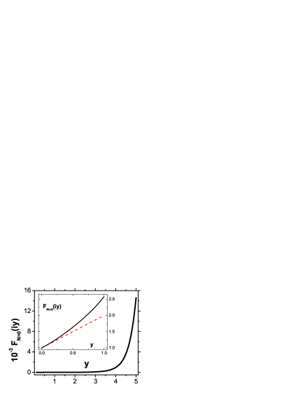
Figure 3: The function $F_{N=0}(iy)$. Dashed line represents small $y$ asymptotics (see text).

III.2 Fermionic propagator at $N=0$

In the limit $N=0$, the curvature of the Fermi surface scales out and the original 2D problem maps onto an effective 1D theory of electrons with retarded interaction (Refs. Lidsky, ; AIM, ). This allows one to compute fermion propagator by using 1D bosonization technique. The result for $G({\bf k},\omega_{m})$ can again be cast into the form of Eq. (1), but now Lidsky ; AIM

$$F_{N=0}(x)=\frac{3}{2}\exp\left\{(-1)^{5/4}\Gamma^{3/2}(5/3)x^{3/2}\right\}\quad\qquad\qquad$$

$$\qquad\qquad-\frac{3\sqrt{3}i}{4\pi}\int_{0}^{\infty}dy\;\frac{\exp\left\{i(\Gamma(5/3)xy)^{3/2}\right\}}{y^{2}+iy-1}.$$ (11)

The analysis of $F_{N=0}(x)$ is presented in Appendix A. The key point is that $F_{N=0}(x)$ is a regular function in any finite region in the upper half-plane, and, in particular, along imaginary $x=iy,y>0$, where there was a pole at large $N$. At small $x$, $F_{N=0}(x)$ expands in regular powers of $x$:

$$F_{N=0}(x=iy)=1+y+\frac{27\sqrt{3}}{16\pi}\;\Gamma^{3}(5/3)\;y^{2}+O(y^{3}).$$ (12)

At large $x$, $F_{N=0}(x=iy)$ grows exponentially with $y$, but still remains finite for all finite $y$. We plot $F_{N=0}(iy)$ in Fig. 3.

III.3 Nonanalytic terms in the self-energy

Our key interest is how the pole disappears between $N=0$ and $N>>1$. One possibility might have been that the pole drifts to higher $x$ with decreasing $N$, and disappears at $x=i\infty$ at $N=0$. That would be consistent with the divergence of $F_{N=0}(iy)$ at $y=\infty$. However, the expansion in $1/N$ at large $N$ shows that the pole actually drifts to smaller $x=iy$ with decreasing $N$. Another possibility would be a behavior in which the residue $Z_{N}$ of the pole gradually disappears at $N\rightarrow 0$, i.e., regular corrections to $Z_{N}$ (the ones which are of order $\ln^{2}N/N^{2}$ at large $N$) make $Z_{0}=0$. We, however, didn’t find a self-consistent solution for $Z_{N}$ and $D_{N}$ at small $N$ (this search required some computational efforts).

Below we assume that regular corrections to fermionic propagator leave $Z_{N}$ and $D_{N}$ finite at $N\rightarrow 0$, and the pole is destroyed by “universal” non-perturbative terms in the loop expansion of the self-energy near the mass shell. These terms appear at every order in the loop expansion, are non-analytic, and come from fermions with the lowest energies. We first identify these terms at $N=0$, and then show how they get modified at finite $N$.

III.3.1 N=0

The two-loop diagram is presented in Fig. 2 contains momentum and frequency integrals. At $N=0$, the curvature term that couples the two disappears (see Eq. B.1). The momentum and frequency integration in the self-energy then factorize, and the momentum integrals are straightforwardly evaluated leaving only non-trivial frequency integrals. The two-loop self-energy becomes

$$\Sigma_{2}(k,\omega_{m}) = i\omega_{m}^{2/3}\omega_{0}^{1/3}\left(\frac{\sqrt{3}}{2\pi}\right)^{2}\left(\frac{4\pi}{3\sqrt{3}}\right)^{2}\int_{0}^{1}\frac{d\Omega_{1}}{\Omega_{1}^{1/3}}\int_{1-\Omega_{1}}^{1}\frac{d\Omega_{2}}{\Omega_{2}^{1/3}}$$ (13)

$$\times \frac{1}{\Delta+\left[(1-\Omega_{1})^{2/3}+(1-\Omega_{2})^{2/3}+(\Omega_{1}+\Omega_{2}-1)^{2/3}-1\right]},$$

where $\Omega_{1}$ and $\Omega_{2}$ are two internal frequencies normalized by $\omega_{m}$, and, we remind, $\Delta=1+i\epsilon_{k}/(\omega^{2/3}_{m}\omega^{1/3}_{0})$. Note that the coupling ${\bar{g}}$ is fully absorbed into $\omega_{0}$, i.e., for a generic $\Delta=O(1)$, $\Sigma_{2}(k,\omega_{m})$ (as well as self-energies of higher-loop order) is of order $\omega^{2/3}\omega^{1/3}_{0}$, with a prefactor of order one.

Expanding Eq. (13) to first order in $\Delta$, we only obtain regular contributions to $Z_{0}$ and to $D_{0}$. These contributions are perturbative in the sense that typical internal $\Omega_{1,2}$ are of order one, much larger than $\Delta\ll 1$ over which one expands. However, this doesn’t go beyond first order – a formal expansion to order $\Delta^{2}$ yields a divergent prefactor. On more careful look, we found that the next term beyond $\Delta$ is actually $\Delta^{3/2}$. This term comes from the regions $\Omega_{1}<<1$, $1-\Omega_{2}=\Omega^{\prime}_{2}<<1$ and $\Omega_{2}<<1$, $1-\Omega_{1}=\Omega^{\prime}_{1}<<1$. The contributions from both regions are equal, and we only focus on the first one, for which the denominator in Eq. (13) becomes $\Delta+(\Omega^{\prime}_{2})^{2/3}+(\Omega_{1}-\Omega^{\prime}_{2})^{2/3}$. Rescaling $\Omega_{1}=\Delta^{3/2}x$, $\Omega^{\prime}_{2}=\Delta^{3/2}y$ and multiplying the self-energy by a factor of $2$ to account for the two regions, we re-write Eq. (13) as

$$\Sigma_{2}(k,\omega_{m}) = 8i\omega_{m}^{2/3}\omega_{0}^{1/3}\;\frac{\Delta^{3/2}}{9}$$

$$\times \!\!\int_{0}^{1/\Delta^{3/2}}\frac{dx}{x^{1/3}}\int_{0}^{x}\frac{dy}{1+y^{2/3}+(x-y)^{2/3}}.$$

The largest contribution to this integral is confined to the upper limit of the integration over $x$. This is a regular, perturbative term (internal frequency $(\Omega_{1})^{2/3}=\Delta x^{2/3}>>\Delta$). However, we also found a contribution which is confined to $x=O(1)$, i.e., to internal energies of order $\Delta^{3/2}$. For the integral in (III.3.1) this contribution can be easily singled out – it is given by

$$\Sigma_{2}(k,\omega_{m})\! = \!\Sigma_{2,reg}(k,\omega_{m})\qquad\qquad\quad+$$

$$+ 8i\omega_{m}^{2/3}\omega_{0}^{1/3}\frac{\Delta^{3/2}}{9}\int_{0}^{\infty}\frac{dx}{x^{1/3}}\int_{0}^{x}dy$$

$$\times \!\!\frac{1}{(1+y^{2/3}+(x-y)^{2/3})(y^{2/3}+(x-y)^{2/3})^{2}}.$$

Evaluating the integral numerically, we obtain

$$\Sigma_{2}(k,\omega_{m})=2.69\;i\omega_{m}^{2/3}\omega_{0}^{1/3}\Delta^{3/2}.$$ (16)

At the first glance, this term is smaller than $O(\Delta)$ and is irrelevant to the issue of pole disappearance. Let’s, however, continue our analysis and verify whether there are singular renormalizations of $\Sigma_{2}(k,\omega_{m})$ from three-loop and higher-order diagrams. We found that such renormalizations do exist and come from vertex corrections. In particular, for the universal contribution to $\Sigma_{2}$ from $\Omega_{1}<<1$, $1-\Omega_{2}=\Omega^{\prime}_{2}<<1$, singular renormalization comes from corrections to the two spin-boson vertices which involve bosonic propagator with the frequency $\Omega_{2}$. Each vertex correction contains a block made out of two extra Green’s functions and one interaction line. We verified that the corrections to the two vertices involving the propagator with $\Omega_{2}$ are the same, and each yields, after integrating over internal $\epsilon_{k}$

$$\frac{{\bar{g}}}{(2\pi)^{2}v_{\text{\tiny{F}}}}\int_{\omega\Omega_{1}}^{\omega}\frac{d\Omega}{\Sigma_{1}(\Omega)}\int\frac{dqq}{q^{3}+\gamma\Omega}=$$

$$\frac{2}{3}\int_{\Omega_{1}}^{1}\frac{dz}{z}=\frac{2}{3}\ln{\frac{1}{\Omega_{1}}}.$$ (17)

We see that vertex correction is logarithmic and large, if $\Omega_{1}\ll 1$. Typical $\Omega_{1}$ for the universal term in $\Sigma_{2}$ are of order $\Delta^{3/2}$, hence the leading vertex correction is $\ln\bigl{(}1/\Delta\bigr{)}$. Observe that the prefactor is just a number – the coupling ${\bar{g}}$ is canceled out by $(\gamma\omega_{0})^{1/3}\propto{\bar{g}}$. Evaluating higher-order corrections in the leading logarithmical approximation (in which we keep only the highest power of the logarithm at any order), we find that the full vertex $\Gamma$ becomes (see Fig. 2c)

$$\Gamma = 1+\ln\frac{1}{\Delta}+\frac{1}{2}\left(\ln\frac{1}{\Delta}\right)^{2}+\frac{1}{6}\left(\ln\frac{1}{\Delta}\right)^{3}+...$$ (18)

$$=e^{\ln\frac{1}{\Delta}}=\frac{1}{\Delta}.$$

This $\Gamma$ is the solution of the differential RG equation

$$\frac{d\Gamma}{dL}=\Gamma,\;\;L=\ln{\frac{1}{\Delta}}.$$ (19)

The implication is that the vertex correction can be treated within RG technique, i.e., that the system is renormalizable.

Eq. (18) is not exact, however, as there exist extra terms of order $\ln\bigl{(}1/\Delta\bigr{)}$ from second-order and higher-order vertex corrections. Such terms come with prefactors $O(1)$, and modify the exponent in (18) to

$$\Gamma\propto\frac{1}{\Delta^{a}},$$ (20)

where $a=O(1)$. Because the exponent $a$ has contributions from all orders, we cannot compute it explicitly within the loop expansion, nor verify explicitly that logarithmic series still exponentiate beyond the leading logarithmic approximation (i.e., that RG procedure leading to (20) is still valid). At the same time, the situation here is not different from a variety of other problems where RG treatment has been adopted based on the leading logarithmic series, AIM ; acs ; artem and we assume that Eq. (20) is valid without further reasoning.

Combining Eq. (20) with Eq. (16), we find that the universal part of the self-energy, dressed by logarithmic vertex renormalizations, behaves near the mass shell as

$$\Sigma_{univ}\sim i\omega_{m}^{2/3}\omega_{0}^{1/3}\Delta^{3/2-2a}.$$ (21)

To agree with the bosonization formula, we have to set $a=3/4$, then $\Sigma_{univ}$ becomes $\Delta$-independent, and the full Green’s function behaves near the former mass shell as $G^{-1}(k,\omega_{m})=i\omega^{2/3}_{m}\omega^{1/3}_{0}\left(A+B\Delta+...\right)$ where $A$ and $B$ are constants.

We now re-evaluate universal terms at $N\neq 0$ and see how the universal self-energy gets modified at a finite $N$.

III.3.2 Finite $N$

At a finite $N$, momentum and frequency integrals do not decouple, and the computations become more involved. Still, the two momentum integrals can be evaluated exactly, at any $N$, so the remaining task is to properly estimate the frequency integrals. As at $N=0$, we expand in $\Delta$ and verify whether or not this expansion contains the non-perturbative, universal term. We find that such term is again present, but at a finite $N$ and $\Delta<N^{2}$, scales as $\Delta^{5/2}$ rather than $\Delta^{3/2}$. This term comes from the same range of internal frequencies as at $N=0$ – one of the internal frequencies is small, another is close to external $\omega$. Using the same notations as at $N=0$, we obtain for the contribution from such region, with logarithmic accuracy

$$\Sigma_{2}(k,\omega_{m})=i\omega_{m}^{2/3}\omega_{0}^{1/3}\frac{\Delta^{5/2}}{4\pi^{2}N^{2}}$$

$$\times \!\int_{0}^{1/\Delta^{3/2}}\!\frac{dx}{x}\int_{0}^{x}dy\left(1+y^{2/3}+(x-y)^{2/3}\right)$$

$$\times \!\left[\ln\left(\frac{N}{\sqrt{\Delta}}\right)+\ln\left(\frac{x^{1/3}}{1+y^{2/3}+(x-y)^{2/3}}\right)\right]^{2}.$$

The universal term (the one which does not depend on the upper limit of integration) comes from the cross-product of the two logarithms, and the universal part of the two-loop self-energy is

$$\Sigma_{2}(k,\omega_{m})=i\omega_{m}^{2/3}\omega_{0}^{1/3}\Delta^{5/2}\frac{J}{8\pi^{2}N^{2}}~{}\ln{\frac{N^{2}}{\Delta}}.\;\;\;\;\;\;\;$$ (23)

The prefactor $J$ is given by

$$J=-\int_{0}^{\infty}dx\int_{0}^{1}dz\psi(x,z),$$ (24)

where

$$\psi(x,z)\!\! = \!\!\ln\left(1+\frac{1}{x^{2/3}f_{z}}\right)-\frac{1}{x^{2/3}f_{z}}+x^{2/3}f_{z}$$

$$\times \!\!\left[\ln\left(1+\frac{1}{x^{2/3}f_{z}}\right)-\frac{1}{x^{2/3}f_{z}}+\frac{1}{2}\left(\frac{1}{x^{2/3}f_{z}}\right)^{2}\right],$$

and $f_{z}=z^{1/3}+(1-z)^{1/3}$. Evaluating the integral, we obtain $J\approx 0.96$.

The next step is to include vertex renormalizations from higher-order diagrams, i.e., renormalize the universal part of $\Sigma_{2}$ in (23) into $\Sigma_{2,univ}=\Sigma_{2}*\Gamma^{2}$. We found that multi-loop contributions to $\Gamma$ are again logarithmic, but now the lower limit of the logarithm is set by the largest of $\Delta$ and $N^{2}$. The full result is then $\Gamma\propto 1/\Delta^{3/4}$ for $\Delta\gg N^{2}$ and $\Gamma\propto 1/N^{3/2}$ for $\Delta<<N^{2}$. Combining this with (23), we obtain

$$\Sigma_{univ}\sim i\omega_{m}^{2/3}\omega_{0}^{1/3}g\left(\frac{\Delta}{N^{2}}\right),$$ (26)

where $g(y<<1)\propto y^{5/2}$ and $g(y>>1)={\text{c}onst}$. We neglected $\ln{\Delta/N^{2}}$ term because $\Gamma$ is only known to the accuracy that neglects possible additional logarithmical factors.

Substituting the full $\Sigma_{univ}$ into the Green’s function, we reproduce Eq. (3):

$$G(k,\omega_{m})=-\frac{1}{\epsilon_{k}}F_{N\rightarrow 0}\left(\Delta\right);$$

$$F_{N\rightarrow 0}\left(\Delta\right)=\frac{1}{-\Delta+g\left(\Delta/N^{2}\right)}.$$ (27)

We see that the pole survives, at the smallest $\Delta$ for any nonzero $N$ and, moreover, its residue remains $Z_{N}=O(1)$. However, at distances from the pole larger than $N^{2}$, the system evolves, and its behavior becomes essentially the same as at $N=0$.

IV Half-filled Landau level

In this section we study different example of a non-Fermi liquid behavior - 2D fermions at half-filled Landau level with unscreen Coulomb interaction. Jain ; Halperin ; AIM The effective low-energy theory is described by Eq. (4) with massless bosonic propagator

$$\chi(q,\omega)=\frac{\chi_{0}}{muq+\gamma\;|\omega/q|}.$$ (28)

Here $u$ is the effective velocity [$u=e^{2}/(8\pi{\hat{\epsilon}})$ with ${\hat{\epsilon}}$ the dielectric constant of a host semiconductor], and $\gamma={\bar{g}}k_{\text{\tiny{F}}}/(\pi v^{2}_{\text{\tiny{F}}})$ is the same as in the $\omega^{2/3}$ problem.

We start by presenting the results for the limiting cases $N\rightarrow\infty$ and $N=0$. Large $N$ limit is studied in $1/N$ expansion while $N=0$ is obtained via 1D bosonization. We then discuss our results for the universal terms in the loop expansion near the mass-shell.

IV.1 Fermionic propagator at $N>>1$

The one-loop self-energy has been calculated in Ref. AIM, . It has the form

$$\Sigma_{1}(\omega_{m})=i\lambda\;\omega_{m}\ln\biggl{(}\frac{\epsilon_{0}}{|\omega_{m}|}\biggr{)},$$ (29)

where $\lambda=\bar{g}/\left(4\pi^{2}uk_{\text{\tiny{F}}}\right)$ is a dimensionless coupling and $\epsilon_{0}$ is an energy scale defined by $\epsilon_{0}=(2\pi/N)\left(E_{\text{\tiny{F}}}/\bar{g}\right)uk_{\text{\tiny{F}}}$. The momentum dependent part of $\Sigma$ is regular and we neglect it. The $\omega\log\omega$ form of the self-energy Eq. (29) implies that the system exhibits a marginal non-Fermi liquid behavior, however the Fermi surface remains well defined.

As in the previous case, higher order self-energy diagrams are parametrically small in $(\ln N/N)^{2}$. Near the mass-shell $\tilde{\Delta}=0$, where

$$\tilde{\Delta}=1+\frac{i\epsilon_{k}}{\lambda\omega_{m}\ln\left(\epsilon_{0}/\omega_{m}\right)},$$ (30)

we found at two-loop order (see Appendix C) that $\Sigma_{2}(k,\omega_{m})$ is linear in $\tilde{\Delta}$

$$\Sigma_{2}(k,\omega_{m})=i\lambda\omega_{m}\ln\left(\epsilon_{0}/\omega_{m}\right)\frac{\tilde{\Delta}}{24}\left(\frac{\ln N}{N}\right)^{2}.$$ (31)

We see that, as for the $\omega^{2/3}$ problem, multi-loop self-energy terms acquire extra powers of $(\ln N/N)^{2}$. Substituting one- and two-loop self energies into the Green’s function and rewriting it as in Eqs. (1), (9), we obtain $G({\bf k},\omega_{m})=-\left(1/\epsilon_{k}\right)\tilde{F}_{N}(-y)$, where $y=\left(\Sigma_{1}/i\epsilon_{k}\right)$, and $\tilde{F}_{N\rightarrow\infty}(y)$ is again given by Eq. (9), but now

$$Z_{N}=1-\frac{1}{24}\;\left(\frac{\ln N}{N}\right)^{2},~{}~{}D_{N}=1.$$ (32)

We see that $1/N$ corrections for the Landau level case are qualitatively similar to the case of a nematic QCP – in both cases, the pole in $G({\bf k},\omega_{m})$ viewed as a function of $\epsilon_{k}$ survives, but acquires a residue $Z_{N}<1$.

In real space, we have (see Appendix C.1)

$$G({\bf r})=G_{0}({\bf r})\left[\frac{1}{\ln(r/r_{0})}\right],v_{F}t<r\ln{r/r_{0}},$$

$$G({\bf r},t)\approx G_{0}({\bf r},t),\;\;\;\;v_{\text{\tiny{F}}}t>r\ln(r/r_{0}),$$ (33)

where $G_{0}({\bf r},t)\propto(r+v_{\text{\tiny{F}}}t)^{-1}\sqrt{k_{\text{\tiny{F}}}/r}$ is a propagator of a free fermion, and $r_{0}=v_{\text{\tiny{F}}}/\epsilon_{0}$.

IV.2 Low-energy effective theory for $N=0$: Fermionic propagator

As in the previous case, at $N=0$ the curvature of the Fermi surface becomes unimportant, the motion of fermions becomes essentially one-dimensional, and the fermionic propagator can be obtained by mapping the original 2D problem to an effective 1D theory. Lidsky ; AIM For a half-filled Landau level the effective action has the form

$${\mathcal{S}}=\int\!d\Omega dk\qquad\qquad\qquad\qquad\qquad\qquad\qquad\qquad\;$$ (34)

$$\times\Bigl{[}\bar{\psi}_{-\Omega,-k}^{R,a}\bigl{(}i\Omega-v_{\text{\tiny{F}}}k\bigr{)}\psi_{\Omega,k}^{R,a}+\bar{\psi}_{-\Omega,-k}^{L,a}\bigl{(}i\Omega+v_{\text{\tiny{F}}}k\bigr{)}\psi_{\Omega,k}^{L,a}$$

$$+\left(4\pi^{2}\lambda v_{\text{\tiny{F}}}\right)\ln\Omega\;|\rho^{R}_{\Omega,k}-\rho^{L}_{\Omega,k}|^{2}\Bigr{]},$$

where $\rho_{\omega,k}=\bar{\psi}_{\omega,k}^{a}\psi_{\omega,k}^{a}$ is the density operator, and the replica index $a$ has $s$ values. As usual, we take the limit $s\rightarrow 0$ in order to avoid generating fermionic loops in perturbation theory.

We solve the model Eq. (34) by 1D bosonization. Following the standard steps we find that

$$G^{1D}(r,\tau)=\frac{i}{2\pi(r-iv_{\text{\tiny{F}}}\tau)}\exp\left[-\lambda\;\frac{r\ln|r-iv_{\text{\tiny{F}}}\tau|}{(r-iv_{\text{\tiny{F}}}\tau)}\right],$$

where $\tau$ is Matsubara time. A Fourier transform of Eq. (IV.2) yields a simple scaling form for $G({\bf k},\omega_{m})$:

$$G({\bf k},\omega_{m})\! = \!-\frac{1}{\epsilon_{k}}\tilde{F}_{N=0}\left[\frac{-\lambda\omega_{m}\ln\left({\epsilon_{0}}/{|\omega_{m}|}\right)}{\epsilon_{k}}\right],$$

$$\tilde{F}_{N=0}(x)\! = \!e^{-ix}.$$ (36)

We verified that the loop expansion reproduces the small $x$ expansion of $\tilde{F}_{N=0}(x)$. Obviously, $\tilde{F}_{N=0}(x)$ has no poles along $x=iy$ where $\tilde{F}_{N=0}(iy)=e^{y}$. We verified that the singularity at $y\rightarrow\infty$ is responsible for the exponential behavior of $G({\bf r},t)$ in (IV.2).

IV.3 Nonanalytic terms in the self-energy

IV.3.1 $N=0$

The relevant two-loop self-energy is again given by the diagram in Fig. 2a. We compute it in Appendix C for arbitrary $N$. As in the previous case, consider first $N=0$. We have

$$\Sigma_{2}(k,\omega_{m})=i\lambda\;\omega_{m}\int_{0}^{1}d\Omega_{1}\int_{1-\Omega_{1}}^{1}d\Omega_{2}$$ (37)

$$\frac{\ln\left[\epsilon_{0}/(\omega_{m}\Omega_{1})\right]\;\ln\left[\epsilon_{0}/(\omega_{m}\Omega_{2})\right]}{\tilde{\Delta}\ln\left(\epsilon_{0}/\omega_{m}\right)+\left\{(1-\Omega_{1})\ln\left[\frac{1}{1-\Omega_{1}}\right]+(1-\Omega_{2})\ln\left[\frac{1}{1-\Omega_{2}}\right]+(\Omega_{1}+\Omega_{2}-1)\ln\left[\frac{1}{\Omega_{1}+\Omega_{2}-1}\right]\right\}},$$

where $\Omega_{1}$ and $\Omega_{2}$ are the two internal energies normalized by $\omega_{m}$. In the previous case, $\Sigma_{2}$ was regular to first order in $\Delta$. This time, expanding Eq. (37) to first order in $\tilde{\Delta}$ we found that the prefactor diverges logarithmically. This suggests that the term next to the constant is already nonanalytic. We explicitly verified that the nonanalyticity emerges in Eq. (37) from the regions $\Omega_{1}\ll 1$, $\Omega_{2}\sim 1$ and $\Omega_{2}\ll 1,\Omega_{1}\sim 1$. Within the logarithmic accuracy, the nonanalytic contribution to $\Sigma_{2}$ can then be cast into the form

$$\Sigma_{2}(k,\omega_{m})=-2i\lambda\omega_{m}\;\tilde{\Delta}\;\ln^{2}\left(\epsilon_{0}/\omega_{m}\right)$$

$$\times\int_{\frac{{\tilde{\Delta}}\ln{\left(\epsilon_{0}/\omega_{m}\right)}}{|\ln{\tilde{\Delta}}|}}^{1}\frac{d\Omega_{1}}{\Omega_{1}\ln{1/\Omega_{1}}}$$

$$=-2i\lambda\;\omega_{m}{\tilde{\Delta}}\;\ln^{2}\left(\epsilon_{0}/\omega_{m}\right)\;\ln\ln\left(\frac{1}{\tilde{\Delta}}\right).$$ (38)

As before, higher-order diagrams modify Eq. (IV.3.1) by adding vertex corrections. A building block for a vertex correction is again the product of two fermionic Green’s functions and one interaction line. Evaluating this block we find that vertex corrections are again logarithmical. Using further the fact that typical dimensionless external energy for the correction to the vertex involving a boson with $\Omega_{2}$ is of order $\Omega_{1}$, we obtain the renormalized vertex ${\tilde{\Gamma}}$ in the form

$${\tilde{\Gamma}}=1+\ln\left(1/\Omega_{1}\right).$$ (39)

Evaluating further higher-order vertex corrections, we obtain in the leading logarithmical approximation

$${\tilde{\Gamma}} = 1+\ln{\frac{1}{\Omega_{1}}}+\frac{1}{2}\left(\ln{\frac{1}{\Omega_{1}}}\right)^{2}+\ldots$$ (40)

$$=e^{\ln{1/\Omega_{1}}}=\frac{1}{\Omega_{1}}.$$

As in the previous case, the exponent is modified by higher-order corrections to

$${\tilde{\Gamma}}\sim\left(\frac{1}{\Omega_{1}}\right)^{b}.$$ (41)

A simple experimentation shows that the full universal self-energy $\Sigma_{univ}=\Sigma_{2}{\tilde{\Gamma}}^{2}$ agrees with bosonization if we set $b=1/2$. Indeed, in this case, we have, combining Eqs. (41) and (IV.3.1)

$$\Sigma_{univ}=-ic\lambda\;\omega_{m}{\tilde{\Delta}}\ln^{2}\left(\epsilon_{0}/\omega_{m}\right)\times$$ (42)

$$\int_{\frac{{\tilde{\Delta}}\ln{\left(\epsilon_{0}/\omega_{m}\right)}}{|\ln{\tilde{\Delta}}|}}^{1}\frac{d\Omega_{1}}{\Omega^{1+2b}_{1}\;[\ln{1/\Omega_{1}}]}=-ic\lambda\omega_{m}\ln\left(\epsilon_{0}/\omega_{m}\right),$$

where $c=O(1)$. We see that the fully renormalized $\Sigma_{univ}$ tends to a finite value on the mass shell, i.e.,

$$G^{-1}\bigl{(}\tilde{\Delta}\bigr{)}=i\lambda\omega_{m}\ln\left(\epsilon_{0}/\omega_{m}\right)\left[{\tilde{\Delta}}+c\right].$$ (43)

This behavior is consistent with the bosonization formula, Eq. (IV.2) which yields $G^{-1}\propto(1+{\tilde{\Delta}})$ near the mass shell. The computation of the constant $c$ is beyond the scope of our analysis.

IV.3.2 Finite $N$

We now check how the expression for the self-energy is modified at finite $N$. Just like at $N=0$, we expand the two-loop self-energy in powers of $\tilde{\Delta}$ and extract the universal term in the prefactor. We find that, to logarithmical accuracy, the linear in ${\tilde{\Delta}}$ term is already universal, like at $N=0$, and the only difference between $N=0$ and $N>0$ cases is in lower limit of the frequency integration over $\Omega_{1}$: at a finite $N$, instead of ${\tilde{\Delta}}$, as in (IV.3.1), we now have $N^{2}$. Accordingly, instead of ((IV.3.1), we now have

$$\Sigma_{2}(k,\omega_{m}) = -i\lambda\;\omega_{m}\;\ln^{2}\left(\epsilon_{0}/\omega_{m}\right)\;\tilde{\Delta}\ln\ln(1/N).$$

As the next step, we include vertex corrections. They are still logarithmical and exponentiate, as in (41), but now typical $\Omega_{1}$ are of order $N^{2}$, hence

$$\Sigma_{univ}\propto-i\lambda\;\omega_{m}\ln^{2}\left(\epsilon_{0}/\omega_{m}\right)\;\frac{\tilde{\Delta}}{N^{2}}.$$ (45)

We neglected $\ln|\ln N|$ factor as the renormalized vertex is only known to this accuracy. We see that $\Sigma_{univ}$ is still linear in $\Delta$, i.e., the pole in the Green’s function survives in the range of order $N^{2}$. This is similar to $\omega^{2/3}$ case. Unlike that case, however, the residue of the pole scales as $N^{2}$ and vanishes when $N=0$. Substituting $\Sigma_{univ}$ into the Green’s function and rewriting the result in terms of $\tilde{F}_{N}$, as in (IV.2), we obtain near the mass shell

$$G({\bf k},\omega_{m})\!=\!-\frac{1}{\epsilon_{k}}\tilde{F}_{N\rightarrow 0}\left({\tilde{\Delta}}\right),$$

$$\tilde{F}_{N\rightarrow 0}\left({\tilde{\Delta}}\right)={\tilde{F}}\left(\frac{\tilde{\Delta}}{N^{2}}\right),$$ (46)

where ${\tilde{F}}(y\ll 1)\propto y,\>{\tilde{F}}(y\gg 1)={\text{c}onst}$.

The difference in $Z_{N}$ between the QCP and the Landau level cases is due to the fact that in the case of a Landau level the universal self-energy already emerges in the loop expansion already at order ${\tilde{\Delta}}$ while at a nematic QCP it appears at order $\Delta^{3/2}$. There may also be additional differences between the scaling functions $F_{N\rightarrow 0}$ and ${\tilde{F}}_{N\rightarrow 0}$ due to extra logarithmic or doubly logarithmic factors, but, as we said, these factors are beyond the slope of our paper.

V conclusions

In this paper we considered two examples of 2D fermions coupled to critical overdamped bosonic fields. One describes a nematic and an Ising ferromagnetic quantum critical points, other describes a half-filled Landau level. For both cases, the low-energy physics is governed by the interaction between fermions and collective neutral excitations with the static propagator $\chi(q)=\chi_{0}/q^{1+x}$. For a nematic and ferromagnetic QCP $x=1$, for a half-filled Landau level with unscreened Coulomb interaction, $x=0$. In both cases, quantum fluctuations destroy a coherent Fermi liquid behavior down to the lowest energies, but leave the Fermi surface intact. The issue we addressed is what is the form of the fermionic propagaror, and whether it has a pole as a function of the dispersion $\epsilon_{k}$.

The low energy properties of these systems can be studied in a controllable way by extending the theory to $N>>1$ fermionic flavors and assuming that the interaction with neutral excitations conserves the flavor. At large $N$, self-energy is perturbative in $1/N$, and the pole in the Green’s function survives despite that $\Sigma(k_{\text{\tiny{F}}},\omega)\propto\omega^{2/3}$ for $x=1$ and $\Sigma(k_{\text{\tiny{F}}},\omega)\propto\omega\log\omega$ for $x=0$. $1/N$ corrections only affect the residue of the pole $Z_{N}$ and make $Z_{N}<1$. Existence of the pole implies that the propagator in real space/time is long ranged and decays by a power-law, e.g., as $G(r\gg v_{\text{\tiny{F}}}t)\propto 1/r^{2}$ and $G(r\ll v_{\text{\tiny{F}}}t)\propto 1/t\sqrt{r}$ for $x=1$. The other limit $N=0$, has been solved using 1D bosonization, and the result is that for both $x=1$ and $x=0$, fermionic propagator does not have a pole, and the propagator $G(r,t)$ is short-ranged.

The issue we addressed is at what $N$ the pole disappears. This is essential as the physical case $N=1$ is “in between” the two limits. We performed the loop expansion for the self-energy both at $N=0$ and at a finite but small $N$. At $N=0$, we identified universal, non-analytic contributions to $\Sigma$ which destroy the pole and make fermionic propagator regular near the former mass shell. At small but nonzero $N$, we found that singular, universal terms in the self-energy still exist, but they do not destroy the pole in the range of order $N^{2}$ around the mass shell. At larger deviations from the mass shell, fermionic propagator recovers the same regular form as at $N=0$. For a nematic QCP, the residue of the pole $Z_{N}$ remains $O(1)$ in this range, while for the case of a half-filled Landau level, the residue of the pole scales as $Z_{N}\propto N^{2}$.

The result that the pole in $G(k,\omega_{m})$ exists for any $N>0$ and only vanishes at $N=0$ agrees with the conjecture by Altshuler et al AIM . The key result of our work is the identification of peculiar, universal terms in the loop expansion of the self-energy, which are responsible for the destruction of the pole at $N=0$. At $N>0$, these terms get modified – they do not destroy the pole but reduce the width where the pole exists.

VI acknowledgement

We acknowledge with thanks useful conversations with E. Fradkin, D. Khveshchenko, Y. B. Kim, M. Lawler, W. Metzner, and T. Senthil. The work was supported by NSF-DMR 0604406 (A. V. C) and by Herb foundation (T. A. S).

Appendix A Analysis of the fermion propagator at a QCP at $N\rightarrow\infty$ and $N=0$

In this Appendix we analyze the behavior of the fermion propagator

$$G({\bf r},\tau)=\int_{-\infty}^{\infty}\frac{d\omega_{m}}{2\pi}\int\frac{d{\bf k}}{(2\pi)^{2}}\;e^{i{\bf k}{\bf r}-i\omega_{m}\tau}G({\bf k},\omega_{m}),$$ (47)

at a nematic QCP at $N>>1$ and $N=0$. The goal of this analysis is to demonstrate that the form of long-distance behavior of $G({\bf r},\tau)$, where $\tau$ is the Matsubara time, is qualitatively different depending on whether or not $G({\bf k},\omega_{m})$ has a pole as a function of $\epsilon_{k}$.

We use the Matsubara frequency form of $G(\epsilon_{k},\omega_{m})=-(1/\epsilon_{k})F_{N}\left(-\omega_{m}^{2/3}\omega^{1/3}_{0}/\epsilon_{k}\right)$. Introducing new variables, $x=-(\omega_{m}^{2/3}\omega^{1/3}_{0})/\epsilon_{k}$, $y=(\epsilon_{k}r/v_{\text{\tiny{F}}})$ and $\alpha=\left(v_{\text{\tiny{F}}}^{3/2}\tau/\omega_{0}^{1/2}r^{3/2}\right)$ we re-write Eq. (47) as

$$G({\bf r},\tau)\!\! = \!\!\frac{3}{2r^{2}}\left(\frac{1}{\pi^{3/2}}\right)\sqrt{\frac{E_{\text{\tiny{F}}}}{\omega_{0}}}\int_{-\infty}^{\infty}dx|x|^{1/2}\!\int_{-\infty}^{\infty}\!dy|y|^{1/2}$$

$$\!\times \!\cos\left(k_{\text{\tiny{F}}}r+y-\frac{\pi}{4}\right)F_{N}(x)e^{-i(-1)^{3/2}x^{3/2}y^{3/2}\alpha}.$$

A.1 Limit $N\rightarrow\infty$

In this limit $F_{N=\infty}(x)=1/(1+ix)$. Substituting this into Eq. (A), we obtain

$$G({\bf r},\tau) = \frac{1}{r^{2}}\left(\frac{3}{2\pi^{3/2}}\right)\sqrt{\frac{E_{\text{\tiny{F}}}}{\omega_{0}}}\int_{-\infty}^{\infty}dx\int_{-\infty}^{\infty}dy\;|xy|^{1/2}$$ (49)

$$\times \frac{e^{-i(-1)^{3/2}x^{3/2}y^{3/2}\alpha}}{1+ix}\cos\left(k_{\text{\tiny{F}}}r+y-\frac{\pi}{4}\right).$$

We now show that the pole at $x=-i$ determines long-distance behavior of $G({\bf r},t)$. For definiteness, we focus on the case $\alpha<<1$, i.e., $v_{\text{\tiny{F}}}^{3/2}\tau<<\omega_{0}^{1/2}r^{3/2}$. In this limit, the exponential factor in (49) can be set to unity and the integrals decouple. Integration over $y$ is straightforward and yields

$$\lim_{\lambda\rightarrow 0^{+}}\int_{-\infty}^{\infty}dy|y|^{1/2}\cos\left(k_{\text{\tiny{F}}}r+y-\frac{\pi}{4}\right)e^{-\lambda|y|}$$

$$=-\sqrt{\frac{\pi}{2}}\cos\left(k_{\text{\tiny{F}}}r-\frac{\pi}{4}\right).$$ (50)

We added the factor $e^{-\lambda|y|}$ for regularization. The subsequent integration over $x$ is also straightforward.

$$\int_{-\infty}^{\infty}dx\frac{|x|^{1/2}}{1+ix}=2\int_{0}^{\infty}dx\frac{x^{1/2}}{1+x^{2}}=\sqrt{2}\pi.$$ (51)

We also evaluated the integral in Eq. (51) by extending the integration into the complex plane of $x$ and found that the result comes from the pole at $x=i$, the branch cut contribution in (51) is cancelled out. Substituting Eqs. (A.1) and (51) into Eq. (49) we find that the fermion propagator $G({\bf r},\tau)\propto 1/r^{2}$ at $v_{F}\tau\ll r^{3/2}/r_{0}^{1/2}$, where $r_{0}=v_{F}/\omega_{0}$. We emphasize again that the power-law decay is the consequence of the pole in $G({\bf k},\omega_{m})$.

For completeness, we also present the result for $G({\bf r},\tau)$ for $\alpha\gg 1$ . In this case we obtained

$$G({\bf r},\tau)=\frac{1}{r^{2}}\left(\frac{3}{\sqrt{2\pi}}\right)\sqrt{\frac{E_{\text{\tiny{F}}}}{\omega_{0}}}\;{\cal K}(\alpha),$$ (52)

where

$${\cal K}(\alpha)\text{\Large{$|$}}_{\alpha\rightarrow\infty}=\frac{2\sqrt{2}}{3\alpha}\cos\left(k_{\text{\tiny{F}}}r-\frac{\pi}{4}\right).$$ (53)

Using $\alpha\propto\tau/r^{3/2}$ we find that in this limit the real space/time Green’s function behaves as $G({\bf r},\tau)\propto 1/\left(\sqrt{r}v_{\text{\tiny{F}}}\tau\right)$. Combining the two results, we have

$$G({\bf r},\tau)\text{\Large{$|$}}_{N\rightarrow\infty}\propto\left\{\begin{array}[]{c}\frac{1}{r^{2}},\;\;\;v_{\text{\tiny{F}}}\tau\ll r^{3/2}/r_{0}^{1/2}\\ \frac{k_{\text{\tiny{F}}}}{v_{\text{\tiny{F}}}\tau}\sqrt{\frac{r_{0}}{r}},\;\;\;v_{\text{\tiny{F}}}\tau\gg r^{3/2}/r_{0}^{1/2}\\ \end{array}\right.,$$ (56)

or, in terms of the free-fermion propagator $G_{0}({\bf r},\tau)$,

$$G({\bf r},\tau)\text{\Large{$|$}}_{N\rightarrow\infty}=\left\{\begin{array}[]{c}G_{0}({\bf r},\tau)\sqrt{r_{0}/r},\;\;\;v_{\text{\tiny{F}}}\tau\ll r^{3/2}/r_{0}^{1/2}\\ G_{0}({\bf r},\tau)\sqrt{k_{\text{\tiny{F}}}r_{0}},\;\;\;v_{\text{\tiny{F}}}\tau\gg r^{3/2}/r_{0}^{1/2}\\ \end{array}\right..$$

A.2 Limit $N=0$

The expression for $G(k,\omega_{m})$ in this case is given in Ref. AIM, , see Eq. (11). The function $F_{N=0}(x)$ in (11) can be represented as

$$F_{N=0}(x) = \cosh\left[e^{i\pi/4}\Gamma^{3/2}(5/3)x^{3/2}\right]-ix\;{\mathcal{F}}_{1}(x)$$ (59)

$$- x^{2}\frac{27\sqrt{3}}{16\pi}\Gamma^{3}(5/3)\;{\mathcal{F}}_{2}(x),$$

where ${\mathcal{F}}_{1}$ and ${\mathcal{F}}_{2}$ are expressed in terms of hypergeometric functions

$${\mathcal{F}}_{1}(x)=\text{\tiny{1}}\large{F}\text{\tiny{2}}\left[1;5/6,4/3;(1/4)i\Gamma^{3}(5/3)\;x^{3}\right],$$

$${\mathcal{F}}_{2}(x)=\text{\tiny{1}}\large{F}\text{\tiny{2}}\left[1;7/6,5/3;(1/4)i\Gamma^{3}(5/3)\;x^{3}\right].$$ (60)

At small arguments, ${\mathcal{F}}_{1}(x)$ and ${\mathcal{F}}_{2}(x)$ are expandable in $x$ AIM

$${\mathcal{F}}_{1}(x)\!=\!1+\frac{9}{40}i\left[\Gamma(5/3)x\right]^{3}-\frac{81}{6160}\left[\Gamma(5/3)x\right]^{6}+O\left[ix^{9}\right],$$

$${\mathcal{F}}_{2}(x)\!=\!1+\frac{9}{70}i\left[\Gamma(5/3)x\right]^{3}-\frac{81}{14560}\left[\Gamma(5/3)x\right]^{6}+O\left[ix^{9}\right].$$

By contrast, at large $|x|\gg 1$, $F_{N=0}(x)$ diverges as

$$F_{N=0}(x) = \frac{3}{2}\exp\left[-e^{i\pi/4}\Gamma^{3/2}(5/3)x^{3/2}\right]$$

$$+ \left[-\frac{3i\sqrt{3}}{4\pi x}-\frac{2}{9\Gamma^{3}(5/3)x^{2}}-O\left[1/x^{4}\right]\right].$$

Still, along $x=iy$ $F_{N=0}(iy)$ as a regular function of $y$ for all finite $y$, i.e., there is no pole. The plot of $F_{N=0}(iy)$ versus $y$ is presented in Fig. 3.

Below we show that the absence of the pole eliminates a power-law decay of $G(r,\tau)$, while the divergence of $F_{N=0}(x)$ at infinity gives rise to the exponential decay of the fermionic propagator.

The easiest way to evaluate the integral over $x$ in Eq. (A) with $F_{N=0}(x)$ given by Eq. (59) is to deform the integration contour into the complex plane. As for large $N$, the contribution from the branch cut is canceled out and in the absence of the pole $G(r,\tau)$ only comes from the integral over a semi-circle with infinite radius. Using parametrization

$$x^{3/2}=R^{3/2}\exp\left\{i\varphi\right\},\;\;\;\;\pi<\varphi<2\pi,$$ (63)

with $R\rightarrow\infty$, substituting into (A) the large-$x$ asymptote of $F_{N=0}$

$$F_{N=0}(x)=\frac{3}{2}\exp\left[-e^{i\pi/4+i\varphi}\Gamma^{3/2}(5/3)R^{3/2}\right],$$ (64)

and introducing $y_{1}=\alpha^{2/3}y$, we obtain

$$G({\bf r},\tau)=-\frac{1}{\alpha r^{2}}\left(\frac{3}{2\pi^{3/2}}\right)\sqrt{\frac{E_{\text{\tiny{F}}}}{\omega_{0}}}\int_{-\infty}^{\infty}dy_{1}|y_{1}|^{1/2}$$

$$\times\cos\left(k_{\text{\tiny{F}}}r+\left[y_{1}/\alpha^{2/3}\right]-\frac{\pi}{4}\right)\int_{\pi}^{2\pi}\!d\varphi\;iR^{3/2}e^{i\varphi}$$

$$\times\frac{3}{2}\exp\left\{R^{3/2}e^{i\varphi}\left[-iy_{1}^{3/2}-e^{i\pi/4}\Gamma^{3/2}(5/3)\right]\right\}.$$

Integrating over the angular variable $\varphi$ we obtain

$$R^{3/2}\int_{\pi}^{2\pi}d\left\{e^{i\varphi}\right\}\exp\Biggl{\{}R^{3/2}e^{i\varphi}\qquad\;\;$$

$$\qquad\times\left[-iy_{1}^{3/2}-e^{i\pi/4}\Gamma^{3/2}(5/3)\right]\Biggr{\}}$$

$$={2\pi}\;\delta\left[iy_{1}^{3/2}+e^{i\pi/4}\Gamma^{3/2}(5/3)\right],\quad$$ (66)

where $\delta(...)$ is the $\delta$-function. The integration over $y_{1}$ is then straightforward and yields

$$G({\bf r},\tau)=-\frac{1}{\alpha r^{2}}\left(\frac{3}{\pi^{1/2}}\right)\sqrt{\frac{E_{\text{\tiny{F}}}}{\omega_{0}}}\int_{-\infty}^{\infty}dy_{1}|y_{1}|^{1/2}\times$$

$$\cos\left(k_{\text{\tiny{F}}}r+\left[y_{1}/\alpha^{2/3}\right]-\frac{\pi}{4}\right)\delta\left[iy_{1}^{3/2}+e^{i\pi/4}\Gamma^{3/2}(5/3)\right]$$

$$\propto\frac{1}{\tau\sqrt{r}}\exp\left\{-\frac{\Gamma(5/3)}{(i)^{2/3}\alpha^{2/3}}\right\}.$$ (67)

Re-expressing $\alpha$ in terms of $r$ and $t$, we finally obtain

$$G({\bf r},\tau)\propto\frac{k_{\text{\tiny{F}}}}{v_{\text{\tiny{F}}}\tau}\sqrt{\frac{r_{0}}{r}}\exp\Biggl{(}-\frac{\Gamma(5/3)r}{r_{0}^{1/3}\bigl{[}iv_{\text{\tiny{F}}}\tau\bigr{]}^{2/3}}\Biggr{)}.$$ (68)

We see that $G(r,\tau)$ is now exponential. The full bosonization result contains $(iv_{\text{\tiny{F}}}\tau-r)$ instead of $iv_{\text{\tiny{F}}}\tau$ in denominator of (68) (see Ref. Lidsky, ). To reproduce it, we would need more complex form of $G(k,\omega_{m})$ than the one we borrowed from Ref. AIM, .

Appendix B Two-loop contribution to the self-energy at a QCP.

In this Appendix, we show the details of the calculations of the two-loop and three-loop self-energy diagrams.

B.1 Two-loop diagram

The diagram is presented in Fig. 2. In analytic form

$$\Sigma_{2}(k,\omega_{m}) = -g^{4}\int\frac{d\omega_{1}\;d{\bf q}_{1}}{(2\pi)^{3}}\int\frac{d\omega_{2}\;d{\bf q}_{2}}{(2\pi)^{3}}\;\chi({\bf q}_{1},\omega_{1})\chi({\bf q}_{2},\omega_{2})G({\bf k}+{\bf q}_{1},\omega_{m}-\omega_{1})$$

$$\times G({\bf k}+{\bf q}_{2},\omega_{m}-\omega_{2})G({\bf k}+{\bf q}_{1}+{\bf q}_{2},\omega_{m}-\omega_{1}-\omega_{2})$$

$$= \frac{\bar{g}^{2}}{(2\pi)^{6}}\int d\omega_{1}d{\bf q}_{1}\int d\omega_{2}d{\bf q}_{2}\frac{|q_{1}|}{\gamma|\omega_{1}|+|q_{1}|^{3}}\frac{|q_{2}|}{\gamma|\omega_{2}|+|q_{2}|^{3}}$$

$$\times \left[\frac{1}{\tilde{\Sigma}(\omega_{m}-\omega_{1})-v_{\text{\tiny{F}}}(k_{x}+q_{1x})-N(k_{y}+q_{1y})^{2}/2m}\right]\left[\frac{1}{\tilde{\Sigma}(\omega_{m}-\omega_{2})-v_{\text{\tiny{F}}}(k_{x}+q_{2x})-N(k_{y}+q_{2y})^{2}/2m}\right]$$

$$\times \left[\frac{1}{\tilde{\Sigma}(\omega_{m}-\omega_{1}-\omega_{2})-v_{\text{\tiny{F}}}(k_{x}+q_{1x}+q_{2x})-N(k_{y}+q_{1y}+q_{2y})^{2}/2m}\right].$$

Integrating over $q_{1x}$ and $q_{2x}$ and rescaling frequencies $\omega_{1}$, $\omega_{2}$ by $\omega_{m}$ and momenta $q_{1y},\;q_{2y}$ by $(\gamma\omega_{1,2})^{1/3}$, we obtain

$$\Sigma_{2}(k,\omega_{m}) = -\left(\frac{\sqrt{3}}{2\pi}\right)^{2}\omega_{m}^{2/3}\omega_{0}^{1/3}\int_{-\infty}^{\infty}\frac{d\bar{q}_{1}d\bar{q}_{2}|\bar{q}_{1}\bar{q}_{2}|}{(1+|\bar{q}_{1}|^{3})(1+|\bar{q}_{2}|^{3})}\int_{0}^{1}\frac{d\Omega_{1}}{\Omega_{1}^{1/3}}\int_{1-\Omega_{1}}^{1}\frac{d\Omega_{2}}{\Omega_{2}^{1/3}}$$

$$\times \frac{1}{2\sqrt{3}N\bar{q}_{1}\bar{q}_{2}(\Omega_{1}\Omega_{2})^{1/3}+\left(i-\frac{\epsilon_{k}}{\omega_{m}^{2/3}\omega_{0}^{1/3}}\right)+i\left[(1-\Omega_{1})^{2/3}+(1-\Omega_{2})^{2/3}+(\Omega_{1}+\Omega_{2}-1)^{2/3}-1\right]},$$

where $\Omega_{1,2}=\frac{\omega_{1,2}}{\omega_{m}}$ and $\bar{q}_{1,2}=\frac{q_{(1,2)y}}{(\gamma\omega_{1,2})^{1/3}}$.

B.1.1 Large N expansion

The two-loop self-energy to leading order in $1/N$ is obtained by expanding the denominator in (B.1) to order $1/N^{2}$. The two momentum integrals are logarithmical with the lower limit set by $1/N$. We have

$$\Sigma_{2}(k,\omega_{m})=-\left(\frac{\ln^{2}N}{16\pi^{2}N^{2}}\right)\omega_{m}^{2/3}\omega_{0}^{1/3}\int_{0}^{1}\frac{d\Omega_{1}}{\Omega_{1}}\int_{1-\Omega_{1}}^{1}\frac{d\Omega_{2}}{\Omega_{2}}$$

$$\times\Biggl{\{}\frac{\epsilon_{k}}{\omega_{0}^{1/3}\omega_{m}^{2/3}}-i\Bigl{[}(1-\Omega_{1})^{2/3}+(1-\Omega_{2})^{2/3}\qquad\qquad\;\;$$

$$+(\Omega_{1}+\Omega_{2}-1)^{2/3}\Bigr{]}\Biggr{\}}.\qquad$$ (71)

Integrating over $\Omega_{1}$ and $\Omega_{2}$ in Eq. (B.1.1) we obtain Eq. (III.1) of the main text.

B.1.2 Expansion near the mass-shell

Eq. (B.1.1) is valid when $\ln N$ is large and the result, Eq. (III.1), contains only the term linear in $\Delta$. For small $N$, the momentum integration has to be done more accurately. Below we expand $\Sigma_{2}$ near the mass shell and show that this expansion contains a non-analytic $\Delta^{5/2}$ term. This non-analytic term is comes from low-energy fermions and is enhanced by vertex corrections.

We assume and then verify that the non-analytic term comes from the regions $\Omega_{1}\ll 1$, $1-\Omega_{2}\ll 1$ and $\Omega_{1}\ll 1$, $1-\Omega_{2}\ll 1$. The contributions from these two regions are equal and we only focus on the contribution from $\Omega_{1}\ll 1$, $1-\Omega_{2}\ll 1$. We introduce $\Omega^{\prime}_{2}=1-\Omega_{2}$ and make use of the identity

$$\int_{-\infty}^{\infty}\frac{dq_{1}|q_{1}|}{1+|q_{1}|^{3}}\int_{-\infty}^{\infty}\frac{dq_{2}|q_{2}|}{1+|q_{2}|^{3}}\frac{1}{A+iBq_{1}q_{2}}$$ (72)

$$=\frac{A}{54(A^{6}+B^{6})}\Biggl{[}\pi^{2}\left(32A^{4}-32A^{2}B^{2}+17B^{4}\right)$$

$$\qquad+108B\ln\left({B}/{A}\right)\biggl{\{}\pi A^{3}+B^{3}\ln(B/A)\biggr{\}}\Biggr{]},$$

where in our case

$$B=2\sqrt{3}N(\Omega_{1})^{1/3},\;A=\Delta+\left(\Omega_{2}^{\prime}\right)^{2/3}+\left(\Omega_{1}-\Omega_{2}^{\prime}\right)^{2/3}.$$

The source for non-analyticity is the term with $\ln^{2}\left(B/{A}\right)$, and keeping only this term we obtain

$$\!\!\!\!\!\!\!\Sigma_{2}(k,\omega_{m})=2i\omega_{m}^{2/3}\omega_{0}^{1/3}\left(\frac{\sqrt{3}}{2\pi}\right)^{2}\int_{0}^{1}\!\frac{d\Omega_{1}}{\Omega_{1}^{1/3}}\int_{0}^{\Omega_{1}}d\Omega_{2}^{\prime}$$

$$\!\!\!\!\!\!\!\times\frac{2\left[\Delta+\left(\Omega_{2}^{\prime}\right)^{2/3}+\left(\Omega_{1}-\Omega_{2}^{\prime}\right)^{2/3}\right]\left(2\sqrt{3}N\Omega_{1}^{1/3}\right)^{4}}{\left[\Delta+\left(\Omega_{2}^{\prime}\right)^{2/3}+\left(\Omega_{1}-\Omega_{2}^{\prime}\right)^{2/3}\right]^{6}+\left(2\sqrt{3}N\Omega_{1}^{1/3}\right)^{6}}$$

$$\times\ln^{2}\left[\frac{N\Omega_{1}^{1/3}}{\Delta+\left(\Omega_{2}^{\prime}\right)^{2/3}+\left(\Omega_{1}-\Omega_{2}^{\prime}\right)^{2/3}}\right].$$ (74)

Introducing new integration variables, $x=\Omega_{1}/\Delta^{3/2}$, $y=\Omega_{2}^{\prime}/\Delta^{3/2}$, we re-write Eq. (III.3.2) as

$$\!\!\!\!\Sigma_{2}(k,\omega_{m})=i\omega_{m}^{2/3}\omega_{0}^{1/3}\frac{\Delta^{5/2}}{4\pi^{2}N^{2}}\int_{0}^{1/\Delta^{3/2}}\!\frac{dx}{x}\int_{0}^{x}dy\left[1+y^{2/3}+(x-y)^{2/3}\right]\Biggl{[}\ln\left(\frac{N}{\sqrt{\Delta}}\right)+\ln\left(\frac{x^{1/3}}{1+y^{2/3}+(x-y)^{2/3}}\right)\Biggr{]}^{2}.$$

This expression contains contributions confined to the upper limit of the integration over $x$, but also contains universal contributions which come from $x,y=O(1)$ and is independent on the upper limit of integration. One can easily verify that the largest contribution of this kind comes from the cross-product of the two logarithmic factors in the last bracket. Evaluating the integrals explicitly we obtain Eq. (III.3.2) of the main text.

B.2 Three-loop diagram

We verified that the most singular contributions to fermionic self-energy at the three-loop level come from the two diagrams presented in Fig. 2b. Compared to the two-loop diagram, these two diagrams describe corrections to the two spin-boson vertices which involve a boson with a frequency $\omega_{2}\approx\omega$. Both diagrams give equal contributions, and we consider only the one from Fig. 2b. The analytical expression for this diagram is

$$\Sigma_{3}(k,\omega_{m}) = g^{6}\int\frac{d\omega_{1}\;d{\bf q}_{1}}{(2\pi)^{3}}\int\frac{d\omega_{2}\;d{\bf q}_{2}}{(2\pi)^{3}}\int\frac{d\omega_{3}\;d{\bf q}_{3}}{(2\pi)^{3}}\;\chi({\bf q}_{1},\omega_{1})\chi({\bf q}_{2},\omega_{2})\chi({\bf q}_{3},\omega_{3})G({\bf k}+{\bf q}_{1},\omega_{m}-\omega_{1})$$

$$\times G({\bf k}+{\bf q}_{1}+{\bf q}_{2},\omega_{m}-\omega_{1}-\omega_{2})G({\bf k}+{\bf q}_{2},\omega_{m}-\omega_{2})G({\bf k}+{\bf q}_{2}+{\bf q}_{3},\omega_{m}-\omega_{2}-\omega_{3})G({\bf k}+{\bf q}_{3},\omega_{m}-\omega_{3})$$

$$= \frac{\bar{g}^{3}}{(2\pi)^{6}}\int d\omega_{1}d{\bf q}_{1}\int d\omega_{2}d{\bf q}_{2}\int d\omega_{3}d{\bf q}_{3}\frac{|q_{1}|}{\gamma|\omega_{1}|+|q_{1}|^{3}}\frac{|q_{2}|}{\gamma|\omega_{2}|+|q_{2}|^{3}}\frac{|q_{3}|}{\gamma|\omega_{3}|+|q_{3}|^{3}}$$

$$\times \left[\frac{1}{\tilde{\Sigma}(\omega_{m}-\omega_{1})-v_{\text{\tiny{F}}}(k_{x}+q_{1x})-N(k_{y}+q_{1y})^{2}/2m}\right]\left[\frac{1}{\tilde{\Sigma}(\omega_{m}-\omega_{2})-v_{\text{\tiny{F}}}(k_{x}+q_{2x})-N(k_{y}+q_{2y})^{2}/2m}\right]$$

$$\times \left[\frac{1}{\tilde{\Sigma}(\omega_{m}-\omega_{3})-v_{\text{\tiny{F}}}(k_{x}+q_{3x})-N(k_{y}+q_{3y})^{2}/2m}\right]$$

$$\times \left[\frac{1}{\tilde{\Sigma}(\omega_{m}-\omega_{1}-\omega_{2})-v_{\text{\tiny{F}}}(k_{x}+q_{1x}+q_{2x})-N(k_{y}+q_{1y}+q_{2y})^{2}/2m}\right]$$

$$\times \left[\frac{1}{\tilde{\Sigma}(\omega_{m}-\omega_{2}-\omega_{3})-v_{\text{\tiny{F}}}(k_{x}+q_{2x}+q_{3x})-N(k_{y}+q_{2y}+q_{3y})^{2}/2m}\right].$$ (77)

Performing the integration over variables $q_{1x}$, $q_{2x}$, and $q_{3x}$ we obtain

$$\Sigma_{3}(k,\omega_{m}) = -\left(\frac{\sqrt{3}}{2\pi}\right)^{3}\omega_{m}^{2/3}\omega_{0}^{1/3}\int_{-\infty}^{\infty}\frac{d\bar{q}_{1}d\bar{q}_{2}d\bar{q}_{3}|\bar{q}_{1}\bar{q}_{2}\bar{q}_{3}|}{(1+|\bar{q}_{1}|^{3})(1+|\bar{q}_{2}|^{3})(1+|\bar{q}_{3}|^{3})}\int_{0}^{1}\frac{d\Omega_{2}}{\Omega_{2}^{1/3}}\int_{1-\Omega_{2}}^{1}\frac{d\Omega_{1}}{\Omega_{1}^{1/3}}\int_{1-\Omega_{2}}^{1}\frac{d\Omega_{3}}{\Omega_{3}^{1/3}}$$ (78)

$$\times \frac{1}{2\sqrt{3}N\bar{q}_{1}\bar{q}_{2}(\Omega_{1}\Omega_{2})^{1/3}+i\Delta+i\left[(1-\Omega_{1})^{2/3}+(1-\Omega_{2})^{2/3}+(\Omega_{1}+\Omega_{2}-1)^{2/3}-1\right]}$$

$$\times \frac{1}{2\sqrt{3}N\bar{q}_{2}\bar{q}_{3}(\Omega_{2}\Omega_{3})^{1/3}+i\Delta+i\left[(1-\Omega_{2})^{2/3}+(1-\Omega_{3})^{2/3}+(\Omega_{2}+\Omega_{3}-1)^{2/3}-1\right]},$$

where $\Omega_{1,2}=\frac{\omega_{1,2}}{\omega_{m}}$ and $\bar{q}_{1,2}=\frac{q_{(1,2)y}}{(\gamma\omega_{1,2})^{1/3}}$. Compared to the two-loop diagram given by Eq. (13) this one contains an additional integral over $\Omega_{3}$ and additional denominator.

We are interested in the corrections to the universal, non-analytic term in the self-energy. Accordingly, we introduce, as before, $\Omega_{2}^{\prime}=1-\Omega_{2}$ and set $\Omega^{\prime}_{2},\Omega_{1}\ll 1$. We then obtain

$$\Sigma_{3}(k,\omega_{m})\!\! = \!\!\;i\omega_{m}^{2/3}\omega_{0}^{1/3}\left(\frac{\sqrt{3}}{2\pi}\right)^{3}\int_{-\infty}^{\infty}\frac{d\bar{q}_{1}d\bar{q}_{2}d\bar{q}_{3}|\bar{q}_{1}\bar{q}_{2}\bar{q}_{3}|}{(1+|\bar{q}_{1}|^{3})(1+|\bar{q}_{2}|^{3})(1+|\bar{q}_{3}|^{3})}\int_{0}^{1}d\Omega_{2}^{\prime}\int_{\Omega_{2}^{\prime}}^{1}\frac{d\Omega_{1}}{\Omega_{1}^{1/3}}\int_{\Omega_{2}^{\prime}}^{1}\frac{d\Omega_{3}}{\Omega_{3}^{1/3}}$$

$$\times \!\!\frac{1}{-\left(2\sqrt{3}\;i\right)N\bar{q}_{1}\bar{q}_{2}\Omega_{1}^{1/3}+\Delta+\left[\Omega_{2}^{\prime\;2/3}+(\Omega_{1}-\Omega_{2}^{\prime})^{2/3}\right]}\;\frac{1}{-\left(2\sqrt{3}\;i\right)N\bar{q}_{2}\bar{q}_{3}\Omega_{3}^{1/3}+\Delta+\left[\Omega_{2}^{\prime\;2/3}+(\Omega_{3}-\Omega_{2}^{\prime})^{2/3}\right]}.$$

B.2.1 $N=0$

Integrating over dimensionless momenta $\bar{q}_{1}$ and $\bar{q}_{2}$ in Eq. (B.2) and setting $N=0$ we obtain

$$\Sigma_{3}(k,\omega_{m}) = \frac{4}{9}\;i\;\omega_{m}^{2/3}\omega_{0}^{1/3}\int_{0}^{1}\frac{d\Omega_{1}}{\Omega_{1}^{1/3}}\int_{0}^{\Omega_{1}}d\Omega_{2}^{\prime}\frac{1}{\Delta+\left[\Omega_{2}^{\prime\;2/3}+(\Omega_{1}-\Omega_{2}^{\prime})^{2/3}\right]}$$

$$\times\frac{2}{3}\int_{\Omega^{\prime}_{2}}^{1}\frac{d\Omega_{3}}{\Omega_{3}^{1/3}}\frac{1}{\Delta+\left[\Omega_{2}^{\prime\;2/3}+(\Omega_{3}-\Omega_{2}^{\prime})^{2/3}\right]}.$$

The first line is the expression for one of the two two-loop self-energy diagram, the second line is the extra piece which represents the vertex correction. We see that the integral over $\Omega_{3}$ is logarithmical. Using the fact that typical $\Omega^{\prime}_{2}\sim\Delta^{3/2}$, we obtain, with logarithmical accuracy,

$$\Sigma_{3}(k,\omega_{m})=\Sigma_{2}(k,\omega_{m})\ln{\frac{1}{\Delta}}.$$ (81)

This is the result that we cited in the main text.

B.2.2 Finite $N$

At a finite $N$ and $\Delta\ll N^{2}$, the logarithmic divergence of the integral over $\Omega_{3}$ in (B.2.1) is cut by $N^{2}$ instead of $\Delta$, and we have

$$\Sigma_{3}(k,\omega_{m}) = \Sigma_{2}(k,\omega_{m})\ln{\frac{1}{N^{2}}}.$$ (82)

Appendix C Fermions at the half-filled Landau level

In this Appendix we give details of the calculations for a model of fermions interacting with a bosonic field whose static propagator scales as $1/|q|$.

C.1 Real-space propagator for $N\gg 1$

The derivation of the form of $G(r,t)$ is analogous to the derivation of Eq. (56). Using the self-energy $\Sigma(\omega_{m})=i\lambda\omega_{m}\ln\left(\epsilon_{0}/\omega_{m}\right)$ and converting it to real frequencies, we obtain, with logarithmical accuracy,

$$G({\bf r},t)=\int_{-\infty}^{\infty}\frac{d\omega}{2\pi}\int\frac{d{\bf k}}{(2\pi)^{2}}\;\frac{\exp\left(i{\bf k}{\bf r}-i\omega t\right)}{\lambda\omega\ln\left(\epsilon_{0}/\omega\right)-\epsilon_{k}}.$$

Introducing new variables $x=\lambda\omega\ln\left(\epsilon_{0}/\omega\right)/\epsilon_{k}$, $y=\epsilon_{k}r/v_{\text{\tiny F}}$ and using the fact that

$$\int_{0}^{\infty}dy\;\cos(a+y)e^{-by}=\frac{b\cos a-\sin a}{1+b^{2}},\;\;\;\;b>0,$$ (84)

we arrive at Eq. (IV.1).

C.2 Two-loop diagram

The analytical expression for $\Sigma_{2}(q,\omega_{m})$ has the same structure as Eq. (B.1) and after the integration over $x-$component of momenta reduces to

$$\Sigma_{2}(k,\omega_{m}) = -\lambda^{2}\int_{0}^{\omega_{m}}d\omega_{1}\int_{\omega_{m}-\omega_{1}}^{\omega_{m}}d\omega_{2}\int\frac{d{q}_{1}d{q}_{2}|{q}_{1}{q}_{2}|}{(\tilde{\gamma}\omega_{1}+|{q}_{1}|^{2})(\tilde{\gamma}\omega_{2}+|{q}_{2}|^{2})}$$ (85)

$$\times \frac{1}{\left(Nq_{1}q_{2}/m\right)-\epsilon_{k}+\left[\tilde{\Sigma}(\omega_{m}-\omega_{1})+\tilde{\Sigma}(\omega_{m}-\omega_{2})+\tilde{\Sigma}(\omega_{1}+\omega_{2}-\omega_{m})\right]},$$

where $\tilde{\gamma}=\gamma/(mu)=4\pi\lambda m$ and $q_{1,2}$ are $y$ components of running momenta bounded by $|q_{1,2}|\leq k_{\text{\tiny{F}}}$.

C.2.1 Large N expansion

As in the previous case, we expand the denominator in Eq. (85) in powers of $(1/N)\ll 1$ and cut the logarithms by $1/N$. To leading order in $1/N$, we have

$$\Sigma_{2}(k,\omega_{m})=\left[\frac{\ln^{2}N}{4\pi^{2}N^{2}}\right]\int_{0}^{\omega_{m}}\frac{d\omega_{1}}{\omega_{1}}\int_{\omega_{m}-\omega_{1}}^{\omega_{m}}\frac{d\omega_{2}}{\omega_{2}}\Biggl{\{}-\epsilon_{k} + i\lambda\Biggl{[}(\omega_{m}-\omega_{1})\ln\left(\frac{\epsilon_{0}}{\omega_{m}-\omega_{1}}\right)+(\omega_{m}-\omega_{2})\ln\left(\frac{\epsilon_{0}}{\omega_{m}-\omega_{2}}\right)$$ (86)

$$+ (\omega_{1}+\omega_{2}-\omega_{m})\ln\left(\frac{\epsilon_{0}}{\omega_{1}+\omega_{2}-\omega_{m}}\right)\Biggr{]}\Biggr{\}}.$$

Using

$$\int_{0}^{\omega_{m}}\frac{d\omega_{1}}{\omega_{1}}\int_{\omega_{m}-\omega_{1}}^{\omega_{m}}\frac{d\omega_{2}}{\omega_{2}}=\frac{\pi^{2}}{6},$$ (87)

and

$$\int_{0}^{\omega_{m}}\frac{d\omega_{1}}{\omega_{1}}\int_{\omega_{m}-\omega_{1}}^{\omega_{m}}\frac{d\omega_{2}}{\omega_{2}}\Biggl{[}(\omega_{m}-\omega_{1})\ln\left(\frac{\epsilon_{0}}{\omega_{m}-\omega_{1}}\right)+(\omega_{m}-\omega_{2})\ln\left(\frac{\epsilon_{0}}{\omega_{m}-\omega_{2}}\right)$$

$$+(\omega_{1}+\omega_{2}-\omega_{m})\ln\left(\frac{\epsilon_{0}}{\omega_{1}+\omega_{2}-\omega_{m}}\right)\Biggr{]}=\frac{\pi^{2}}{6}\;\omega_{m}\ln(\epsilon_{0}/\omega_{m}),$$ (88)

and substituting Eqs. (87) and (C.2.1) into Eq. (III.1) we obtain Eq. (31) of the main text.

C.2.2 Universal term in the expansion near the mass-shell

As in Appendix B we introduce new dimensionless variables $\bar{q}_{1}=q_{1}/\sqrt{\tilde{\gamma}\omega_{1}}$ and $\bar{q}_{2}=q_{2}/\sqrt{\tilde{\gamma}\omega_{2}}$. The integration over $\bar{q}_{1}$ and $\bar{q}_{2}$ in Eq. (85) is now confined to $|\bar{q}_{1,2}|\leq\left(\epsilon_{0}/\omega_{1,2}\right)^{1/2}$, and Eq. (85) becomes, after proper rescaling

$$\Sigma_{2}(k,\omega_{m})=i\lambda\;\omega_{m}\int_{0}^{1}d\Omega_{1}\int_{1-\Omega_{1}}^{1}d\Omega_{2}\int\frac{d\bar{q}_{1}|\bar{q}_{1}|}{1+\bar{q}_{1}^{2}}\int\frac{d\bar{q}_{2}|\bar{q}_{2}|}{1+\bar{q}_{2}^{2}}\times$$ (89)

$$\frac{1}{-iN\alpha\sqrt{\Omega_{1}\Omega_{2}}\bar{q}_{1}\bar{q}_{2}+\tilde{\Delta}\ln\left(\epsilon_{0}/\omega_{m}\right)+\left\{(1-\Omega_{1})\ln\left[\frac{1}{1-\Omega_{1}}\right]+(1-\Omega_{2})\ln\left[\frac{1}{1-\Omega_{2}}\right]+(\Omega_{1}+\Omega_{2}-1)\ln\left[\frac{1}{\Omega_{1}+\Omega_{2}-1}\right]\right\}},$$

where $\Omega_{1,2}=\left(\omega_{1,2}/\omega_{m}\right)$, $\alpha=(1/2\pi)(v_{F}/u)$ and ${\tilde{\Delta}}$ is given by Eq. (30).

As before, we expand $\Sigma_{2}$ near the mass-shell in powers of $\tilde{\Delta}$ and search for a universal, non-analytical contributions from $\Omega_{1}\sim 0$, $\Omega_{2}\sim 1$ and vice versa. Restricting with the contribution from the first region and introducing $\Omega^{\prime}_{2}=1-\Omega_{2}\ll 1$, we obtain

$$\Sigma_{2}(k,\omega_{m}) = i\lambda\;\omega_{m}\int_{0}^{1}d\Omega_{2}^{\prime}\int_{\Omega_{2}^{\prime}}^{1}d\Omega_{1}\int\frac{d\bar{q}_{1}|\bar{q}_{1}|}{1+\bar{q}_{1}^{2}}\int\frac{d\bar{q}_{2}|\bar{q}_{2}|}{1+\bar{q}_{2}^{2}}$$

$$\times \;\frac{1}{-iN\alpha\sqrt{\Omega_{1}}\bar{q}_{1}\bar{q}_{2}+\tilde{\Delta}\ln\left(\epsilon_{0}/\omega_{m}\right)+\Omega_{2}^{\prime}\ln\left(\frac{1}{\Omega_{2}^{\prime}}\right)+\left(\Omega_{1}-\Omega_{2}^{\prime}\right)\ln\left(\frac{1}{\Omega_{1}-\Omega_{2}^{\prime}}\right)}.\;\;$$

The integrals over $\bar{q}_{1}$ and $\bar{q}_{2}$ are confined to $|\bar{q}_{1}|\leq Q_{1}=\left(\epsilon_{0}/\omega_{m}\right)^{1/2}(1/\Omega_{1})^{1/2}$ and $|\bar{q}_{2}|\leq Q_{2}=\left(\epsilon_{0}/\omega_{m}\right)^{1/2}$, respectively, the upper limits of the integrals over $\Omega_{1}$ and $\Omega^{\prime}_{2}$ should not matter in this approximation.

A simple experimentation shows that the universal, non-analytic contribution to $\Sigma_{2}$ appears already at first order in ${\tilde{\Delta}}$. Expanding (C.2.2) in ${\tilde{\Delta}}$ and integrating over $\bar{q}_{1}$ and $\bar{q}_{2}$ we obtain with the logarithmic accuracy

$$\Sigma_{2}(k,\omega_{m}) = -i\lambda\;\omega_{m}\;\tilde{\Delta}\ln^{2}\left(\epsilon_{0}/\omega_{m}\right)\int_{\Omega_{0}}^{1}d\Omega_{1}\int_{\Omega_{0}}^{\Omega_{1}}d\Omega^{\prime}_{2}\times$$ (91)

$$\frac{\ln\left(1/\Omega_{2}^{\prime}\right)}{\left[\Omega_{2}^{\prime}\ln\left(\frac{1}{\Omega_{2}^{\prime}}\right)+\left(\Omega_{1}-\Omega_{2}^{\prime}\right)\ln\left(\frac{1}{\Omega_{1}-\Omega_{2}^{\prime}}\right)\right]^{2}}$$

$$= -i\lambda\;\omega_{m}\;\tilde{\Delta}\ln^{2}\left(\epsilon_{0}/\omega_{m}\right)\ln{\ln{\frac{1}{\Omega_{0}}}}.$$

The lower cutoff $\Omega_{0}$ is defined by $\Omega_{0}\ln(1/\Omega_{0})\sim{\tilde{\Delta}}\ln{\epsilon_{0}/\omega_{m}}$ at $N=0$ and by $\Omega_{0}\ln^{2}(1/\Omega_{0})\sim N^{2}\ln^{4}N$ at $N^{2}\gg{\tilde{\Delta}}$ (up to extra logarithms). This leads to Eqs. (IV.3.1) and (IV.3.2) in the main text.

References

- (1) P. A. Lee, Phys. Rev. Lett. 63, 680 (1989).
- (2) B. L. Altshuler, L. B. Ioffe, and A. J. Millis, Phys. Rev. B 50, 14048 (1994).
- (3) T. Senthil, Phys. Rev. B 78, 035103 (2008).
- (4) A. V. Chubukov, C. Pépin, and J. Rech, Phys. Rev. Lett. 92, 147003 (2004); J. Rech, C. Pépin, and A. V. Chubukov, Phys. Rev. B 74, 195126 (2006); A. V. Chubukov, A. M. Finkelstein, R. Haslinger, and D. K. Morr, Phys. Rev. Lett. 90, 077002 (2003); A. V. Chubukov, Phys. Rev. B 71, 245123 (2005).
- (5) D. L. Maslov and A. V. Chubukov, arXiv:0811.1732 and references therein.
- (6) M. Dzero and L. P. Gorkov, Phys. Rev. B 69, 092501 (2004).
- (7) V. Oganesyan, S. A. Kivelson, and E. Fradkin, Phys. Rev. B 64, 195109 (2001).
- (8) W. Metzner, D. Rohe, and S. Andergassen, Phys. Rev. Lett. 91, 066402 (2003); L. Dell’Anna, W. Metzner, Phys. Rev. Lett. 98, 136402 (2007).
- (9) M. J. Lawler, D. G. Barci, V. Fernandez, E. Fradkin, and L. Oxman, Phys. Rev. B 73, 085101 (2006); D. G. Barci and L. E. Oxman, Phys. Rev. B 67, 205108 (2003).
- (10) H. Y. Kee and Y. B. Kim, J. Phys. C 16, 3139 (2004).
- (11) I. J. Pomeranchuk, Sov. Phys. JETP 8, 361 (1958).
- (12) D. V. Khveshchenko and P. C. Stamp, Phys. Rev. Lett. 71, 2118 (1993).
- (13) A. V. Chubukov and D. V. Khveshchenko, Phys. Rev. Lett. 97, 226403 (2006).
- (14) L. B. Ioffe, D. Lidsky, and B. L. Altshuler, Phys. Rev. Lett. 73, 472 (1994).
- (15) J. K. Jain, Phys. Rev. Lett. 63, 199 (1989).
- (16) B. I. Halperin, P. A. Lee, and N. Read, Phys. Rev. B 47, 7312 (1993).
- (17) Ar. Abanov, A. Chubukov, and J. Schmalian, Adv. Phys. 52, 119 (2003); Ar. Abanov and A. Chubukov, Phys. Rev. Lett. 93, 255702 (2004) (2004).
- (18) B. L. Altshuler, L. B. Ioffe, A. J. Millis, Phys. Rev. B 52, 5563 (1995).