Precision Astrometry with the Very Long Baseline Array:
Parallaxes and Proper Motions for 14 Pulsars

Abstract

Astrometry can bring powerful constraints to bear on a variety of scientific questions about neutron stars, including their origins, astrophysics, evolution, and environments. Using phase-referenced observations at the VLBA, in conjunction with pulsar gating and in-beam calibration, we have measured the parallaxes and proper motions for 14 pulsars. The smallest measured parallax in our sample is $0.13\pm 0.02$ mas for PSR B1541+09, which has a most probable distance of $7.2^{+1.3}_{-1.1}$ kpc. We detail our methods, including initial VLA surveys to select candidates and find in-beam calibrators, VLBA phase-referencing, pulsar gating, calibration, and data reduction. The use of the bootstrap method to estimate astrometric uncertainties in the presence of unmodeled systematic errors is also described. Based on our new model-independent estimates for distance and transverse velocity, we investigate the kinematics and birth sites of the pulsars and revisit models of the Galactic electron density distribution. We find that young pulsars are moving away from the Galactic plane, as expected, and that age estimates from kinematics and pulsar spindown are generally in agreement, with certain notable exceptions. Given its present trajectory, the pulsar B2045$-$16 was plausibly born in the open cluster NGC 6604. For several high-latitude pulsars, the NE2001 electron density model underestimates the parallax distances by a factor of two, while in others the estimates agree with or are larger than the parallax distances, suggesting that the interstellar medium is irregular on relevant length scales. The VLBA astrometric results for the recycled pulsar J1713+0747 are consistent with two independent estimates from pulse timing, enabling a consistency check between the different reference frames.

1. Background and Goals

Neutron stars are exotic laboratories for some of the most extreme physics in the Universe. Precise and accurate measurements of the position, proper motion, and parallax of neutron stars (NS) can be obtained by astrometry, and such measurements can be exploited to address a variety of scientific questions.

For example, measuring the position of an object in two different coordinate frames permits the very fundamental operation of tying the two reference frames together. Since they are compact sources and are accessible to astrometry with different techniques and at different wavelengths, NS are particularly well suited to such reference frame ties. Specifically, the optical counterpart of the radio pulsar J0437$-$4715 may provide a frame-tie between the optical reference frame and the radio-defined International Celestial Reference Frame (ICRF; Ma et al. 1998) for the Space Interferometry Mission.

Precise proper motions for NS allow them to be traced back to their birth sites in massive stellar clusters, and to associations with runaway stars (Hoogerwerf et al. 2000; Vlemmings et al. 2004; Chatterjee et al. 2005). For very young objects, associations with their progenitor supernova remnants can be verified or refuted, leading to independent age estimates for both the NS and the supernova remnant itself (e.g., Gaensler & Frail 2000; Thorsett et al. 2002; Migliazzo et al. 2002; Kramer et al. 2003; Blazek et al. 2006; Zeiger et al. 2008).

Combined with estimates for their distances, the proper motions of NS also lead to velocity estimates. The high velocity tail of the distribution implies that large kicks are imparted to proto-neutron stars during core collapse, and a number of mechanisms have been proposed for these natal kicks (e.g., Burrows & Hayes 1996; Janka & Mueller 1996; Arras & Lai 1999; Socrates et al. 2005). The proper motions of magnetars (Helfand et al. 2007; De Luca et al. 2008; Kaplan et al. 2008b) can potentially test the role of strong magnetic fields in such kicks, while precise comparisons of the proper motion and spin axis vectors of pulsars (Johnston et al. 2005; Ng & Romani 2007; Kaplan et al. 2008a) constrain the degree of rotational averaging in hydrodynamic kicks (e.g. Lai et al. 2001).

When a parallax measurement is possible, a model independent estimate is obtained for the distance and velocity of the NS. Each such measurement calibrates global models of the Galactic electron density (Taylor & Cordes 1993; Cordes & Lazio 2002), thus improving distance estimates from pulse dispersion measure for the rest of the radio pulsar population, as well as probing the distribution of electron density in the local interstellar medium (e.g., Toscano et al. 1999; Chatterjee et al. 2001).

Observed thermal radiation from the NS surface can be used, in combination with a precise distance, to constrain the size of the photosphere, the NS radius, and thus the Equation of State of matter at extreme pressures and densities (Yakovlev & Pethick 2004; Lattimer & Prakash 2004). For radio pulsars, uncertainties in the magnetospheric emission restrict such an exercise to very young and hot objects (e.g., PSR B0656+14, Brisken et al. 2003b), while isolated NS which are X-ray bright and radio quiet pose a challenge for optical astrometry (e.g., RX J1856.5$-$3754, Kaplan et al. 2002; Walter & Lattimer 2002).

Astrometry can thus bring powerful constraints to bear on a variety of scientific questions about neutron stars, including their origins, astrophysics, evolution, and environments. The primary obstacle is the difficulty of such astrometric observations. As in most other astrometric applications, multiple position measurements of a given target over some time span are the basic observables from which astrometric parameters are derived. For individual objects, rather than an ensemble of stars over the entire sky, such measurements are necessarily relative in nature, but absolute positions can be inferred from measurements relative to sources that define the ICRF. Over time, repeated measurements of the position $\vec{\theta}$ allow a proper motion $\vec{\mu}$ to be derived. For a precise proper motion, the primary consideration is a long time baseline, limited by the stability of the reference frame and the variability or motion of the frame-defining sources. Finally, with enough astrometric precision, a trigonometric parallax $\pi$ may also be measurable for NS. The primary consideration for such measurements is appropriate sampling over the Earth’s orbital phase, not just a long time baseline.

Neutron stars emit over a broad range of frequencies, and astrometric observations of NS have been conducted at bands from radio ($\sim 10^{8}$ Hz) to X-rays ($\sim 10^{17}$ Hz). For example, Kaplan et al. (2007) have used optical observations with the Hubble Space Telescope to determine a proper motion $\mu=107.8\pm 1.2$ mas yr^-1 and a parallax $\pi=2.8\pm 0.9$ mas for RX J0720.4$-$3125. However, only a few NS can be observed at optical or infra-red frequencies. In X-rays, the resolution that can be achieved with the current generation of telescopes is a limiting factor, but Winkler & Petre (2007) have used the Chandra X-ray Observatory to measure a proper motion of $165\pm 25$ mas yr^-1 for the RX J0822$-$4300, in the center of the Puppis A supernova remnant.

The majority of known NS are radio pulsars, and pulse timing is routinely used to refine their positions and proper motions. A subset of recycled (“millisecond”) pulsars have rotation rates that are stable enough to permit sub-milliarcsecond astrometry based on pulse time of arrival. As a particularly interesting example, Verbiest et al. (2008) use pulse timing at Parkes to infer a precise distance for the binary pulsar J0437$-$4715 based on the observed orbital period derivative $\dot{P_{b}}$ and the assumption that the intrinsic orbital period derivative is dominated by the emission of gravitational radiation. The measurement leads to an estimate for the pulsar mass and an upper limit on the variation of the gravitational constant $G$. However, most pulsars do not have such stable rotation, particularly when they are young, and Very Long Baseline interferometry (VLBI) has usually been utilized to determine their astrometric parameters. Such efforts have a long history (e.g., Gwinn et al. 1986), but have become much more feasible with the Very Long Baseline Array (VLBA), which provides full-time, dedicated VLBI capabilities with identical antennas, allowing good control of systematic errors and leading to many recent parallax measurements (e.g., Fomalont et al. 1999; Brisken et al. 2000; Chatterjee et al. 2001; Brisken et al. 2002; Chatterjee et al. 2004).

However, not only are most pulsars faint, but the most interesting categories, namely the youngest pulsars and the recycled ones, appear to be disproportionately faint. Pulsar gating (which accumulates signal only during the predicted on-pulse periods for pulsars) is now routinely employed to boost the signal-to-noise ratios (S/N) for VLBA astrometric observations, using contemporaneous pulse timing to reliably predict the pulse phase at the correlator. To make matters worse, however, it is not just a lack of sensitivity but systematic errors contributed by the ionosphere and the troposphere which are the primary impediments to sub-milliarcsecond astrometry. Progress has been made, for example, with GPS-based ionospheric calibration schemes (Walker & Chatterjee 1999, VLBA Scientific Memo 23) and with wideband ionospheric calibration techniques (Brisken et al. 2000, 2002). In-beam calibration (Fomalont et al. 1999), using a faint source in the same primary beam as the target source, has also proved to be effective (Chatterjee et al. 2001, 2005).

Here we present a set of results from a large astrometric program to determine the proper motions and parallaxes of radio pulsars. The project involved a large scale initial survey at the Very Large Array (VLA) to identify target pulsars and detect in-beam calibrators, as discussed in §2, followed by multi-epoch observations with the VLBA (§3). We provide details of the calibration and data reduction in §4, and our use of the bootstrap method to estimate uncertainties is discussed in §5, as a template for ongoing and future VLBA astrometry programs. Some implications of our results are explored in §6, specifically for NS birth sites, Galactic electron density models, and reference frame ties. Finally, our conclusions are summarized in §7.

2. Pulsar Selection and Calibrator Identification

Astrometric measurements with the VLBA are conducted in the International Celestial Reference Frame (ICRF, Ma et al. 1998; Fey et al. 2004). Each pulsar of interest thus requires the identification of suitable nearby calibrators that tie the observations to the ICRF.

In the northern hemisphere, the density of ICRF sources and secondary calibration sources with sufficiently accurate positions in the ICRF (Beasley et al. 2002; Fomalont et al. 2003; Petrov et al. 2005) is about 0.1 deg^-2, implying typical calibrator-target separations of $\sim$2°, although the nearest calibrators can be as much as 5° distant in some cases. Astrometric errors due to differential propagation effects through Earth’s ionosphere and troposphere scale with calibrator separation (e.g., Chatterjee et al. 2004), requiring smaller angular separations for higher astrometric accuracy. The detection and use of compact sources considerably closer to the target than those in the existing catalogs offers a straightforward way to improve astrometric precision. Unfortunately, only a small fraction of the many sufficiently bright point-like sources typically detected by the VLA, even in its most extended (highest resolution) configuration, are compact enough ($<10$ mas) to serve as VLBA phase calibrators, owing either to intrinsic source size or to scattering by the intervening interstellar medium (ISM).

In our previous work, the search for such nearby compact calibrators has led to the development of “in-beam calibration” (Fomalont et al. 1999; Chatterjee et al. 2001). Here a compact source is identified within the same field of view (i.e., primary beam) as the target source. For the 25-m dishes of the VLA and VLBA, this implies an angular separation less than $\sim$25′ between the target and the in-beam source for observations at the upper end of our band ($\sim 1.7$ GHz). Such sources are likely to be weak, requiring the use of a stronger, more distant phase referencing source for initial calibration at each epoch, but the position of the target is thereafter referenced to the in-beam calibrator position. In-beam calibration has the dual benefit of allowing the calibrator and target to be observed simultaneously, thereby increasing the sensitivity for both objects, as well as reducing the angular extrapolation of the calibration solutions and eliminating the need to interpolate the calibration in time.

2.1. Initial Pulsar Field Survey

An initial sample of 63 pulsars was chosen from the roughly one thousand pulsars known at the inception of this project in 2001. Pulsars were selected based primarily on flux density, declination, and dispersion measure distance estimate, so that precision astrometry was plausible using techniques refined in our previous work. A few pulsars were included since they were of particular scientific interest (e.g., the recycled pulsar J1713+0747) even though they were expected to pose technical challenges; sample completeness was not a consideration.

The field of view around each of the 63 selected pulsars was observed with the VLA between 2002 February 7 and 9 (project code AC629). Given the similar 25-m diameters of the VLA and VLBA dishes, they have well matched primary beams at the same observation frequencies. Each field was observed for $\sim$15 minutes at 1.4 GHz with the VLA in its highest angular resolution A-configuration ($\sim$1$\farcs$4 at 1.4 GHz). A spectral-line observing mode was used, with a 23 MHz spectral window or bandpass, and the correlator output was dumped every 5 s (as opposed to the more standard 10 s). The use of a spectral-line mode and short correlator dump times were both motivated by the desire to image the full field of view with minimal distortions due to time-average and bandwidth smearing (Bridle & Schwab 1999).

In order to detect potential in-beam calibrators, as well as bright confusing sources within the primary beam and beyond, a low-resolution image with a diameter of 1$\fdg$1 was searched for sources. Small facets surrounding each source were then imaged and deconvolved at the full resolution, employing polyhedral imaging (Cornwell & Perley 1992). For each field, self-calibration was used to improve the image dynamic range, and if a substantial improvement was obtained in the dynamic range, the source-finding process was repeated in an effort to identify any weaker sources that might have been missed in the first iteration.

Each detected source was inspected for compactness and cataloged with its brightness, position, and angular separation from the pulsar. A total of 1060 sources stronger than 1 mJy were detected in the 63 fields; of these, 269 were within 25′ of the target pulsar and were deemed compact enough (unresolved at 1$\farcs$4 resolution) to warrant further investigation. At least one such candidate in-beam calibrator was found for 62 of the 63 target pulsars, and an example is shown in Figure 1. In addition, the position of each pulsar was measured to a precision of between 0$\farcs$2 and 0$\farcs$05, sufficient to enable the later VLBA observations.

The angular resolution of these preliminary VLA observations was still a factor of 100 below that of the planned VLBA observations. A second set of VLA observations at 8.4 GHz was used to determine the sub-arcsecond structure and verify the compactness of the candidate in-beam calibrators, as well as to determine their spectral indices. Each of the 269 candidate in-beam calibrators was observed in individual pointings on 2002 April 6 with the VLA A-configuration at 8.4 GHz, which provides a resolution $\sim$0$\farcs$2. Each source was observed for approximately 3 minutes in continuum mode with two 50 MHz spectral windows. Sources that were resolved were rejected, leaving 97 compact sources as potential in-beam calibrators with the VLBA, with at least one for all but eight of the original 63 pulsars. The refinement process is illustrated in Figure 1, and details of all the candidate sources are archived online.

Figure 1.— An illustration of the selection and refinement process for in-beam calibrator candidates for PSR B2045$-$16. Note the change in field of view for each row. Top row: Images at 1.4 GHz, VLA A-configuration, showing the pulsar and two compact in-beam sources. The beam size is $\sim$1$\farcs$4, and the image RMS noise level is $\sim$0.5 mJy/beam. Besides the pulsar, 14 sources were detected in the field, and 6 were found to be relatively compact. Middle row: Follow-up observations at 8.4 GHz, VLA A-configuration. The beam size is $\sim$0$\farcs$2, and the image RMS noise level is $\sim$0.3 mJy/beam. The pulsar was not observed at this high frequency, but all 6 targets were; 2 of the 6 (shown here) are observed to be compact. Bottom row: First epoch VLBA observations at 1.4 GHz. The beam size is $14\times 5$ mas, and the ungated image RMS noise level is $\sim$0.3 mJy/beam. The pulsar and both in-beam calibrator candidates are detected. Note that for plotting purposes only, the flux densities of the in-beam candidates at the VLA, 1.4 GHz are not corrected for primary beam attenuation, and so apparently increase in the pointed VLBA 1.4 GHz observations, even though in practice some of the source flux density is probably resolved out.

2.2. Final Target Selection

From the original sample of 63 pulsars, 34 were selected for observations with the VLBA, most of them with good candidate in-beam calibrators. A few pulsars were judged to be strong enough and to have a cataloged VLBA calibrator that was close enough that phase referencing, in combination with wideband ionospheric calibration (Brisken et al. 2002), would provide accurate astrometry. These pulsars will be discussed in future work.

In the first epoch of VLBA observations, most of the selected pulsars were found to have at least one suitable in-beam calibrator, as illustrated in Figure 1. However, the in-beam candidates for 7 pulsars were either not detected or were too heavily resolved to be useful. In addition, 3 pulsars were not detected in first epoch VLBA observations due to scattering or poor calibration at lower declinations; these were discarded from our observing list, and substituted with other targets.

The process outlined here was optimized to identify pulsars where a parallax measurement seemed plausible based on our previous experience. No attempt was made to preserve sample completeness or to image each possible in-beam calibrator candidate exhaustively, and as such, it is difficult to infer detailed statistical properties for the ensemble of faint, compact background sources. Of the 97 sources that were found to be compact in both 1.4 GHz and 8.4 GHz VLA A-configuration observations, the vast majority (75 sources) had a negative spectral index ($S_{\nu}\propto\nu^{\alpha}$; $\alpha<0$), as expected for non-thermal sources. (The spectral index was determined after correcting measured flux densities at 1.4 GHz for primary beam attenuation.) Specifically, $\alpha<-0.5$ for 43 sources, and $\alpha<-1.0$ for 16 sources. We emphasize that these results do not necessarily contradict the notion that compact sources tend to have flat spectral indices (e.g., Preston et al. 1983). Our sample is faint, and likely to include a mixture of different kinds of objects, including some core-jet sources. Additionally, our two-point spectral index might straddle a peak in the spectrum, producing an apparent distribution of spectral indices that is hard to interpret. Wall et al. (2005) and Fomalont et al. (2006) find broadly similar spectral index distributions for their source samples.

3. VLBA Observations

While pulsar astrometric observations have previously been conducted on a number of VLBI networks, the VLBA has several features that are particularly well suited to astrometry. The identical dishes of the VLBA simplify the calibration and ensure control of systematic errors, and the identical primary beams (as well as the match with the primary beam of the VLA dishes) is particularly advantageous for in-beam calibration. In a heterogeneous array, in-beam calibrators would have to be restricted to the field of view of the largest telescope in the network, which can severely restrict the chances of finding a suitable calibrator. Secondly, full-time operation and flexible dynamic scheduling allow several short observations of each target through the year, timed to track parallax extrema and to avoid observations through the solar corona. Thirdly, the VLBA was designed for phase referenced observations with rapid slews and short dwell times, and provides repeatable phase stability, an essential component for astrometry. Finally, pulsar astrometry in particular can take advantage of pulsar gating, where the VLBA correlator effectively accumulates signal only when the radio pulse is predicted to arrive and discards the noise at other times.

3.1. Observing Strategy and Scheduling

Our choice of observing frequency balances competing priorities. Radio pulsars typically have steep spectra ($S_{\nu}\propto\nu^{\alpha}$; $\alpha\sim-1.6$), and thus are brighter at lower frequencies. Additionally, the larger field of view at lower frequencies enhances the likelihood of finding in-beam calibrators, and tropospheric phase fluctuations are reduced at lower frequencies. On the other hand, the synthesized beam is broader, resulting in lower astrometric precision when sensitivity is the limiting factor (the case for many of the targets and calibrators here), and the phase distortions due to the differential ionosphere between the target and the calibrator increase rapidly at lower frequencies. An observing frequency around 1.5 GHz was chosen as a compromise between these effects, as demonstrated in our various pilot projects (Brisken et al. 2000; Chatterjee et al. 2001); the residual differential ionospheric effects remain the largest source of astrometric uncertainty in our program.

In an effort to minimize systematic errors between epochs, all of the observations were set up in as identical a manner as possible. Dual circular polarization was recorded simultaneously in four separate 8-MHz spectral windows. These bands were Nyquist sampled with 4-level quantization. We chose widely spread spectral windows to enable calibration of the ionosphere (Brisken et al. 2000) for cases where in-beam calibration proved difficult and the pulsar was deemed bright enough to allow this method to succeed. The in-beam calibration technique described in the present work does not make use of the wide-spread bands. The initial set of spectral windows was centered on 1414, 1489, 1594, 1684 MHz, choices that were informed by presence of known satellite-generated interference. After routinely encountering strong radio frequency interference (RFI), the second spectral window was changed to a central frequency of 1508 MHz. These spectral windows proved to be relatively RFI-free for most of the observations, although strong narrow-band RFI was occasionally observed around 1684 MHz, mainly at the Mauna Kea site. The VLBA pulse calibration system was turned off during these observations in order to reduce the total system temperature by about 3%.

At each epoch, an observation cycled between the field containing the pulsar and its in-beam calibrator(s) and a VLBI reference calibrator. The VLBI reference calibrators, which are listed in Table 1, were drawn from the standard VLBI catalogs (Beasley et al. 2002; Fomalont et al. 2003; Petrov et al. 2005) and are the ultimate means by which the observations are tied to the ICRF. The calibrator was chosen primarily for proximity to the target pulsar, though strength and compactness requirements drove some choices. The pointing direction for a target field was set to be between the pulsar and its in-beam calibrator, with the restriction that the offset from the pulsar be no more than 6′; for some pulsars, two in-beam calibrators could be identified and the pointing was set to lie between all three sources in the field. Each observation spanned a duration of 2 hours approximately centered on the transit time of the source at the center of the VLBA. We used interleaved scans of 90 seconds on the reference calibrator and 120 seconds on the target field, resulting in a total integration time of about 1 hour on the target field after accounting for slewing overheads.

Table 1List of Calibrators

Pulsar	Calibrator	R.A.	Dec.	Reference
		(J2000)	(J2000)
B0031$-$07	J0024$-$0412	00:24:45.983228	$-$04:12:01.54874	VCS
	In-beam	00:33:27.77786	$-$07:12:38.9802
B0136$+$57	J0147$+$5840	01:47:46.541149	$+$58:40:44.97198	VCS
	In-beam	01:37:50.47629	$+$58:14:11.2905
B0450$-$18	J0450$-$1837	04:50:35.909627	$-$18:37:00.40798	VCS
	In-beam	04:52:11.97908	$-$18:16:41.9582
B0450$+$55	J0458$+$5508	04:58:54.839957	$+$55:08:42.05815	VCS
J0538$+$2817	J0547$+$2721	05:47:34.148923	$+$27:21:56.84262	ICRF
	In-beam	05:38:16.8559	$+$28:24:29.4778
B0818$-$13	J0820$-$1258	08:20:57.447616	$-$12:58:59.16914	ICRF
	In-beam	08:20:11.43071	$-$13:49:12.8558
B1508$+$55	J1510$+$5702	15:10:02.922368	$+$57:02:43.37587	ICRF
	In-beam	15:11:48.06076	$+$55:41:56.2876
B1541$+$09	J1555$+$1111	15:55:43.044016	$+$11:11:24.36571	VCS
	In-beam	15:43:03.70214	$+$09:19:09.7845
J1713$+$0747	J1719$+$0817	17:19:52.206216	$+$08:17:03.55378	VCS
	In-beam	17:13:27.09521	$+$07:30:18.9931
B1933$+$16	J1924$+$1540	19:24:39.455870	$+$15:40:43.94172	VCS
	In-beam	19:35:55.52636	$+$16:17:00.6849
B2045$-$16	J2047$-$1639	20:47:19.667027	$-$16:39:05.84254	VCS
	In-beam	20:48:49.57191	$-$16:00:13.9195
B2053$+$36	J2052$+$3635	20:52:52.054980	$+$36:35:35.30036	VCS
	In-beam	20:55:12.22739	$+$36:34:22.6929
B2154$+$40	J2202$+$4216	22:02:43.291372	$+$42:16:39.97992	ICRF
	In-beam	21:57:54.02421	$+$40:04:54.6025
B2310$+$42	J2322$+$4445	23:22:20.358088	$+$44:45:42.35349	VCS
	In-beam	23:12:13.49560	$+$42:39:32.3585

Note. — Primary and in-beam calibrators observed for astrometry of pulsars. The primary calibrators are either part of the ICRF (Ma et al. 1998; Fey et al. 2004) or tied to the ICRF by the VLBA Calibrator Survey programs (VCS; Beasley et al. 2002; Fomalont et al. 2003; Petrov et al. 2005). When in-beam sources are listed, the pulsar positions are tied to the positions of the primary calibrator through the in-beam sources. All in-beam calibrators were discovered as part of this project, as described in §2. ICRF sources used here have positional uncertainties of $\sim 200~{}\mu$as. The sources from the VCS catalog have positions that are certain to 5 mas or better.

We aimed to observe each pulsar for a total of 8 epochs over the course of 2 years, with epochs spaced approximately 3 months apart. Observations for a given pulsar were conducted at a similar LST at each epoch in order to provide nearly identical spatial frequency sampling (“$U-V$ coverage”). The observations were typically scheduled within 2 weeks of parallax extrema. Between 2002 June 27 and 2005 March 25, our observing programs (BC120, BC123) accumulated a total of 278 observation blocks of two hours each.

A few observations failed and had to be discarded due to the proximity of the Sun (catalog ) to the target pulsar in the sky, a circumstance whose severity was not fully appreciated by us when the program began. Turbulence in the extended solar corona and the solar wind can cause phase fluctuations (Spangler et al. 2002) which degrade astrometry. If the target field was within $\sim$10° of the Sun, the images of the calibrators were severely distorted, but the solar corona and wind can affect 1.5 GHz observations of targets as far away as 45° from the Sun. In order to avoid severe phase errors, future astrometric observations should not be scheduled within about 30° of the Sun (catalog ) at 1.5 GHz.

3.2. Pulsar Timing and Gating

A priori information about the rotational phase of a pulsar can be exploited to correlate the observations only when the pulsar is “on” and the pulse is visible, while discarding data from the remainder of each pulse period. The result is a S/N improvement scaling as $\approx\sqrt{P/w}$ for a pulsar with pulse period $P$ and pulse width $w$, with typical improvement factor $\sim$3. The ephemerides used for gating the pulse signal were obtained from timing observations with the 76-m Lovell telescope of the Jodrell Bank Observatory. Typically, observing spans of a few months and overlapping the VLBA observation epoch were used to refine the pulsar rotational parameters in order to account for the effects of long-term timing noise.

The pulsar timing observations were made primarily at frequencies around 1.4 GHz, employing a dual-channel cryogenic receiver system sensitive to two orthogonal circular polarizations. The signals from each polarization were mixed to an intermediate frequency, fed through a multichannel filterbank, and digitized. The data were dedispersed in hardware and folded on-line according to the dispersion measure and topocentric period of the pulsar. The folded pulse profiles were stored for subsequent analysis.

Complete details regarding the procedure used to determine the pulsar rotational phases can be found in Hobbs et al. (2004); here we summarize only the salient aspects. Each timing observation consisted of a series of 1–3 minute integrations, with a total duration of up to $\sim$45 minutes. The total observing time per pulsar was determined by the amount of time required to obtain sufficient sensitivity, given the pulsar flux density. In post-processing, any of the individual integrations that appeared to be dominated by RFI were removed, the polarizations combined, and the data were averaged to produce a single total-intensity profile for the observation. Pulse times of arrival (TOAs) were subsequently determined by finding the peak in a time domain convolution of the averaged profile with a pulse profile template corresponding to the observing frequency. These TOAs were corrected to the solar system barycenter using the Jet Propulsion Laboratory DE200 solar system ephemeris (Standish 1982), analyzed using the standard TEMPO software package, and transmitted to the VLBA correlator for use in the correlation. We note that our refined astrometry does not affect the pulse phase prediction from the timing solutions at a relevant level, and while gating improves the S/N ratio of the pulsar in VLBA observations, it does not otherwise influence the astrometry.

3.3. Correlation

In order to mitigate time-average and bandwidth smearing (as for the VLA, §2.1), the correlation was performed with 32 spectral channels of 250 kHz width and then averaged for 2 s. Both time-average and bandwidth smearing should be negligible over a 30′ (FWHM) field of view; however, the ionosphere can induce unpredictable delays and rates that could otherwise reduce the correlation coefficients through decorrelation for greater degrees of averaging. Only the parallel senses of polarization were correlated.

Each of the in-beam calibrators and pulsars were correlated in separate passes, with the phase reference center set in turn to the in-beam calibrator or pulsar positions. The pulsar correlation pass was gated as described above. Correlator parameters, such as clock offsets, station locations, and Earth orientation parameters, were kept identical to enable cross calibration between the correlator passes.

4. VLBA Data Reduction

The multi-epoch observations of each pulsar typically produced 18 TB of raw voltage-sampled data that generated 5 GB of correlated data, from which 5 astrometric parameters ($\alpha_{0}$, $\delta_{0}$, $\mu_{\alpha}$, $\mu_{\delta}$, $\pi$) are finally derived; the factor of $\sim 10^{12}$ truly warrants the use of the term “data reduction” for VLBI pulsar astrometry. Given the data volume, a semi-automated pipeline was built within the NRAO Astronomical Image Processing System (AIPS) for calibration and imaging. The pipeline allowed for human interaction during data editing and specific imaging steps while minimizing errors during repetitive book-keeping and calibration steps. We summarize the various calibration steps below, with emphasis on the specific corrections introduced.

4.1. A priori Calibration

Corrections for various instrumental and system parameters are determined from geometric factors and ancillary data. Since they do not require observations of an astronomical source, we distinguish them as a priori calibration, following usual practice. These corrections are listed below, in the order in which they were applied.

Earth Orientation Parameters: In order to combine the signals from the various antennas, the correlator must have an accurate geometrical model of the array (Romney 1999). The model includes the orientation of the Earth in space, as described by a set of Earth orientation parameters (EOPs). The most accurate estimates of these EOPs are typically available only after a time lag of several weeks, well after data correlation. Moreover, during the course of this project, it was discovered that the VLBA correlator had inadvertently been provided with predicted rather than measured EOPs (Walker et al. 2005, VLBA Test Memo 69). The resultant differential astrometric errors are potentially as large as $\sim 2$ mas, dwarfing the astrometric error budget. The correction for this was a delay offset computed between the delay model using the (incorrect) correlation EOPs and the actual EOPs, and this correction was applied to each data set.

Antenna Positions: The locations of the VLBA antennas have an impact on absolute astrometry at the level of $\sim 50$ $\mu$as per mm of position error on the longest baselines; the astrometric consequences are worse on shorter ones. The errors in differential astrometry are smaller than this by roughly the target-calibrator separation (in radians) or $\sim 1$ $\mu$as per mm of position error per degree of separation on the sky. On 2004 May 12, a new model for antenna positions and velocities (GSFC solution 2004b) was adopted at the VLBA correlator, introducing a typical discontinuity of $\sim 20$ mm in antenna positions. Each data set correlated before the change was corrected by shifting antenna positions to be consistent with the 2004b solution.

Quantization Corrections: Because the VLBA uses two- or four-level quantization when sampling, the visibilities produced by the VLBA correlator differ systematically from those that would be produced by an ideal analog system. Quantization statistics were calculated for the auto-correlations and used to correct the amplitudes of the cross-correlations.

Gain and System Temperature: The measured system temperatures and antenna gains (typically $\sim$0.1 K Jy^-1 for a VLBA antenna at 1.5 GHz) were used to scale the correlation amplitudes, in the standard manner.

Parallactic Angle Correction: The VLBA antennas have altitude-azimuth mounts, so the antenna feeds rotate as the antennas track sources across the sky. Corrections were applied for the geometric phase shift introduced between the left and right circularly polarized signals due to feed rotation.

Coarse Ionospheric Correction: Precision astrometry requires correction for the differential phase and delay effects introduced by signal propagation through the Earth’s ionosphere. The effects due to different ionospheric conditions above each antenna fall into two categories: image distortion and image shift. The former causes an overall decrease in the signal-to-noise of the astrometry by broadening the image. The latter introduces an unknown, unwanted position offset, directly impacting the astrometric results.

The ionospheric total electron content (TEC) can be estimated by measuring the propagation delay between Global Positioning System (GPS) signals at two different frequencies along the lines of sight to the constellation of GPS satellites. Global maps of the ionospheric TEC are routinely produced based on such measurements from around the world, and archived by the NASA Crustal Dynamics Data Information System (CDDIS). These maps are relatively coarse, typically quantifying the ionospheric TEC on a grid with pixels spaced 5° in longitude and 2$\fdg$5 in latitude, and updated every 2 hr. While these coarse models are far from sufficient for precision astrometry, Walker & Chatterjee (1999, VLBA Scientific Memo 23) use them to find a reduction in phase delay scatter by a factor of 2 to 5 at 2.2 GHz, and using them to correct for ionospheric dispersion delay did improve phase referencing.

4.2. Radio Frequency Interference Identification and Excision

Even though the spectral windows were chosen to minimize the overlap with known sources of interference, some residual RFI persisted in the data. While the usual interferometric practice is to edit data on a per-baseline basis, we concluded that RFI could be identified on an antenna basis, i.e., identified with being present only on baselines common to a specific antenna. Therefore, we could identify and flag RFI based on the autocorrelation data at each antenna, and baseline-based RFI excision was only rarely needed.

Data inspection and editing required extensive human intervention. However, since the same data were correlated multiple times, we could identify and flag RFI on the output of the first correlation pass and apply the flags to visibilities generated on all further passes.

4.3. Astronomical Calibration

Phase, delay, and bandpass calibrations for VLBI are typically derived from observations of calibrator sources. For a given pulsar the same bright VLBA calibrator, as listed in Table 1, was used for all three purposes, and we followed an iterative process of calibration refinement. The calibration steps listed below were all performed using AIPS.

Fringe fitting: We solved for calibrator visibility phase delays and time derivatives (rates) by fitting for a phase slope across each frequency band, assuming a point source model. The delays were smoothed by averaging over 15 minutes and interpolated for observations of the targets.

Bandpass calibration: After fringe-fitting, calibrator data from all epochs on a particular target were combined, and the inner 26 of the 32 channels in each frequency band were then imaged. Several iterations of imaging and self-calibration were performed to create a final calibrator image, averaged over all observation epochs. The resulting ‘global’ calibrator model was used for bandpass calibration at each epoch, determining a phase and amplitude gain factor for each of the 32 channels of each frequency band, for each antenna. These corrections help to minimize baseline-dependent errors in further calibration steps.

Frequency division: The calibrator structure did not change significantly over the duration of the project, enabling us to build time-averaged models. However, in some cases the calibrator images showed significant frequency dependent structure. As such, after the initial fringe-fitting and bandpass calibration, we used separate calibrator models for each frequency band.

Phase and amplitude calibration: For each frequency band, calibrator data from all epochs were combined, and an imaging and self-calibration loop was used to derive an epoch-averaged calibrator model. The global calibrator model produced for bandpass calibration was used as the initial model in each case. Phase and amplitude calibrations were then derived independently for each epoch and frequency band, using calibrator models that were averaged over all epochs but not over frequencies. The phase and amplitude calibration was then applied to the target source (i.e., either the pulsar or the in-beam calibrator) and written to a single-source, calibrated UV database. In order to ensure that the data for the pulsar and in-beam calibrator(s) were identically calibrated, we derived the fringe-fitting, bandpass calibration, and phase/amplitude calibration for one correlation pass and copied these tables to all subsequent correlation passes.

At the end of this calibration sequence there were typically 32 calibrated single-source UV databases per pulsar and per in-beam calibrator, one for each of 4 frequency bands at 8 epochs.

4.4. In-beam calibration

The angular separation between an in-beam calibrator and the target pulsar (typically $\sim$15–20′) is much smaller than their angular separation from the phase calibrator (typically $\sim$2–3°). As such, most of the residual calibration errors will be common to the pulsar and the in-beam source, and we can exploit in-beam calibrators to incrementally improve the calibration of the pulsar.

As for the phase calibrators, we created independent models for in-beam calibrators at each frequency band by combining and imaging the calibrated visibility data from all epochs at that band. A few passes of self-calibration (usually phase-only, but including amplitude self-calibration for in-beam sources brighter than $\sim 50$ mJy) were used to improve the models. Since in-beam calibrators are usually fairly weak ($\sim 10$ mJy) and show some source structure, we required longer time averages and lower S/N cutoffs for the calibration solutions, up to a limit of 5 minutes of averaging and S/N $\gtrsim 1.8$. This lower S/N threshold was determimed to maximize the S/N in the phase-referenced image of the pulsar after the phase transfer from the in-beam calibration solutions; calibrators with different characteristics may be optimized with slightly different cutoff values. In some cases, the in-beam source had enough resolved structure that the longest baselines of the VLBA (to Saint Croix and Mauna Kea) had to be discarded. Even in such cases, using in-beam calibration provided superior astrometric results compared to retaining the longest baselines while only referencing observations to the more distant phase calibrator.

With an epoch-averaged model for the in-beam calibrator at each frequency band, we used a final pass of phase-only self-calibration to obtain phase corrections. These corrections were applied to the calibrated pulsar data and used for subsequent imaging.

4.5. Imaging and position fitting

Since the target pulsars are intrinsically compact, the final imaging step is quite simple. The VLBA beam is North-South elongated, with typical dimensions of $5\times 14$ mas for our chosen frequencies, observation durations, and selection of source declinations. We used pixel sizes of $1\times 1$ mas and approximately natural weighting (an AIPS ‘robustness’ parameter of $2$, where $5$ corresponds to pure natural weighting and $-5$ corresponds to uniform visibility weights; see Briggs et al. 1999). Many of the target pulsars have observed diffractive scintillation timescales at 1.5 GHz that are comparable to the 2 hr observation span, and so their sidelobes are often not well subtracted. For this reason support constraints (i.e. ‘boxes’) were used to restrict the region to be cleaned, and we stopped the cleaning process interactively once the residuals within the support box were at the level of the image noise far from the pulsar. Finally, we determined astrometric positions for our targets at each epoch and frequency band by fitting elliptical Gaussians in the image domain.

5. Analysis and Results

At the end of the calibration and imaging process, we are left with a set of positions $\{\alpha_{t,\nu},\delta_{t,\nu};\;t=1\ldots 8,\,\nu=1\ldots 4\}$ at each epoch $t$ and frequency band $\nu$. We fit these positions with a five-parameter astrometric model encompassing position $(\alpha_{0},\delta_{0})$, proper motion $(\mu_{\alpha},\mu_{\delta}$), and parallax $(\pi)$ using a standard weighted linear least squares technique. The key problem is the determination of the weights, and hence the fit uncertainties, in the presence of unknown systematic errors at each epoch.

At each epoch, the target position errors have a (random) measurement error component, corresponding to the beam FWHM/$(2\times S/N)$, where $S/N$ is the signal-to-noise ratio of the final pulsar image. However, using only these random errors produces fits with reduced $\chi^{2}$ values $>1$, implying the presence of unmodeled systematic errors. In VLBI astrometry at 1.5 GHz, the biggest systematic error component is usually due to the residual unmodeled ionosphere between the in-beam calibrator and the target pulsar, with other possible contributions from errors in the Earth orientation parameters (c.f. §4.1), calibrator position errors, or structural evolution of the calibrators. The calibrator position errors could in principle impart a significant ($\sim 50~{}\mu$as) time-dependent error on the phase-referenced position measurements. (We note that uniformly observing a given target over the same hour angle range causes calibrator source position errors to produce a consistent astrometric offset at each epoch, affecting only the absolute position determination.) A common approach to treating unmodeled errors is to inflate all the random errors by a trial factor until a reduced $\chi^{2}$ value $\approx 1$ is obtained. However, the residual ionospheric errors, for example, depend on the proximity of the Sun (c.f. §3.1), and since the separation varies with season, scaling the random errors at each epoch by the same factor would not be optimal. In cases where the angular separation between the sun and the target is more than 30°, the uncalibrated ionosphere typically yields astrometric errors of $\sim 200~{}\mu$as for a 1° target-calibrator separation at an observing frequency of 1.5 GHz.

In our past programs (e.g., Chatterjee et al. 2001, 2004) we have investigated several possible measures of the epoch-dependent systematic error, including the angular size of the pulsar image and its deviations from the beam shape, or the scatter between the positions determined at each frequency band at a given epoch. While these measures are useful, they are not perfect, and regression analysis between the estimated systematic error and parameters such as the Sun angle or the elevation of the source above the horizon do not reveal a simple correlation.

Instead we choose to estimate the fit uncertainties from the position measurements themselves using the bootstrap technique (e.g., Efron & Tibshirani 1991). We treat the $N_{d}$ data points $\{\alpha_{t,\nu},\delta_{t,\nu}\}$ at each epoch and frequency band as independent estimates of the (time dependent) position, and select $N_{d}$ samples from the set with replacement, discarding degenerate samples with fewer than three independent positions. We then fit the sample for astrometric parameters using standard weighted least squares, using only the random measurement uncertainties. The process of sampling and fitting is repeated a large number of times. Each resulting fit generally has a reduced $\chi^{2}>1$, but only the values of the fit parameters are of interest. Histograms of the resulting fit parameters are shown for a typical case with 50,000 sampling iterations (PSR B2310+42, Figure 2). It is apparent that the parameters follow a smooth distribution with a well-defined most probable value (the distribution mode). The most probable value for each astrometric parameter and their most compact 68% confidence intervals as estimated from the bootstrap method are listed in Table 2 for the fourteen pulsars in our final sample. The most probable values and confidence intervals for the distances and transverse velocities of these pulsars were also derived directly via bootstrap, and are listed in Table 3.

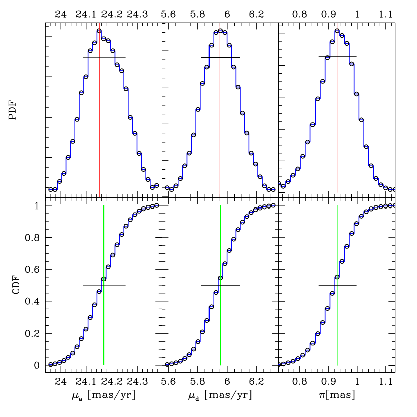
Figure 2.— Uncertainties in astrometric parameters as estimated by the bootstrap method for PSR B2310+42. The top row shows histograms of the estimates for the fit parameters from 50,000 bootstrap iterations, equivalent to an un-normalized probability distribution function (PDF), and the vertical line indicates the most common value (the mode). The bottom row shows the cumulative distribution function (CDF) derived from the histogram above, and the vertical line indicates the median parameter value. In each panel, the horizontal bar indicates the most compact 68.26% confidence interval (i.e., the smallest interval that includes 34,130 estimates for each given parameter). In this and every other case, the median and mode are consistent to well within the 68% confidence interval. The proper motion in right ascension, $\mu_{\alpha}$, is the angular rate, $\frac{d\alpha}{dt}\cos\delta$.

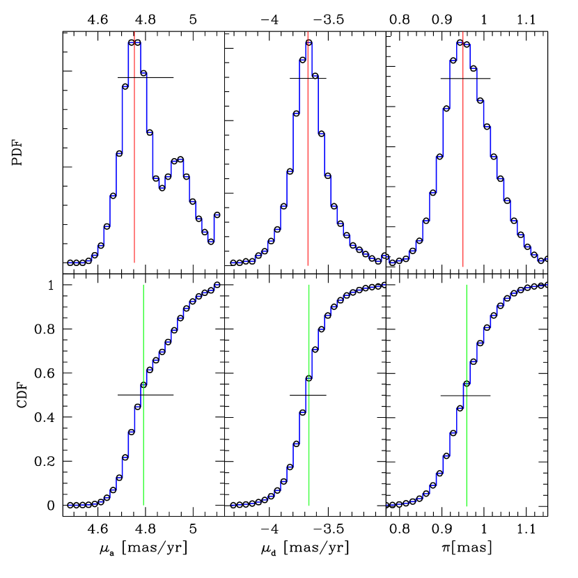
Figure 3.— Uncertainties in astrometric parameters as estimated by the bootstrap method for PSR J1713+0747. As in Figure 2, the top row shows the histogram of the estimates (equivalent to an un-normalized PDF) and the bottom row shows the cumulative distribution function (CDF) for each astrometric parameter, while vertical lines indicate the mode and median estimates and horizontal bars show the most compact 68% confidence interval for each parameter. The fit for $\mu_{\alpha}$ is the only case among all pulsars discussed in the present work where a bimodal distribution was obtained for an astrometric parameter, and thus represents our worst-case scenario. However, our astrometric results for this pulsar can be compared to independent estimates from pulse timing: see §6.3 and Table 4 for a discussion.

In all cases, the values of the parameters estimated by the bootstrap method were consistent with the parameters obtained by simple least squares fitting (using all epochs without replacement) to well within the bootstrap 68% confidence interval. However, the uncertainties in the estimates of the astrometric parameters differed between the two methods. The power of the technique is illustrated by our worst-case scenario (PSR J1713+0747, Figure 3), which was the only case where a bimodal distribution was obtained for any of the parameters. The bimodality in $\mu_{\alpha}$ reflects the presence or absence of one well-measured position, and causes the uncertainties to deviate significantly from symmetry. However, there is no ambiguity in the most probable parameter values or in the bootstrap confidence intervals. Coincidentally, PSR J1713+0747 has well determined astrometry from pulse timing as well, allowing a stringent check on our results, as we discuss further below (§6.3).

Table 2Astrometry Results

Pulsar	RA	Dec	$\mu_{\alpha}$	$\mu_{\delta}$	$\pi$
	(J2000)	(J2000)	(mas yr-1)	(mas yr-1)	(mas)
B0031$-$07	$00:34:08.8703(1)$	$-07:21:53.409(2)$	$10.37^{+0.08}_{-0.08}$	$-11.13^{+0.11}_{-0.16}$	$0.93^{+0.08}_{-0.07}$
B0136+57	$01:39:19.7401(12)$	$+58:14:31.819(17)$	$-19.11^{+0.06}_{-0.07}$	$-16.60^{+0.06}_{-0.07}$	$0.37^{+0.04}_{-0.04}$
B0450$-$18	$04:52:34.1057(1)$	$-17:59:23.371(2)$	$8.89^{+1.60}_{-2.24}$	$10.65^{+1.87}_{-1.29}$	$0.65^{+1.40}_{-0.59}$
B0450+55	$04:54:07.7506(1)$	$+55:43:41.437(2)$	$53.34^{+0.06}_{-0.05}$	$-17.56^{+0.12}_{-0.14}$	$0.84^{+0.04}_{-0.05}$
J0538+2817	$05:38:25.0572(1)$	$+28:17:09.161(2)$	$-23.57^{+0.10}_{-0.10}$	$52.87^{+0.09}_{-0.10}$	$0.72^{+0.12}_{-0.09}$
B0818$-$13	$08:20:26.3817(1)$	$-13:50:55.859(2)$	$21.64^{+0.09}_{-0.09}$	$-39.44^{+0.04}_{-0.05}$	$0.51^{+0.03}_{-0.04}$
B1508+55	$15:09:25.6298(1)$	$+55:31:32.394(2)$	$-73.64^{+0.05}_{-0.04}$	$-62.65^{+0.09}_{-0.08}$	$0.47^{+0.03}_{-0.03}$
B1541+09	$15:43:38.8250(1)$	$+09:29:16.339(2)$	$-7.61^{+0.06}_{-0.05}$	$-2.87^{+0.06}_{-0.07}$	$0.13^{+0.02}_{-0.02}$
J1713+0747	$17:13:49.5306(1)$	$+07:47:37.519(2)$	$4.75^{+0.17}_{-0.07}$	$-3.67^{+0.16}_{-0.15}$	$0.95^{+0.06}_{-0.05}$
B1933+16	$19:35:47.8259(1)$	$+16:16:39.986(2)$	$1.13^{+0.12}_{-0.13}$	$-16.09^{+0.15}_{-0.13}$	$0.22^{+0.08}_{-0.12}$
B2045$-$16	$20:48:35.6013(2)$	$-16:16:44.534(3)$	$113.16^{+0.02}_{-0.02}$	$-4.60^{+0.28}_{-0.23}$	$1.05^{+0.03}_{-0.02}$
B2053+36	$20:55:31.3521(1)$	$+36:30:21.469(2)$	$1.04^{+0.04}_{-0.04}$	$-2.46^{+0.13}_{-0.13}$	$0.17^{+0.03}_{-0.03}$
B2154+40	$21:57:01.8495(1)$	$+40:17:45.986(2)$	$16.13^{+0.09}_{-0.10}$	$4.12^{+0.12}_{-0.12}$	$0.28^{+0.06}_{-0.06}$
B2310+42	$23:13:08.6209(1)$	$+42:53:13.043(2)$	$24.15^{+0.10}_{-0.07}$	$5.95^{+0.13}_{-0.12}$	$0.93^{+0.06}_{-0.07}$

Note. — Pulsar coordinates have been adjusted for improvements in primary calibrator positions. Uncertainties in these coordinates (in parentheses) reflect uncertainties in the positions of primary calibrator; a minimum uncertainty of 0.0001 second of time in right ascension and 2 mas in declination are assigned as calibrator source structure evolution with frequency could cause systematic offsets from the reported 8.4 GHz positions at about this level. In all cases this calibrator position uncertainty is thought to be greater than the relative error introduced in phase-referencing. Quoted proper motion and parallax uncertainties are most compact 68% confidence intervals. All astrometry is performed and reported in Equinox J2000. Reported positions are for epoch 2002.0.

Table 3Parameters derived from astrometry

Pulsar	$l$	$b$	DM	$D_{DM}$	$D_{\pi}$	$V_{\perp}$
	(°)	(°)	(pc cm-3)	(kpc)	(kpc)	(km s-1)
B0031$-$07	110.42	$-$69.82	11.38	0.4	$1.06^{+0.08}_{-0.09}$	$77^{+6}_{-6}$
B0136+57	129.22	$-$4.04	73.78	2.8	$2.65^{+0.35}_{-0.26}$	$319^{+42}_{-33}$
B0450$-$18	217.08	$-$34.09	39.90	2.4	$0.76^{+0.36}_{-0.60}$	$54^{+23}_{-45}$
B0450+55	152.62	7.55	14.50	0.7	$1.19^{+0.07}_{-0.06}$	$317^{+19}_{-15}$
J0538+2817	179.72	$-$1.69	39.57	1.2	$1.30^{+0.22}_{-0.16}$	$357^{+59}_{-43}$
B0818$-$13	235.89	12.59	40.94	2.0	$1.96^{+0.17}_{-0.12}$	$418^{+36}_{-25}$
B1508+55	91.33	52.29	19.61	1.0	$2.10^{+0.13}_{-0.14}$	$963^{+61}_{-64}$
B1541+09	17.81	45.78	35.24	$>$35	$7.2^{+1.3}_{-1.1}$	$277^{+52}_{-42}$
J1713+0747	28.75	25.22	15.99	0.9	$1.05^{+0.06}_{-0.07}$	$30^{+2}_{-2}$
B1933+16	52.44	$-$2.09	158.52	5.6	$5.2^{+1.5}_{-2.7}$	$394^{+108}_{-208}$
B2045$-$16	30.51	$-$33.08	11.46	0.6	$0.95^{+0.02}_{-0.02}$	$512^{+13}_{-12}$
B2053+36	79.13	$-$5.59	97.31	4.6	$5.5^{+1.2}_{-0.8}$	$69^{+15}_{-11}$
B2154+40	90.49	$-$11.34	70.86	3.7	$3.4^{+0.9}_{-0.7}$	$264^{+73}_{-52}$
B2310+42	104.41	$-$16.42	17.28	1.2	$1.06^{+0.08}_{-0.07}$	$125^{+10}_{-8}$

Note. — Pulsar distances $D_{DM}$ were estimated from their dispersion measure (DM) using the NE2001 electron density model (Cordes & Lazio 2002). Confidence intervals for the parallax distances $D_{\pi}$ and transverse velocities $V_{\perp}$ were estimated directly from the bootstrap.

Compared to simple least squares fitting, the bootstrap method is expected to return larger fit uncertainties, since the time sampling for each trial in the bootstrap process is generally worse than simply using all epochs of data in the fit process. To compare the performance of the bootstrap method to simple least squares fitting, we simulated observations of PSR J1713+0747 on the actual observation dates, and recovered astrometric parameters both by a least squares fit to all the data, and by bootstrap. As expected, for Gaussian random uncertainties in the input position at each epoch, the two methods returned astrometric parameters that were essentially identical, differing by much less than the fit uncertainties, and the bootstrap method returned somewhat larger confidence intervals compared to the simple least squares fit (between 0 and 25%). Next, we added unmodeled systematic errors to the simulated positions, such that the mean “observed” position at a given epoch differed from the “true” position and the observation uncertainties understated the effective simulated errors. As systematic errors were added to increasing numbers of epochs, the results of the two techniques began to diverge. While the recovered best-fit astrometric parameters did not differ significantly between the two methods, the bootstrap fit uncertainty intervals generally encompassed the “true” parameter values (within 1- or 2-$\sigma$) while the simple least squares method returned uncertainties that were too optimistic and failed to include the input values within several multiples of $\sigma$ with increasing systematic errors. These simulations therefore justify our decision to use the bootstrap method when we are not able to reliably quantify the systematic errors in our observations; while our astrometry may be somewhat less precise as a result, it is more likely to be more accurate.

For illustration purposes, we show the parallax and proper motion signature of PSR B1933+16 in Figure 4, and the parallax signature of PSRs B0818$-$13 and B2310+42 in Figure 5. In these figures, the position error bars include estimates of the systematic error from the scatter between positions measured at each epoch at different frequency bands. However, we note that these estimates are used only for illustrative purposes, and the fit uncertainties are obtained from bootstrap, as described above.

Figure 4.— The proper motion and parallax of PSR B1933+16. The best fit parallax and proper motion ($\mu_{\alpha}=1.1$ mas yr^-1, $\mu_{\delta}=-16.1$ mas yr^-1, $\pi=0.2$ mas) is overplotted. The earliest position (top left) is at MJD 52485, while the final position (bottom right) is at MJD 53116. $\Delta$RA is the angular displacement $\Delta\alpha\,\cos\delta$. Note the different scales on the two axes.

Figure 5.— The parallax signature of two pulsars in Right Ascension and Declination, after subtracting the respective best-fit proper motions from the astrometric positions. $\Delta$RA is the angular displacement $\Delta\alpha\,\cos\delta$. Left: The parallax of PSR B0818$-$13, with curves overplotted corresponding to the best fit parallax $\pi=0.51$ mas. Right: The parallax of PSR B2310+42, with curves overplotted corresponding to the best fit parallax $\pi=0.93$ mas. In each panel, the inner error bars indicate the random position uncertainties, while the outer error bars indicate the net estimated uncertainties (random and systematic, added in quadrature) for illustration purposes only.

Finally, we note that signal-to-noise considerations required the averaging of all frequency bands for PSR B0450$-$18. As such, the bootstrap was performed with only 8 position measurement pairs ($\alpha_{t},\delta_{t}$ at each epoch) while fitting for 5 astrometric parameters, resulting in a high proportion of degenerate samples. For this one object, we repeated the bootstrap for $10^{6}$ iterations, but obtained no difference in the results or their confidence intervals compared to $10^{5}$ iterations. However, the uncertainties for the astrometric parameters for PSR B0450$-$18 are much larger than for the rest of our sample.

6. Discussion

We have presented parallaxes and proper motions for 14 pulsars (Table 2) and derived estimates for their distances and transverse velocities (Table 3). These results represent a significant increase in the number of pulsars with trigonometric parallaxes, and include distances to two pulsars over 5 kpc away that are determined to better than $\sim$15% : most probable $D=7.2^{+1.3}_{-1.1}$ kpc for PSR B1541+09, and $5.5^{+1.2}_{-0.8}$ kpc for PSR B2053+36. Early results from this program were published for two objects in the sample, PSR B1508+55 (Chatterjee et al. 2005) and PSR J0538+2817 (Ng et al. 2007), but with a simpler, more ad hoc treatment of the systematic errors. The bootstrap approach followed here does not assume that errors at each epoch are normally distributed, a condition that is now appreciated to be rarely true in phase referenced astrometry at frequencies below 5 GHz, where the turbulent ionosphere dominates the phase-referencing errors. For situations with over-determined measurements, such as those presented here, the bootstrap method effectively results in discrepant data receiving a lower weight, and so the current results are more robust.

For PSR B1508+55, the astrometric parameters determined here are consistent with our previous work, and the potential birth site in the Cygnus OB associations is unchanged. Nor is the high estimated velocity ($V_{\perp}\approx 1000$ km s^-1; $V_{3d}\gtrsim 1100$ km s^-1) significantly altered. For PSR J0538+2817, the proper motion in declination received an adjustment of about 2 $\sigma$ when employing the bootstrap analysis, but the magnitude of the change is small (from $52.59\pm 0.13$ mas yr^-1 to $52.87^{+0.09}_{-0.10}$ mas yr^-1), and does not affect the conclusions of Ng et al. (2007). The results also remain consistent with the timing results of Kramer et al. (2003), but are much more precise. Below we discuss some of the implications of our new measurements, particularly for birth sites, kinematic ages, Galactic electron density models, and reference frame ties.

6.1. Pulsar Birth Sites and Kinematic Ages

Accurate astrometric measurements allow pulsars to be traced back through the Galaxy to potential birth sites (e.g. Hoogerwerf et al. 2000, 2001; Vlemmings et al. 2004). If a birth site can be identified, the three-dimensional birth velocity can be estimated, a kinematic age $\tau_{\rm kin}$ can be inferred, and a combination of the birth spin period and braking index can be constrained. A detailed analysis of the Galactic trajectories of all pulsars with precise astrometry is beyond the scope of this work and will be presented in future (Vlemmings et al., in prep.), but a preliminary assessment of the current sample of pulsars is presented here.

The trajectories of the pulsars in our sample (except the old, recycled pulsar J1713+0747) are shown in Figure 6 for three different values of the (unknown) radial velocity ($V_{\rm r}=-200,0$ and $+200$ km s^-1). The pulsar trajectories were calculated using the three component Stäckel potential from Famaey & Dejonghe (2003) with the scaling parameters as described in Vlemmings et al. (2004). Figure 6 also shows the positions and extent of the nearby OB associations from de Zeeuw et al. (1999) and a number of open clusters compiled from the WEBDA catalog with a distance $<5$ kpc and a well-defined age $<10$ Myr. We only plot those open clusters for which a pulsar trajectory crosses within $20$ pc of the cluster center on the sky, without accounting for the distance or the motion of the cluster itself. The motion of the cluster can be $\sim$ several hundred pc during the lifetime of a pulsar, and needs to be taken into account in a more detailed analysis. Although a number of pulsar trajectories pass close to the OB associations or open clusters on the sky, the pulsar distance is typically incompatible with an origin in the cluster or association. However, besides the earlier identification of the likely birth site of PSR B1508+55 in one of the Cygnus OB associations (Chatterjee et al. 2005), the coarse analysis performed here reveals the possible birth location of PSR B2045$-$16 in the open cluster NGC 6604, as discussed below.

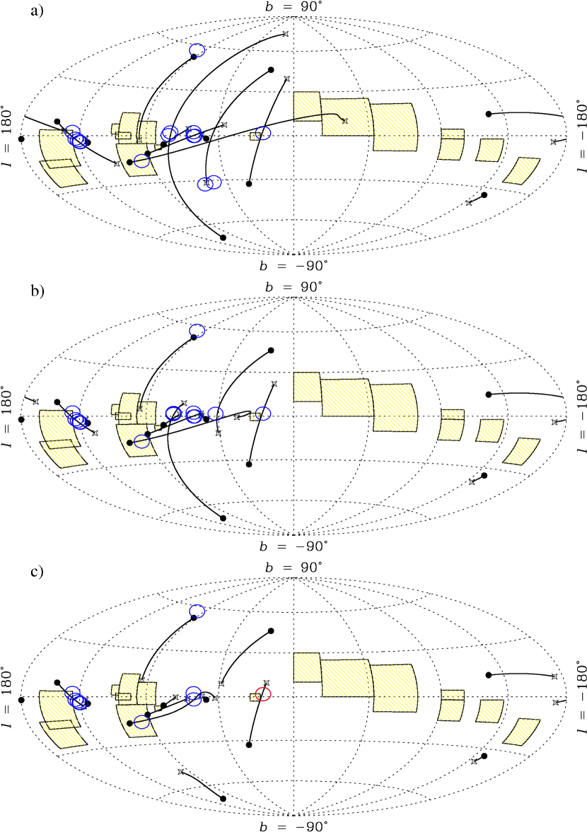
Figure 6.— The distribution of our pulsar sample in Galactic coordinates. The solid dots denote the present pulsar positions, and the lines represent their trajectory on the sky calculated for an age corresponding to the pulsar spin-down age. The open stars indicate the possible birth places of the pulsars. The three panels a,b and c represent the calculated orbits using $V_{r}=+200,0$ and $-200$ km s^-1 respectively. From left to right (decreasing $l$ of the present position) the pulsars are J0538+2817, B0450+55, B0136+57, B0031$-$07, B2310+42, B1508+55, B2154+40, B2053+36, B1933+16, B2045$-$16, B1541+09, B0818$-$13 and B0450$-$18. The shaded areas indicate the nearby OB associations (de Zeeuw et al. 1999). From left to right and from top to bottom: Per OB2, $\alpha$ Per, Cep OB3, Cep OB6, Cep OB2, Lac OB1, Cyg OB7, Cyg OB4, Sct OB2, Upper Sco, Upper Cen Lupus, Lower Cen Crux, Tr 10, Vela OB2, Col 121 and Ori OB1. The open circles denote the open clusters from the WEBDA catalog with well-defined distances ($<5$ kpc), positions and ages ($<50$ Myr). Only those open clusters are shown for which a pulsar orbit approaches the cluster position within $<20$ pc on the sky.

The progenitors of NS are massive O- and B-stars, which have a low Galactic scale height $\sim$63 pc, much smaller than the characteristic distance of radio pulsars from the Galactic plane. This is consistent with pulsars having significantly larger peculiar velocities than their progenitors, as recognized for example by Gott et al. (1970). As such, it is expected that most (young) pulsars should be moving away from the Galactic plane. Although Harrison et al. (1993) found that 17% of the young pulsars in their sample seemed to be moving towards the plane, later analysis indicates that after accounting for the pulsar birth scale height ($z_{0}=160\pm 40$ pc, Arzoumanian et al. 2002), all young pulsars do seem to be moving away from the Galactic plane (e.g., Cordes & Chernoff 1998; Brisken et al. 2003a; Hobbs et al. 2005). Any apparent motion toward the Galactic plane can often be explained by the unknown radial velocity $V_{\rm r}$, as the velocity perpendicular to the plane $V_{\rm z}$ is given by

$$V_{\rm z}=V_{\rm b}\cos{b}+V_{\rm r}\sin{b},$$ (1)

where $V_{\rm b}$ is the component of the velocity in the tangent plane along Galactic latitude $b$.

Alternatively, pulsars older than $\sim 20$ Myr could potentially already be falling back towards the plane due to the effect of the Galactic potential on their trajectory. Figure 7 indicates $V_{\rm z}$ against the location with respect to the Galactic plane for the pulsars in our sample. It is apparent that for a reasonable range of $V_{\rm r}$, all the pulsars are moving away from the Galactic plane, with the exception of PSR J0538+2817, which is located well within the pulsar birth scale height at $z=-41$ pc. Figure 7 also shows that, as expected, the youngest pulsars are found closest to the plane.

Assuming that all pulsars are indeed born in the Galactic plane between $-160<z_{0}<160$ pc, we can estimate the age of the pulsar from the measured $z=D\sin{b}$ and $V_{\rm z}$. The kinematic age $\tau_{\rm kin}$ is given by:

$$\tau_{\rm kin}=(D\sin{b}-z_{0})/V_{\rm z}.$$ (2)

The estimated kinematic ages of the pulsars in our sample are shown in Figure 8, for $-200<V_{\rm r}<+200$ km s^-1. As deceleration in the Galactic potential will reduce $V_{\rm z}$ as pulsars get older, $\tau_{\rm kin}$ will be a lower limit on the true age. Spin-down ages $\tau_{\rm sd}=P/2\dot{P}$ are also shown for comparison in Figure 8, where $P$ is the period of the pulsar, assumed to have been born spinning rapidly and slowing steadily with a braking index $n=3$. Each of these assumptions (rapid spin at birth, steady slowdown, $n=3$) is known to be problematic in specific cases (e.g., Gaensler & Frail 2000; Kramer et al. 2003). However, in spite of the variety of assumptions built into both $\tau_{\rm sd}$ and $\tau_{\rm kin}$, the agreement between them for most of the pulsars in our sample is remarkable.

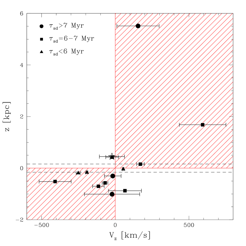
Figure 7.— Pulsar distance above the Galactic plane ($z$) versus its velocity perpendicular to the plane ($V_{\rm z}$). The different symbols represent different ranges of pulsar spin-down age and the open star indicates the recycled pulsar J1713+0747. As $V_{\rm z}$ depends on the unknown radial velocity of the pulsar, the bars denote $-200<V_{\rm r}<+200$ km s^-1. The pulsars in the shaded areas are moving away from the Galactic plane while those in the open areas are falling towards the plane. The horizontal dashed lines indicate the pulsar birth scale height determined by Arzoumanian et al. (2002).

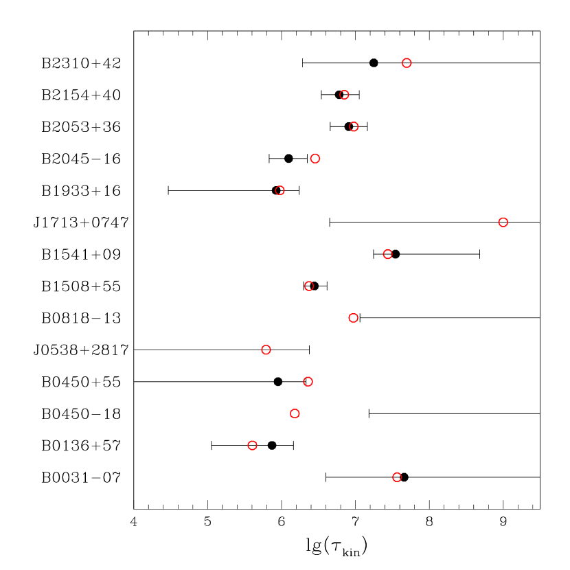
Figure 8.— Kinematic ages for our pulsar sample. The solid symbols denote the kinematic ages calculated using the pulsar distance above the Galactic plane and velocity $V_{\rm z}$, assuming $V_{\rm r}=0$ km s^-1. The bars indicate the range $-200<V_{\rm r}<+200$ km s^-1. The open circles are the spin-down ages. For those pulsars without solid symbols, the perpendicular velocity is pointing towards the plane when $V_{\rm r}=0$ km s^-1. As deceleration in the Galactic potential will have affected $V_{\rm z}$ for the pulsars older than $\sim 10$ Myr, $\tau_{\rm kin}$ will be a lower limit.

The only pulsars for which there is an apparent discrepancy between the two age estimates are PSRs J1713+0747, B0818$-$13, J0538+2817 and B0450$-$18. These pulsars appear to be falling towards the Galactic plane and thus have undetermined $\tau_{\rm kin}$ for $V_{\rm r}=0$. The recycled pulsar J1713+0747 has likely already completed one or more orbits through the Galactic plane, and the simple analysis outlined above is obviously inapplicable in that case. Allowing a radial velocity slightly larger than the arbitrary cutoff of 200 km s^-1 resolves the discrepancy for PSR B0818$-$13. PSR J0538+2817 is still within the Galactic pulsar birth scale height, as indicated above. It is associated with the known supernova remnant S147, and the pulsar age of $\sim 30$ kyr derived from the association (Kramer et al. 2003) is also quite inconsistent with its spin-down age ($\tau_{\rm sd}=620$ kyr). PSR B0450$-$18 requires $V_{r}\gtrsim 360$ km s^-1 at its most probable distance inferred from bootstrap ($D=0.76$ kpc), which may not be unreasonable, but in any case it has the largest uncertainties among the objects in our sample (c.f. §5).

6.1.1 PSR B2045$-$16

In our analysis of pulsar trajectories, PSR B2045$-$16 was found to pass on the sky within $\sim 20$ pc of the open cluster NGC 6604 for a radial velocity $V_{\rm r}\approx-200$ km s^-1. Since the distance between the cluster and the pulsar was also $\lesssim 20$ pc, NGC 6604 could be the birth location of PSR B2045$-$16. If it was born in this cluster, the kinematic age of PSR B2045$-$16 is $\tau_{\rm kin}\approx 1.9$ Myr, slightly less than its spin-down age $\tau_{\rm sd}=2.85$ Myr. NGC 6604 is an open cluster with an age $\sim 6.5$ Myr (Kharchenko et al. 2005). We infer that the progenitor of PSR B2045$-$16 was probably more massive than $\sim 20$ M_⊙ and that the birth velocity of the pulsar was $\sim 575$ km s^-1. Furthermore, the mismatch between the spin-down age and kinematic age can be resolved if the initial spin period of the pulsar was $P_{0}\sim 360$ ms, assuming a fixed braking index $n=3$, consistent with the population birth spin period distribution ($300\pm 150$ ms) found by Faucher-Giguère & Kaspi (2006). Alternatively, if the initial spin period is assumed to be much smaller than its current period, the kinematic age implies a braking index $n\approx 4$, which is larger than all measured values to date and thus an unlikely explanation. Further analysis will need to confirm the association of PSR B2045$-$16 with NGC 6604, taking into account the proper motion of NGC 6604 ($\mu_{\alpha}=-0.36$ mas yr^-1, $\mu_{\delta}=-2.68$ mas yr^-1 Kharchenko et al. 2005), which corresponds to a motion on the sky of $\sim 60$ pc in 2 Myr.

6.2. Electron Density Models

Model independent distances to pulsars provide essential calibration points for models of the Galactic electron density distribution such as NE2001 (Cordes & Lazio 2002), and one of the objectives of our observations is to use new pulsar distances to improve successors to NE2001. We have compared our astrometric distance estimates with those obtained from NE2001, as illustrated in Figure 9. In constructing NE2001, Cordes & Lazio (2002) estimated the uncertainty in the distances derived from the pulse dispersion measure (DM) to be 20%. For the purposes of our comparison, we do not include the NE2001 uncertainty estimate, but consider only whether the NE2001 distance estimate is within the 68% and 99% confidence intervals of the parallax distance.

Figure 9.— Comparison of distance estimates from dispersion measure and parallax distances for the objects in our sample as a function of (top panel) absolute Galactic latitude $|b|$ and (bottom panel) dispersion measure $\int_{0}^{D}n_{e}\,dl$. Dispersion measure distances are from NE2001 (Cordes & Lazio 2002) except for PSR B1541+09, for which NE2001 provides only a lower limit on the distance (see discussion in §6.2), and we have used an earlier distance estimate from Taylor & Cordes (1993). Error bars reflect only the uncertainties in the distance estimated from parallax, and PSR B0450$-$18 has been excluded from the plot due to the large uncertainties. It is apparent that NE2001 underestimates distances to some of the pulsars in our sample at high Galactic latitudes, consistent with a larger scale height or irregularities in the ISM at the relevant scales.

Of the 14 pulsars in our sample, the NE2001 distance estimates are in approximate agreement with our parallax determinations (within or just beyond the 68% confidence intervals) for 9 of the pulsars. The other five pulsars (B0031$-$07, B1508+55, B2045$-$16, B1541+09, and B0450+55) are discussed below.

Three of the discrepant pulsars (B0031$-$07 (catalog PSR), B1508$+$55 (catalog PSR), and B2045$-$16 (catalog PSR)) have high Galactic latitudes $|b|>30\arcdeg$ and low DMs $\mathrm{DM}<20$ pc cm^-3. The NE2001 model contains a set of low electron density components designed to reproduce the effects of local Galactic structure, namely regions such as the Local Hot Bubble (LHB), a local Low Density Region (LDR), and the Local Superbubble (LSB). The distances to these three pulsars are large enough that none are within any of these local, low-density regions. Thus, these local structures cannot be the explanation for the systematic discrepancies.

Gaensler et al. (2008) have re-analyzed the available DM data toward high Galactic latitude pulsars and find that the scale height of the ionized gas is approximately 1.8 kpc, about a factor of 2 higher than the thick disk component in the NE2001 model. Analyzing the DM data in combination with emission measures (EM) derived from H$\alpha$ observations, they also conclude that the filling factor of the ionized gas increases with distance above the Galactic plane.

Using the Gaensler et al. (2008) re-assessment for the ionized gas scale height, we have estimated the distances to these pulsars from their DMs. In general, the resulting distances are slight over-estimates relative to their parallax distances. We conclude that the new parallax distances and the DMs of these pulsars are consistent with the conclusion of Gaensler et al. (2008) of a larger scale height for the ionized gas, though their estimated scale height of 1.8 kpc may be a bit too high. A revised fit including the new distances presented here indeed yields a slightly lower scale height (B. M. Gaensler, personal communication), but does not significantly alter the conclusions of Gaensler et al. (2008). We note, however, that the ISM is likely to be significantly irregular or patchy on the relevant length scales, particularly at high Galactic latitudes, where chimmneys and voids are important contributors to the structure.

PSR B1541$+$09 (catalog PSR) is also at high Galactic latitude ($b=45\arcdeg$) but has a relatively large DM (35.24 pc cm^-3). This DM is above the maximal value ($\approx 30$ pc cm^-3) from the thick disk component in the NE2001 model, which only provides lower limits on the pulsar distance. Thus, in order to reproduce the DM, the NE2001 model includes a “clump” of enhanced electron density (contributing about 10% of the total DM), though Cordes & Lazio (2002) could find no obvious feature along the line of sight that might generate this clump (e.g., an H II region or O star). This line of sight also passes above two spiral arms in the NE2001 model. One possibility is that the scale height of the ionized gas above one or both of these arms is larger than included in the model.

Lastly, PSR B0450$+$55 (catalog PSR) lies at a relatively low Galactic latitude ($b=7\fdg 5$), with DM $=14.495$ pc cm^-3. At the parallax distance to the pulsar, the DM inferred from the NE2001 model is 33 pc cm^-3, much larger than what is observed. The situation can plausibly be explained by a deficit of electrons in this direction. Within the NE2001 model, there are attempts to account for such deficits (“voids”) in the electron density along specific lines of sight, but such modeling is limited by the sparseness of available DM-independent distance estimates.

We have examined both the Virginia Tech Spectral-Line Survey H-$\alpha$ image and the WHAM H-$\alpha$ survey (Haffner et al. 2003); neither shows any indication that the line of sight toward the pulsar has any deficit of H-$\alpha$ emission compared to nearby lines of sight. However, a CO survey (Dame et al. 2001) shows a tongue of CO emission that crosses the line of sight to the pulsar. While the filling factor of the CO gas along the line of sight to the pulsar may not be large, its presence suggests that not all of the line of sight may be ionized, consistent with an apparent void in the electron density along the line of sight to this pulsar.

6.3. Reference Frame Ties

Pulse timing provides radio pulsar positions in the Solar system reference frame, while VLBI measurements are tied to the distant quasars. Simply measuring precise positions for pulsars via the two different techniques enables fundamental reference frame ties between the Solar system and the extragalactic ICRF (e.g. Bartel et al. 1996). The recycled pulsar J1713+0747 is now one of two pulsars (along with PSR J0437$-$4715; Deller et al. 2008) with high-precision astrometry and statistically significant measurements of parallax using both pulse timing and VLBI. In Table 4 we list the astrometric parameters for PSR J1713+0747 as determined by interferometry (this work) as well as by two independent pulse timing efforts (Splaver et al. 2005; Hotan et al. 2006).

Table 4Astrometry for PSR J1713+0747

Measurement	VLBA	Splaver et al.	Hotan et al.
$\Delta\alpha$ (s)	0.5306(1)	0.5307826(7)	0.53077(1)
$\Delta\delta$ (″)	0.519(2)	0.52339(3)	0.5228(2)
$\mu_{\alpha}$ (mas yr-1)	4.75${}^{+17}_{-7}$	4.917(4)	4.97(6)
$\mu_{\delta}$ (mas yr-1)	$-$3.67(16)	$-$3.933(10)	$-$3.7(1)
$\pi$ (mas)	0.95(6)	0.89(8)	1.1(1)

Note. — Astrometric parameters for PSR J1713+0747 from VLBA astrometry (this work) are compared to parameters derived independently from pulse timing (Splaver et al. 2005; Hotan et al. 2006). All parameters are for equinox J2000; positions are shifted to match the VLBI data epoch of year 2002.0 (MJD 52275) and listed as offsets from RA $17^{\mathrm{h}}13^{\mathrm{m}}49^{\mathrm{s}}$ ($\Delta\alpha$), Dec $07^{\circ}37^{\prime}47^{\prime\prime}$ ($\Delta\delta$).

The data used by Splaver et al. (2005) span 12 years (though with a 4 year gap), allowing compensation for timing noise. In contrast, Hotan et al. (2006) used data spanning only 2.5 years, which did not allow corrections for timing noise, but allowed them to minimize systematics through the consistency of their instrumental setup. We note that the overall consistency between the timing and VLBI results for proper motion and parallax is quite good, although the position differs in Declination at the $\sim$mas level. The longer time series allows Splaver et al. (2005) to attain higher precision in their proper motion estimates, but the uncertainties in parallax are comparable between the 12 year timing data set and the 2 year VLBI data, illustrating the complementarity of the techniques. An ensemble of such measurements on recycled pulsars has great promise for reference frame ties, as well as for the detection of gravitational waves.

7. Conclusions

By simply measuring the positions of neutron stars over time to high accuracy, it is possible to establish constraints on a variety of scientific questions. Here we have presented the motivation, methods, and results from a large VLBA astrometry program. We have described our initial VLA surveys to select targets and find in-beam calibrators, as well as VLBA observations, pulsar gating, and data reduction. We have identified a few specific pitfalls, including proximity of the targets to the Sun, and the widespread presence of satellite-generated RFI. We have also described the use of the bootstrap method to comprehensively treat unmodeled systematic errors. The methods described here are serving as templates for our ongoing astrometry programs, and may serve as useful guidelines for the wider community.

As a result of our VLBA astrometry program, we have measured new parallaxes and proper motions for 14 pulsars, including $\pi=0.13^{+0.02}_{-0.02}$ mas for PSR B1541+09. The measurements have been exploited to investigate their kinematics and birth sites. Young pulsars are found to be leaving the Galactic plane, as expected, and we also find that spindown ages and kinematic ages are generally in reasonable agreement, with some notable exceptions. We have identified a plausible birth site for PSR B1508+55 in one of the Cyg OB associations (Chatterjee et al. 2005) and for PSR B2045$-$16 in the open cluster NGC 6604 (this work).

The new model-independent distances have also allowed us to revisit models of the Galactic electron density distribution. Comparing distance estimates from parallax and pulse dispersion measure, we find that NE2001 underestimates distances for some objects at high Galactic latitudes, while for others the estimates agree with or are larger than the parallax distances. Our findings are consistent with a larger scale height or with irregularities in the ISM on relevant length scales. Independent distance measurements are essential to calibrate models and probe structure in the ISM, and the present sample will be incorporated into future iterations of the electron density distribution model, ultimately improving DM-based distance estimates for all pulsars.

Finally, we have compared our precise astrometry on the recycled pulsar J1713+0747 with two independent results from pulse timing. The comparison can be used to verify consistency between the extragalactic ICRF and the Solar system reference frame, especially as part of an ensemble of recycled pulsars.

The Very Long Baseline Array is the only instrument that offers full-time, dedicated VLBI capabilities. Our results once again illustrate the power of the instrument to provide astrometry even at lower frequencies with high precision and excellent accuracy.

References

- Arras & Lai (1999) Arras, P., & Lai, D. 1999, ApJ, 519, 745
- Arzoumanian et al. (2002) Arzoumanian, Z., Chernoff, D. F., & Cordes, J. M. 2002, ApJ, 568, 289
- Bartel et al. (1996) Bartel, N., Chandler, J. F., Ratner, M. I., Shapiro, I. L., Pan, R., & Cappallo, R. J. 1996, AJ, 112, 1690
- Beasley et al. (2002) Beasley, A. J., Gordon, D., Peck, A. B., Petrov, L., MacMillan, D. S., Fomalont, E. B., & Ma, C. 2002, ApJS, 141, 13
- Blazek et al. (2006) Blazek, J. A., Gaensler, B. M., Chatterjee, S., van der Swaluw, E., Camilo, F., & Stappers, B. W. 2006, ApJ, 652, 1523
- Bridle & Schwab (1999) Bridle, A. H., & Schwab, F. R. 1999, in Astronomical Society of the Pacific Conference Series, Vol. 180, Synthesis Imaging in Radio Astronomy II, ed. G. B. Taylor, C. L. Carilli, & R. A. Perley, 371–+
- Briggs et al. (1999) Briggs, D. S., Schwab, F. R., & Sramek, R. A. 1999, in Astronomical Society of the Pacific Conference Series, Vol. 180, Synthesis Imaging in Radio Astronomy II, ed. G. B. Taylor, C. L. Carilli, & R. A. Perley, 127–+
- Brisken et al. (2000) Brisken, W. F., Benson, J. M., Beasley, A. J., Fomalont, E. B., Goss, W. M., & Thorsett, S. E. 2000, ApJ, 541, 959
- Brisken et al. (2002) Brisken, W. F., Benson, J. M., Goss, W. M., & Thorsett, S. E. 2002, ApJ, 571, 906
- Brisken et al. (2003a) Brisken, W. F., Fruchter, A. S., Goss, W. M., Herrnstein, R. M., & Thorsett, S. E. 2003a, AJ, 126, 3090
- Brisken et al. (2003b) Brisken, W. F., Thorsett, S. E., Golden, A., & Goss, W. M. 2003b, ApJ, 593, L89
- Burrows & Hayes (1996) Burrows, A., & Hayes, J. 1996, Physical Review Letters, 76, 352
- Chatterjee et al. (2001) Chatterjee, S., Cordes, J. M., Lazio, T. J. W., Goss, W. M., Fomalont, E. B., & Benson, J. M. 2001, ApJ, 550, 287
- Chatterjee et al. (2004) Chatterjee, S., Cordes, J. M., Vlemmings, W. H. T., Arzoumanian, Z., Goss, W. M., & Lazio, T. J. W. 2004, ApJ, 604, 339
- Chatterjee et al. (2005) Chatterjee, S., Vlemmings, W. H. T., Brisken, W. F., Lazio, T. J. W., Cordes, J. M., Goss, W. M., Thorsett, S. E., Fomalont, E. B., Lyne, A. G., & Kramer, M. 2005, ApJ, 630, L61
- Cordes & Chernoff (1998) Cordes, J. M., & Chernoff, D. F. 1998, ApJ, 505, 315
- Cordes & Lazio (2002) Cordes, J. M., & Lazio, T. J. W. 2002, ArXiv e-print, astro-ph/0207156
- Cornwell & Perley (1992) Cornwell, T. J., & Perley, R. A. 1992, A&A, 261, 353
- Dame et al. (2001) Dame, T. M., Hartmann, D., & Thaddeus, P. 2001, ApJ, 547, 792
- De Luca et al. (2008) De Luca, A., Caraveo, P. A., Esposito, P., & Hurley, K. 2008, ArXiv e-prints, 0810.3804
- de Zeeuw et al. (1999) de Zeeuw, P. T., Hoogerwerf, R., de Bruijne, J. H. J., Brown, A. G. A., & Blaauw, A. 1999, AJ, 117, 354
- Deller et al. (2008) Deller, A. T., Verbiest, J. P. W., Tingay, S. J., & Bailes, M. 2008, ApJ, 685, L67
- Efron & Tibshirani (1991) Efron, B., & Tibshirani, R. 1991, Science, 253, 390
- Famaey & Dejonghe (2003) Famaey, B., & Dejonghe, H. 2003, MNRAS, 340, 752
- Faucher-Giguère & Kaspi (2006) Faucher-Giguère, C.-A., & Kaspi, V. M. 2006, ApJ, 643, 332
- Fey et al. (2004) Fey, A. L., Ma, C., Arias, E. F., Charlot, P., Feissel-Vernier, M., Gontier, A.-M., Jacobs, C. S., Li, J., & MacMillan, D. S. 2004, AJ, 127, 3587
- Fomalont et al. (1999) Fomalont, E. B., Goss, W. M., Beasley, A. J., & Chatterjee, S. 1999, AJ, 117, 3025
- Fomalont et al. (2006) Fomalont, E. B., Kellermann, K. I., Cowie, L. L., Capak, P., Barger, A. J., Partridge, R. B., Windhorst, R. A., & Richards, E. A. 2006, ApJS, 167, 103
- Fomalont et al. (2003) Fomalont, E. B., Petrov, L., MacMillan, D. S., Gordon, D., & Ma, C. 2003, AJ, 126, 2562
- Gaensler & Frail (2000) Gaensler, B. M., & Frail, D. A. 2000, Nature, 406, 158
- Gaensler et al. (2008) Gaensler, B. M., Madsen, G. J., Chatterjee, S., & Mao, S. A. 2008, ArXiv e-prints
- Gott et al. (1970) Gott, J. R. I., Gunn, J. E., & Ostriker, J. P. 1970, ApJ, 160, L91
- Gwinn et al. (1986) Gwinn, C. R., Taylor, J. H., Weisberg, J. M., & Rawley, L. A. 1986, AJ, 91, 338
- Haffner et al. (2003) Haffner, L. M., Reynolds, R. J., Tufte, S. L., Madsen, G. J., Jaehnig, K. P., & Percival, J. W. 2003, ApJS, 149, 405
- Harrison et al. (1993) Harrison, P. A., Lyne, A. G., & Anderson, B. 1993, MNRAS, 261, 113
- Helfand et al. (2007) Helfand, D. J., Chatterjee, S., Brisken, W. F., Camilo, F., Reynolds, J., van Kerkwijk, M. H., Halpern, J. P., & Ransom, S. M. 2007, ApJ, 662, 1198
- Hobbs et al. (2005) Hobbs, G., Lorimer, D. R., Lyne, A. G., & Kramer, M. 2005, MNRAS, 360, 974
- Hobbs et al. (2004) Hobbs, G., Lyne, A. G., Kramer, M., Martin, C. E., & Jordan, C. 2004, MNRAS, 353, 1311
- Hoogerwerf et al. (2000) Hoogerwerf, R., de Bruijne, J. H. J., & de Zeeuw, P. T. 2000, ApJ, 544, L133
- Hoogerwerf et al. (2001) —. 2001, A&A, 365, 49
- Hotan et al. (2006) Hotan, A. W., Bailes, M., & Ord, S. M. 2006, MNRAS, 369, 1502
- Janka & Mueller (1996) Janka, H.-T., & Mueller, E. 1996, A&A, 306, 167
- Johnston et al. (2005) Johnston, S., Hobbs, G., Vigeland, S., Kramer, M., Weisberg, J. M., & Lyne, A. G. 2005, MNRAS, 364, 1397
- Kaplan et al. (2008a) Kaplan, D. L., Chatterjee, S., Gaensler, B. M., & Anderson, J. 2008a, ApJ, 677, 1201
- Kaplan et al. (2008b) Kaplan, D. L., Chatterjee, S., Hales, C., Gaensler, B. M., & Slane, P. O. 2008b, ArXiv e-prints, 0810.4184
- Kaplan et al. (2002) Kaplan, D. L., van Kerkwijk, M. H., & Anderson, J. 2002, ApJ, 571, 447
- Kaplan et al. (2007) —. 2007, ApJ, 660, 1428
- Kharchenko et al. (2005) Kharchenko, N. V., Piskunov, A. E., Röser, S., Schilbach, E., & Scholz, R.-D. 2005, A&A, 438, 1163
- Kramer et al. (2003) Kramer, M., Lyne, A. G., Hobbs, G., Löhmer, O., Carr, P., Jordan, C., & Wolszczan, A. 2003, ApJ, 593, L31
- Lai et al. (2001) Lai, D., Chernoff, D. F., & Cordes, J. M. 2001, ApJ, 549, 1111
- Lattimer & Prakash (2004) Lattimer, J. M., & Prakash, M. 2004, Science, 304, 536
- Ma et al. (1998) Ma, C., Arias, E. F., Eubanks, T. M., Fey, A. L., Gontier, A.-M., Jacobs, C. S., Sovers, O. J., Archinal, B. A., & Charlot, P. 1998, AJ, 116, 516
- Migliazzo et al. (2002) Migliazzo, J. M., Gaensler, B. M., Backer, D. C., Stappers, B. W., van der Swaluw, E., & Strom, R. G. 2002, ApJ, 567, L141
- Ng & Romani (2007) Ng, C.-Y., & Romani, R. W. 2007, ApJ, 660, 1357
- Ng et al. (2007) Ng, C.-Y., Romani, R. W., Brisken, W. F., Chatterjee, S., & Kramer, M. 2007, ApJ, 654, 487
- Petrov et al. (2005) Petrov, L., Kovalev, Y. Y., Fomalont, E., & Gordon, D. 2005, AJ, 129, 1163
- Preston et al. (1983) Preston, R. A., Morabito, D. D., & Jauncey, D. L. 1983, ApJ, 269, 387
- Romney (1999) Romney, J. D. 1999, in Astronomical Society of the Pacific Conference Series, Vol. 180, Synthesis Imaging in Radio Astronomy II, ed. G. B. Taylor, C. L. Carilli, & R. A. Perley, 57–+
- Socrates et al. (2005) Socrates, A., Blaes, O., Hungerford, A., & Fryer, C. L. 2005, ApJ, 632, 531
- Spangler et al. (2002) Spangler, S. R., Kavars, D. W., Kortenkamp, P. S., Bondi, M., Mantovani, F., & Alef, W. 2002, A&A, 384, 654
- Splaver et al. (2005) Splaver, E. M., Nice, D. J., Stairs, I. H., Lommen, A. N., & Backer, D. C. 2005, ApJ, 620, 405
- Standish (1982) Standish, Jr., E. M. 1982, A&A, 114, 297
- Taylor & Cordes (1993) Taylor, J. H., & Cordes, J. M. 1993, ApJ, 411, 674
- Thorsett et al. (2002) Thorsett, S. E., Brisken, W. F., & Goss, W. M. 2002, ApJ, 573, L111
- Toscano et al. (1999) Toscano, M., Britton, M. C., Manchester, R. N., Bailes, M., Sandhu, J. S., Kulkarni, S. R., & Anderson, S. B. 1999, ApJ, 523, L171
- Verbiest et al. (2008) Verbiest, J. P. W., Bailes, M., van Straten, W., Hobbs, G. B., Edwards, R. T., Manchester, R. N., Bhat, N. D. R., Sarkissian, J. M., Jacoby, B. A., & Kulkarni, S. R. 2008, ApJ, 679, 675
- Vlemmings et al. (2004) Vlemmings, W. H. T., Cordes, J. M., & Chatterjee, S. 2004, ApJ, 610, 402
- Wall et al. (2005) Wall, J. V., Jackson, C. A., Shaver, P. A., Hook, I. M., & Kellermann, K. I. 2005, A&A, 434, 133
- Walter & Lattimer (2002) Walter, F. M., & Lattimer, J. M. 2002, ApJ, 576, L145
- Winkler & Petre (2007) Winkler, P. F., & Petre, R. 2007, ApJ, 670, 635
- Yakovlev & Pethick (2004) Yakovlev, D. G., & Pethick, C. J. 2004, ARA&A, 42, 169
- Zeiger et al. (2008) Zeiger, B. R., Brisken, W. F., Chatterjee, S., & Goss, W. M. 2008, ApJ, 674, 271