Unconventional Bose-Einstein Condensations Beyond the “No-node” Theorem

Abstract

Feynman’s “no-node” theorem states that the conventional many-body ground-state wavefunctions of bosons in the coordinate representation is positive-definite. This implies that time-reversal symmetry cannot be spontaneously broken. In this article, we review our progress in studying a class of new states of unconventional Bose-Einstein condensations beyond this paradigm. These states can either be the long-lived metal-stable states of ultra-cold bosons in high orbital bands in optical lattices as a result of the “orbital-Hund’s rule” interaction, or the ground states of spinful bosons with spin-orbit coupling linearly dependent on momentum. In both cases, Feynman’s argument does not apply. The resultant many-body wavefunctions are complex-valued and thus break time-reversal symmetry spontaneously. Exotic phenomena in these states include the Bose-Einstein condensation at non-zero momentum, the ordering of orbital angular momentum moments, the half-quantum vortex, and the spin texture of skyrmions.

1 Introduction

In Feynman’s statistical mechanics textbook, it is stated that the many-body ground state wavefunctions of bosons are positive-definite in the coordinate representation provided no external rotation is applied and interactions are short-ranged [1]. The proof is very intuitive: due to the time-reversal (TR) symmetry, the ground state wavefunction $\Psi(\vec{r}_{1},....,\vec{r}_{n})$ can be chosen as real. If it is not positive-definite, i.e., it has nodes, the following surgery can be done to lower its energy. We first take its absolute value of $|\Psi(\vec{r}_{1},....,\vec{r}_{n})|$, whose energy expectation value is exactly the same as that of $\Psi(\vec{r}_{1},....,\vec{r}_{n})$. However, such a wavefunction has kinks at node points. Further smoothing the kinks results in a positive-definite wavefunction, and the kinetic energy is lowered by softening the gradients of the wavefunction. Although the single body potential energy and the two-body interaction energy increase, they are small costs of a high order compared to the gain of the kinetic energy. We can further conclude that the ground state is non-degenerate because two degenerate positive-definite wavefunctions cannot be orthogonal to each other.

This “no-node” theory is a very general statement, which applies to almost all the well-known ground states of bosons, including the superfluid, Mott-insulating, density-wave, and even super-solid ground states. It is also a very strong statement, which reduces the generally speaking complex-valued many-body wavefunctions to be positive-definite distributions. This is why the ground state properties of bosonic systems, such as ⁴He, can in principle be exactly simulated by the quantum Monte-Carlo method free of the sign problem. Furthermore, this statement implies that the ordinary ground states of bosons, including Bose-Einstein condensations (BEC) and Mott-insulating states, cannot spontaneously break time-reversal (TR) symmetry, since TR transformation for the single component bosons is simply the operation of the complex conjugation.

It would be exciting to search for exotic emergent states of bosons beyond this “no-node” paradigm, whose many-body wavefunctions can be complex-valued with spontaneous TR symmetry breaking. Since properties of complex-valued functions are much richer than those of real-valued ones, we expect such states can exhibit more intriguing properties than the ordinary ground states of bosons. For this purpose, we have recently made much progress with two different ways to bypass Feynman’s argument, including the meta-stable states of bosons in the high orbital bands of optical lattices [2, 3, 4] and multi-component bosons with spin-orbit coupling linearly dependent on momentum [5].

Clearly, the “no-node” theorem is a ground state property which does not apply to the excited states of bosons. The recent rapid development of optical lattices with ultra-cold bosons provides a wonderful opportunity to investigate the meta-stable states of bosons pumped into high orbital bands. Due to the lack of dissipation channels, the life time can be long enough to develop inter-site coherence [6, 7]. We have shown that the interaction among orbital bosons are characterized by the “orbital Hund’s rule” [2, 3], which gives rise to a class of complex superfluid states by developing the on-site orbital angular momentum (OAM) moments. In the lattice systems, the inter-site hoppings of bosons lock the OAM polarization into regular patterns depending the concrete lattice structures.

Furthermore, the “no-node” theorem even does not apply to the ground states of bosons if their Hamiltonians linearly depend on momentum, i.e., the gradient operator. A trivial example is the formation of vortices in Bose condensates with the external rotation in which the Coriolis force is represented as the vector potential linearly coupled to momentum. However, in this case TR symmetry is explicitly broken. A non-trivial example is that bosons with spin-orbit (SO) coupling, whose Hamiltonians also linearly depend on momentum and are TR invariant. The invalidity of the “no-node” theorem can also give rise to complex-valued ground state wavefunctions.

Although ⁴He is spinless and most bosonic alkali atoms are too heavy to exhibit the relativistic SO coupling in their center-of-mass motion, SO coupling can be important in exciton systems in two dimensional quantum wells. We have shown that the Rashba SO coupling in the conduction electron bands induces the same type of SO coupling in the center-of-mass motion of excitons. In a harmonic trap, the ground state condensate wavefunction can spontaneously develop half-quantum vortex structure and the skyrmion type of the spin texture configuration [5]. On the other hand, effective SO coupling in boson systems can be induced by laser beams, which has been investigated in several publications by other groups in Refs [8, 9, 10, 11].

In the following, we will review our work in both directions outlined above including many new results unpublished before. In Section 2, we explain the characteristic feature of interacting bosons in high orbital bands, the “orbital Hund’s rule”, and the consequential complex-superfluid states with the ordering of on-site OAM moments. The ordering of OAM moments in the Mott-insulating states is also investigated. In Section 3, we review the TR symmetry breaking states of spinful bosons with spin-orbit coupling. Interesting properties including half-quantum vortex, and the skyrmion-like spin-textures are studied. Conclusions are made in Section 4.

Due to the limit of space, we will not cover interesting related topics of orbital bosons, such as the nematic superfluid state [6] and the algebraic superfluid state [12], and the orbital physics with cold fermions [13, 14, 15, 16, 17, 18, 19, 20], which has also aroused much research attention recently.

2 “Complex-condensation” of bosons in high orbital bands in optical lattices

In this section, we will review the “complex-condensation” with TR symmetry breaking, which is a new state of the $p$-orbital bosons. This is an example of novel orbital physics in optical lattice with cold bosons. Below let us give a brief general introduction to orbital physics for the general audience.

Orbital is a degree of freedom independent of charge and spin. It plays important roles in magnetism, superconductivity, and transport in transition metal oxides [21, 22, 23]. The key features of orbital physics are orbital degeneracy and spatial anisotropy. Optical lattices bring new features to orbital physics which are not easily accessible in solid state orbital systems. First, optical lattices are rigid lattices and free from the Jahn-Teller distortion, thus orbital degeneracy is robust. Second, the meta-stable bosons pumped into high orbital bands exhibit novel superfluidity beyond Feynman’s “no-node” theory [6, 2, 24, 3, 12, 25, 4]. Third, $p$-orbitals have stronger spatial anisotropy than that of $d$ and $f$-orbitals, while correlation effects in $p$-orbital solid state systems (e.g. semiconductors) are not that strong. In contrast, interaction strength in optical lattices is tunable. We can integrate strong correlation with spatial anisotropy more closely than ever in $p$-orbital optical lattice systems [13, 14, 15, 16, 17].

Recently, orbital physics with cold atoms has been attracting a great deal of attention[26, 6, 2, 24, 3, 12, 25, 13, 27, 28, 29, 30, 31, 7]. For orbital bosons, a series of theory works have been done [6, 26, 2, 24, 3, 12, 25, 4, 27], including the illustration of the ferro-orbital nature of interactions [2], orbital superfluidity with spontaneous time-reversal symmetry breaking [2, 3, 24, 4], the nematic superfluidity[6, 12]. The theory work on the $p$-orbital fermions is also exciting including the flat band and associated strong correlation physics in the honeycomb lattice [13, 15, 17], orbital exchange and frustration [16, 20], and topological insulators [14, 18].

The experimental progress has been truly exciting [29, 30, 31, 7]. Mueller et al. [7] have realized the meta-stable $p$-orbital boson systems by using the stimulated Raman transition. The spatially anisotropic phase coherence pattern has been observed in the time of flight experiments. Sebby-strabley et al. [31] have successfully pumped bosons into excited bands in the double-well lattice. In addition, $p$-orbital Bose-Einstein condensation (BEC) has also been observed in quasi one-dimensional exciton-polariton lattice systems [32].

Below we illustrate the important feature of interactions between orbital bosons, the “orbital Hund’s rule”, which results in TR symmetry breaking.

2.1 Orbital Hund’s rule of interacting orbital bosons

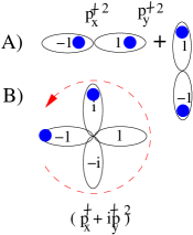
Figure 1: A single site problem with two spinless bosons occupying $p_{x,y}$-orbitals: (A) the OAM singlet and (B) one of the OAM doublets. The latter is energetically more favorable than the former as a result of the “orbital Hund’s rule”. The bonding pattern of $p$-orbitals: (C) the $\sigma$-bonding and (D) the $\pi$-bonding.

The most remarkable feature of interacting bosons in high orbital bands is that they favor to maximize their onsite orbital angular momentum (OAM) as explained below [2, 3].

Let us illustrate this Hund’s rule type physics through the simplest example: a single site problem with two degenerate $p_{x,y}$-orbitals filled with two spinless bosons. Because bosons are indistinguishable, the Hilbert space for the two-body states only contains three states, which can be classified according to their OAM: an OAM singlet as $\frac{1}{2}(p_{x}^{\dagger}p_{x}^{\dagger}+p_{y}^{\dagger}p_{y}^{\dagger})|0\rangle$ depicted in Fig 1. A, and a pair of OAM doublets $\frac{1}{2\sqrt{2}}(p^{\dagger}_{x}\pm ip^{\dagger}_{y})^{2}|0\rangle$ with $L_{z}=\pm 2$ as depicted in Fig 1 B. Assuming a contact interaction $V=g\delta(r_{1}-r_{2})$, the interaction energy of the former is calculated as $\frac{4}{3}U$ while that of the latter is $\frac{2}{3}U$ with the definition of

$$U=g\int dr^{2}|\psi_{p_{x}}(r)|^{4}=g\int dr^{2}|\psi_{p_{y}}(r)|^{4}.$$ (1)

In the OAM singlet state, bosons occupy polar (real) orbitals (e.g. $p_{x},p_{y}$), whose angular distribution in real space is narrower than that of the axial (complex) orbitals (e.g. $p_{x}\pm ip_{y}$ ) for the OAM doublets. By occupying the same axial orbital and therefore maximizing OAM, two bosons enjoy more room to avoid each other.

This “ferro-orbital” interaction is captured by the following multi-band Hubbard Hamiltonian for the $p$-orbital bosons as

$$H_{int}=\frac{U}{2}\sum_{\vec{r}}\big{\{}n^{2}_{\vec{r}}-\frac{1}{3}L_{z}^{2}\big{\}},$$ (2)

where $n=p^{\dagger}_{x}p_{x}+p^{\dagger}_{y}p_{y}$ and $L_{z}=-i(p^{\dagger}_{x}p_{y}-p^{\dagger}_{y}p_{x})$. The first term is the ordinary Hubbard interaction and the second term arises because of the orbital degree of freedom. In three dimensional systems in which all of the three $p$-orbitals are present, we only need to replace $L_{z}$ with $\vec{L}^{2}=L_{x}^{2}+L_{y}^{2}+L_{z}^{2}$ and $L_{x,y}$ defined as $L_{x}=-i(p_{y}^{\dagger}p_{z}-p_{z}^{\dagger}p_{y})$, $L_{y}=-i(p_{z}^{\dagger}p_{x}-p_{x}^{\dagger}p_{z})$.

When more than two bosons occupy a single site, bosons prefer to go to the same single particle state by their statistical properties. Again going into the same axial state and thus maximizing OAM can reduce their repulsive interaction energy. This is an analogy to the Hund’s rule of electron’s filling in atomic shells. The first Hund’s rule of electrons maximizes electron total spin to antisymmetrize their wavefunction, and the second Hund’s rule further maximize their OAM to extend the spatial volume of wavefunction. The key feature is that electrons want to avoid each other as possible as they can. For the orbital physics of spinless bosons, the same spirit applies with the maximizing of OAM.

Now we have understood the single site physics in which bosons develop rotation. From the symmetry point of view, it is similar to the $p_{x}+ip_{y}$ superconductors.

2.2 Band structures of the $p$-orbital systems

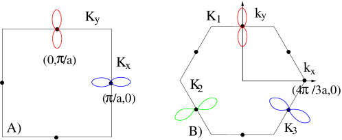
Figure 2: The $p$-orbital band structure in the two dimensions: A) square and B) triangular lattices. In the square lattice, the band minima are located at $K_{x}=(\pi/a_{0},0)$ for the $p_{x}$-orbital band, and $K_{y}=(0,\pi/a_{0})$ for the $p_{y}$-orbital band, respectively. In the triangular lattice, the band minima are at three middle points of Brillouin zone edges as $K_{1}=(0,\frac{2\pi}{\sqrt{3}a})$ and $K_{2,3}=(\frac{\pi}{a},\pm\frac{\pi}{\sqrt{3}a})$. The corresponding orbital configurations at these three band minimal are polar-like and parallel to the momentum directions of $K_{1,2,3}$ respectively as depicted.

The $p$-orbital Hamiltonian within the tight-binding approximation can be written as

$$H_{0}=t_{\parallel}\sum_{\langle ij\rangle}[p^{\dagger}_{i,\hat{e}_{ij}}p_{j,\hat{e}_{ij}}+h.c.]-t_{\perp}\sum_{\langle ij\rangle}[p^{\dagger}_{i,\hat{f}_{ij}}p_{j,\hat{f}_{ij}}+h.c.],$$ (3)

where the unit vector $\hat{e}_{ij}$ is along the bond orientation between two neighboring sites $i$ and $j$ and $\hat{f}_{ij}=\hat{z}\times\hat{e}_{ij}$ is perpendicular to $\hat{e}_{ij}$. $p_{\hat{e}_{ij}}$ and $p_{\hat{f}_{ij}}$ are the projections of $p$-orbitals along (perpendicular to) the bond direction respectively as defined below

$$p_{\hat{e}_{ij}}=(p_{x}\hat{e}_{x}+p_{y}\hat{e}_{y})\cdot\hat{e}_{ij},\ \ \ p_{\hat{f}_{ij}}=(p_{x}\hat{e}_{x}+p_{y}\hat{e}_{y})\cdot\hat{f}_{ij}.$$ (4)

The $\sigma$-bonding $t_{\parallel}$ and the $\pi$-bonding $t_{\perp}$ describe the hoppings along and perpendicular to the bond direction as depicted in Fig. 1 C and D, respectively. The opposite signs of the $\sigma$ and $\pi$-bondings are due to the odd parity of $p$-orbitals. $t_{\perp}$ is usually much smaller than $t_{\parallel}$ in strong periodical potentials.

Eq. 3 exhibits degenerate band minima in both the square and triangular lattice[2, 3, 13]. In the square lattice, the Brillouin zone (BZ) is a square with the edge length of $\frac{\pi}{a_{0}}$ where $a_{0}$ is the length between the nearest neighbors. The spectra read $\epsilon_{p_{x}}=t_{\parallel}\cos k_{x}-t_{\perp}\cos k_{y}$ and $\epsilon_{p_{y}}=-t_{\perp}\cos k_{x}+t_{\parallel}\cos k_{y}$. As depicted in Fig. 2. A, the band minima are located at $\vec{K}_{px}=(\frac{\pi}{a_{0}},0)$ for the $p_{x}$-band and $\vec{K}_{py}=(0,\frac{\pi}{a_{0}})$ for the $p_{y}$-band, respectively.

In the triangular lattice, we set the $\pi$-bonding to zero which does not change the qualitative band structures. We take unit vectors from one site to its six neighbors as $\pm\hat{e}_{1,2,3}$ with $\hat{e}_{1}=\hat{e}_{x}$, $\hat{e}_{2,3}=-\frac{1}{2}\hat{e}_{x}\pm\frac{\sqrt{3}}{2}\hat{e}_{y}$. The Brillouin zone takes the shape of a regular hexagon with the edge length $4\pi/(3a)$. The energy spectrum of $H_{0}$ is

$$E(k)=t_{\parallel}\Big{\{}f_{\vec{k}}\mp\sqrt{f^{2}_{\vec{k}}-3g_{\vec{k}}}\Big{\}},$$ (5)

with

$$f_{\vec{k}}=\sum_{i=1}^{3}\cos(\vec{k}\cdot\hat{e}_{i}),\ \ \ g_{\vec{k}}=\sum_{3\geq i>j\geq 1}\cos(\vec{k}\cdot\hat{e}_{i})\cos(\vec{k}\cdot\hat{e}_{j}).$$ (6)

The spectrum contains three degenerate minima located at the three non-equivalent middle points of the edges as $K_{1}=(0,\frac{2\pi}{\sqrt{3}a}),K_{2,3}=(\pm\frac{\pi}{a},\frac{\pi}{\sqrt{3}a})$, The factor $e^{i\vec{K}_{1}\cdot\vec{r}}$ takes the value of $\pm 1$ uniformly in each horizontal row but alternating in adjacent rows. If the above pattern is rotated at angles of $\pm\frac{2\pi}{3}$, then we arrive at the patterns of $e^{i\vec{K}_{2,3}\cdot\vec{r}}$. Each eigenvector is a 2-component superposition vector of $p_{x}$ and $p_{y}$ orbitals. The eigenvectors at energy minima are $\psi_{K_{1}}=e^{i\vec{K}_{1}\cdot\vec{r}}|p_{y}\rangle$. $\psi_{K_{2,3}}$ can be obtained by rotating $\psi_{1}$ at angles of $\pm\frac{2\pi}{3}$ respectively as depicted in Fig. 2 B.

2.3 Weak coupling analysis – BEC at nonzero momenta

If there were no interactions, any linear superposition of the above band minima would be a valid condensate wavefunctions. However, interactions will select a particular type combination which exhibits TR symmetry breaking and agrees with the above picture of “orbital Hund’s rule”.

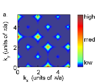
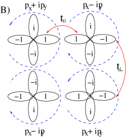
Figure 3: A) The time-of-flight spectra of the $p$-orbital Bose condensation in the square lattice. The coherence peaks occurs at $(m\frac{\pi}{a_{0}},(n+\frac{1}{2})\frac{\pi}{a_{0}})$, and $((m+\frac{1}{2})\frac{\pi}{a_{0}},n\frac{\pi}{a_{0}})$. B) The staggered ordering of OAM moments in the square lattice with the phase pattern on each site. Each of the $\sigma$ and $\pi$-bonds achieves phase coherence. From Liu and Wu, Ref 2.

2.3.1 The square lattice – the staggered ordering of OAM moments

In the square lattice, we take the condensate wavefunction as $\Psi_{sq}(\vec{r})=c_{1}\psi_{p_{x}}(K_{p_{x}})+c_{2}\psi_{p_{y}}(K_{p_{y}})$ under the constraint of $|c_{1}|^{2}+|c_{2}|^{2}=1$. Any choice of $c_{1,2}$ minimizes the kinetic energy. However, the interaction $U$-terms break the degeneracy. The degenerate perturbation theory shows that the ground state values of $c_{1,2}$ take $c_{1}=1,c_{2}=i$ or its equivalent TR partner of $c_{1}=1,c_{2}=-i$. The mean field condensate can be described as

$$\frac{1}{\sqrt{N_{0}!}}\Big{\{}\frac{1}{\sqrt{2}}(\psi^{\dagger}_{K_{p_{x}}}+i\psi^{\dagger}_{K_{p_{y}}})\Big{\}}^{N_{0}}|0\rangle,$$ (7)

where $N_{0}$ is the particle number in the condensate.

For better insight, we transform the above momentum space condensate to the real space. The orbital configuration on each site reads

$$e^{i\phi_{\vec{r}}}(|p_{x}\rangle+i\sigma_{\vec{r}}|p_{y}\rangle),$$ (8)

where the $U(1)$ phase $e^{i\phi_{\vec{r}}}$ is specified at the right lobe of the $p$-orbital. The Ising variable $\sigma_{\vec{r}}=\pm 1$ denotes the direction of the OAM, and is represented by the anti-clockwise (clockwise) arrow on each site in Fig. 3 B. Each site exhibits a nonzero OAM moment and breaks TR symmetry. The condensate wavefunction of Eq. 7 describes the staggered ordering of $\sigma_{\vec{r}}$. We check that the phase difference is zero along each bond, and thus no inter-site bond current exists.

The condensate described in Eq. 7 breaks both TR reversal and translational symmetries, and thus corresponds to a BEC at non-zero momenta. This feature should exhibit itself in the time-of-flight experiments which have been widely used to probe the momentum distribution of cold atoms. The coherence peaks of Eq. 7 are not located at integer values of the reciprocal lattice vectors but at $(m\frac{\pi}{a_{0}},(n+\frac{1}{2})\frac{\pi}{a_{0}})$, and $((m+\frac{1}{2})\frac{\pi}{a_{0}},n\frac{\pi}{a_{0}})$ as depicted in Fig. 3 A. Furthermore unlike the $s$-orbital condensate the $p$-wave Wannier function superposes a non-trivial profile on the height of density peaks. As a result, the highest peaks are shifted from the origin—a standard for the $s$-wave peak—to the reciprocal lattice vectors whose magnitude is around $1/l$ where $l$ is the characteristic length scale of the harmonic potential of each optical site. A detailed calculation of form factors is given in Ref. [2].

2.3.2 Excitations – gapless phonons and gapped orbital modes

The elementary excitations in $p$-orbital BECs consist of both the gapless phonon mode and the gapped orbital mode. The former corresponds to the Goldstone mode related to the $U(1)$ symmetry breaking, and the latter corresponds to the flipping of the direction of OAM moments. In the following, we will take the 2D square lattice as an example.

We assume the condensate as $\frac{1}{\sqrt{2}}[p^{\dagger}_{x}(Q_{x})+ip^{\dagger}_{y}(Q_{y})]$ with $Q_{x}=(\pi,0)$ and $Q_{y}=(0,\pi)$. The boson operators take the expectation values as

$$\langle|p_{x}(\vec{r})|\rangle=(-1)^{r_{x}}\phi,\ \ \ \langle|p_{y}(\vec{r})|\rangle=i(-1)^{r_{y}}\phi.$$ (9)

From minimizing the onsite part of the free energy respect to the condensate order parameter $\phi$

$$F=-\mu n+\frac{U}{2}(n^{2}-\frac{1}{3}L_{z}^{2}),$$ (10)

we have $\mu=\frac{4U}{3}|\phi|^{2}$ respect to the band minima. The fluctuation around the expectation value is defined as

$$p_{x}(\vec{r})=\langle|p_{x}(\vec{r})\rangle+\delta p_{x},\ \ \ p_{y}(\vec{r})=\langle|p_{y}(\vec{r})\rangle+\delta p_{y}.$$ (11)

Then the interaction terms in Eq. 2 are expanded as

$$H_{int} = \frac{4}{3}|\phi|^{4}+[\delta p^{\dagger}_{x}\delta p_{x}+\delta p^{\dagger}_{y}\delta p_{y}]\frac{8}{3}|\phi|^{2}+\frac{1}{3}\phi^{*,2}[\delta p_{x}\delta p_{x}-\delta p_{y}\delta p_{y}]$$ (12)

$$+ \frac{1}{3}\phi^{2}[\delta p_{x}^{\dagger}\delta p_{x}^{\dagger}-\delta p_{y}^{\dagger}\delta p_{y}^{\dagger}]+\frac{2i}{3}(-)^{r_{x}+r_{y}}[\phi^{2}\delta p_{x}^{\dagger}\delta p_{y}^{\dagger}-\phi^{*,2}\delta p_{x}\delta p_{y}].$$

Combined with the free part, we arrive the mean field Hamiltonian as

$$H_{MF}=\sum_{\vec{k},a,b}^{\prime}\Psi^{\dagger}(\vec{k})_{a}M_{ab}(\vec{k})\Psi_{b}(\vec{k})$$ (13)

where $\Psi^{\dagger}(\vec{k})=[p^{\dagger}_{x}(\vec{k}),p^{\dagger}_{y}(\vec{k}+\vec{Q}),p_{x}(-\vec{k}),p_{y}(-\vec{k}-\vec{Q})]$, $\vec{Q}=(\pi,\pi)=\vec{Q}_{x}-\vec{Q}_{y}$, and the summation is only over half of the Brillouin zone. The matrix kernel reads

$$M(\vec{k})=\left(\begin{array}[]{cccc}\epsilon_{x}(\vec{k})+\frac{4U}{3}|\phi|^{2}&0&\frac{2U}{3}\phi^{2}&i\frac{2U}{3}\phi^{2}\\ 0&\epsilon_{y}(\vec{k}+\vec{Q})+\frac{4U}{3}|\phi|^{2}&i\frac{2U}{3}\phi^{2}&\frac{2U}{3}\phi^{2}\\ \frac{2}{3}U\phi^{*,2}&-\frac{2i}{3}U\phi^{*,2}&\epsilon_{x}(\vec{k})+\frac{4U}{3}|\phi|^{2}&0\\ -\frac{2i}{3}U\phi^{*,2}&\frac{2}{3}U\phi^{*,2}&0&\epsilon_{y}(\vec{k}+\vec{Q})+\frac{4U}{3}|\phi|^{2}\end{array}\right).$$ (18)

The spectra are reduced to generalized eigenvalue problem of

$$X^{-1}\big{\{}\mbox{diag}(1,1,-1,-1)~{}M(\vec{k})\big{\}}X=\mbox{diag}(E_{1},E_{2},-E_{3},-E_{4}),$$ (19)

where $E_{1,2,3,4}(\vec{k})$ are excitation eigenvalues, and $X$ contains the eigenvectors.

Let us consider the excitation close to the condensation wavevector $\vec{k}=\vec{Q}_{x}+\vec{q}$, and then $\vec{k}+\vec{Q}=\vec{Q}_{y}+\vec{q}$. At small value of $\vec{q}$, we obtain the excitation spectra as

$$E_{1,3}(\vec{k}) = \sqrt{\bar{\epsilon}(\vec{q})(\bar{\epsilon}(\vec{q})+\frac{8}{3}U|\phi|^{2})},\ \ \ E_{2,4}(\vec{k})=\bar{\epsilon}(\vec{q})+\frac{4}{3}U|\phi|^{2}.$$ (20)

where $\bar{\epsilon}(\vec{q})=\frac{1}{2}[\epsilon_{x}(\vec{Q}_{x}+\vec{q})+\epsilon_{y}(\vec{Q}_{y}+\vec{q})-\epsilon_{x}(\vec{Q}_{x})-\epsilon_{y}(\vec{Q}_{y})]\approx\frac{t_{\parallel}+t_{\perp}}{2}(q_{x}^{2}+q_{y}^{2})$. Clearly, the gapless mode with the linear dispersion relation describes the superfluid phase fluctuations; the gapped mode describes the orbital excitations corresponding to the flipping of orbital angular momenta.

2.3.3 The triangular lattice – the stripe ordering of OAM moments

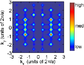
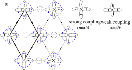
Figure 4: A) The time-of-flight spectra of the $p$-orbital boson condensation in the triangular lattice. The coherence peaks occurs at B) The stripe ordering of OAM moments in the triangular lattice. From Wu et al. Ref. 3.

In the triangular lattice, the OAM moments instead form a stripe ordering, i.e., the OAM moments along one row polarizes along the $z$-axis and those along the neighouring rows polarizes with the opposite direction. This can be intuitively understood as follows. In the superfluid state, the OAM moments behave like vortices whose interactions are long range. The above stripe configuration of positive and negative vortices is the optimal configuration to minimize the globe vorticity.

Let us first examine the weak coupling limit. Again we write a general form for condensation wavefunction as a linear superposition of the three band minima

$$\Psi_{c}(\vec{r})=\frac{1}{\sqrt{N}}(c_{1}\psi_{K_{1}}+c_{2}\psi_{K_{2}}+c_{3}\psi_{K_{3}}),$$ (21)

where $K_{1,2,3}$ are the locations of band minima defined in Sect. 2.2. Without loss of generality, we set $c_{1}=1$, and define $x=(c_{2}+c_{3})/2$, $y=(c_{2}-c_{3})/2$ and $x=x_{1}+ix_{2}$ and $y=y_{1}+iy_{2}$, then the normalization factor $N=\sqrt{1+2(x_{1}^{2}+y_{1}^{2}+x_{2}^{2}+y_{2}^{2})}$. The interaction energy persite is calculated as

$$E_{int} = \frac{1}{N^{2}}\big{\{}(x_{1}^{2}+x_{2}^{2}-y_{1}^{2}-y_{2}^{2})^{2}+8x_{1}^{2}+8y_{1}^{2}\big{\}}+1$$ (22)

$$- \frac{1}{N^{2}}\big{\{}4(x_{1}y_{2}-x_{2}y_{1})^{2}+2x_{2}^{2}+2y_{2}^{2}\big{\}}.$$

The terms in the first line are from the density-density interaction which can be minimized by setting $x_{1}=y_{1}=0$ and $x_{2}=\pm y_{2}$. This means only one of $c_{2,3}$ is nonzero and purely imaginary. In this case, the particle number on each site is uniform. The terms in the second line can also be minimized at this condition with a further requirement of $x_{2}=\pm y_{2}=\pm\frac{1}{2}$. If we take $c_{2}$ nonzero, then $c_{2}=\pm i$. Thus the mean field condensate can be expressed as $\frac{1}{\sqrt{N_{0}!}}\Big{\{}\frac{1}{\sqrt{2}}(\psi^{\dagger}_{K_{2}}+i\psi^{\dagger}_{K_{3}})\Big{\}}^{N_{0}}|0\rangle$ with $|0\rangle$ the vacuum state and $N_{0}$ the particle number in the condensate. This state breaks the $U(1)$ gauge symmetry, as well as TR and lattice rotation symmetries, thus the ground state manifold is $U(1)\otimes Z_{2}\otimes Z_{3}$. This state also breaks lattice translation symmetry, which is, however, equivalent to suitable combinations of $U(1)$ and lattice rotation operations.

Again we transform the above momentum space condensate to the real space, whose orbital configuration takes

$$e^{i\phi_{\vec{r}}}(\cos\alpha|p_{x}\rangle+i\sigma_{\vec{r}}\sin\alpha|p_{y}\rangle)$$ (23)

with $\alpha=\frac{\pi}{6}$ as $U/t\rightarrow 0$. The general configuration of $\alpha$ is depicted in Fig. 4 B for later convenience. At $U/t\rightarrow 0$, $p_{x,y}$ are not equally populated, and the moment per particle is $\frac{\sqrt{3}}{2}\hbar$. This does not fully optimize $H_{int}$ which requires $L_{z,\vec{r}}=\pm\hbar$. However, it fully optimizes $H_{0}$ which dominates over $H_{int}$ in the weak coupling limit. We check that the phase difference is zero along each bond, and thus no inter-site bond current exists.

Interestingly, as depicted in Fig. 4 B, OAM moments form a stripe order along each horizontal row. This stripe ordering in the weak coupling limit is robust at small values of the $\pi$-bonding $t_{\perp}$ because it does not change the location of the band minima and the corresponding eigenfunctions of $\Psi_{K_{1,2,3}}$ at all.

The driving force for this stripe formation in the SF regime is the kinetic energy, i.e., the phase coherence between bosons in each site. By contrast, the stripe formation in high T_c cuprates is driven by the competition between long range repulsion and the short range attraction in the interaction terms [33].

This stripe phase should manifest itself in the time of flight (TOF) signal as depicted in Fig. 4 A. In the superfluid state, we assume the stripe ordering wavevector $K_{1}$, and the corresponding condensation wavevectors at $K_{2,3}$. As a result, the TOF density peak position after a fight time of $t$ is shifted from the reciprocal lattice vectors $\vec{G}$ as follows

$$\langle n(\vec{r})\rangle_{t} \propto \sum_{\vec{G}}\Big{\{}|\phi_{2}(\alpha,\vec{k})|^{2}\delta^{2}(\vec{k}-\vec{K}_{2}-\vec{G})+|\phi_{3}(\alpha,\vec{k})|^{2}\delta^{2}(\vec{k}-\vec{K}_{3}-\vec{G})\Big{\}},$$ (24)

where $\vec{k}=m\vec{r}/(\hbar t)$; $\phi_{2,3}(\alpha,\vec{k})$ is the Fourier transform of the Wannier $p$-orbital wavefunction $|\phi_{2,3}(\alpha)\rangle$, and $\vec{G}=\frac{2\pi}{a}[m,(-m+2n)/\sqrt{3}]$ with $m,n$ integers. Thus Bragg peaks should occur at $\frac{2\pi}{a}[m\pm\frac{1}{2},\frac{1}{\sqrt{3}}(-m+2n+\frac{1}{2})]$. Due to the form factors of the $p$-wave Wannier orbit wavefunction $|\phi_{2,3}(\alpha,\vec{k})|^{2}$, the locations of the highest peaks is not located at the origin but around $|k|\approx 1/l_{x,y}$. Due to the breaking of lattice rotation symmetry, the pattern of Bragg peaks can be rotated at angles of $\pm\frac{2\pi}{3}$.

2.4 Strong coupling analysis – the lattice gauge theory formalism

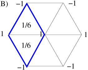
Figure 5: A) Strong coupling analysis for the inter-site coupling between OAM moments on neighboring sites. The OAM moments are described by Ising variables $\sigma_{ij}$. $\theta_{i}$ and $\theta_{j}$ are the azimuthal angles of the bonds relative the $x$-axis. B) The stripe ordering of OAM moments in the triangular lattice. The smallest unit is rhombic with the total vorticity of $1/3$.

In this subsection, the ordering of the OAM moments in the strong coupling superfluid regime is examined. We will employ the lattice gauge theory formalism developed by Moore and Lee in Ref. [34] in the context of the $p+ip$ Josephson junction array systems.

In the superfluid regime, each site $i$ is denoted by a $U(1)$ variable $\phi_{i}$ which denotes the superfluid phase along the $x$-direction, and by an Ising variable $\sigma_{z,i}=\pm 1$ for the direction of the OAM moment as depicted in Fig. 5. Along a general direction of the azimuthal angle $\theta$, the superfluid phase is $\phi_{i}+\sigma_{z,i}\theta$. The intersite $\sigma$ and $\pi$-bonding become the intersite Josephson coupling as

$$H_{ij}=-nt_{\parallel}\cos(\phi_{i}-\phi_{j}-A_{\parallel}(i,j))-nt_{\perp}\cos(\phi_{i}-\phi_{j}-A_{\perp}(i,j)),$$ (25)

where $n$ is the average particle number per site. The phase differences in Eq. 25 takes into account the geometric orientation of the bond $\langle ij\rangle$ as captured by the gauge fields $A_{\parallel}$ and $A_{\perp}$ with the definition that $A_{\parallel}=\sigma_{z,i}\theta_{i}-\sigma_{z,j}\theta_{j}$, $A_{\perp}=\sigma_{z,i}(\theta_{i}+\frac{\pi}{2})-\sigma_{z,j}(\theta_{j}-\frac{\pi}{2})=A_{\parallel}+\frac{\pi}{2}(\sigma_{z,i}+\sigma_{z,j})$, and $\theta_{j}=\theta_{i}+\pi$ are the azimuth angles relative to the $x$-axis defined in Fig. 5.

Let us first consider the case of $t_{\perp}\neq 0$ and write down an effective Hamiltonian for the Ising variables $\sigma_{z}$. In order to minimize both the Josephson couplings of the $\sigma$ and $\pi$-bonds, we need $\sigma_{i}=-\sigma_{j}$ and thus $A_{\parallel,ij}=A_{\perp,ij}$. Otherwise, if $\sigma_{i}=\sigma_{j}$, then $A_{\parallel,ij}=A_{\perp,ij}+\pi$. This costs an energy of $2t_{\perp}$, and leads to an effective antiferro-orbital interaction between the Ising variables as

$$H_{eff}=nt_{\perp}\sum_{ij}\sigma_{z,i}\sigma_{z,j}.$$ (26)

Thus the antiferro-orbital ordering of OAM moments in the square lattice remains valid in the strong coupling limit at non-vanishing $t_{\perp}$, which enforces that both the $\sigma$ and $\pi$-bonds achieve phase coherence as depicted in Fig. 3. B.

On the other hand, in the limit of a vanishing $t_{\perp}$, the leading order effect involves multiple site interaction around a plaquette. We follow the method described in Ref. [34], and perform the duality transformation for the $U(1)$ phase variables $\phi$ under the background of the geometric gauge potential $A_{\parallel}$. We separate the contributions from the phonon part and the vortex part as

$$Z = Z_{ph}\sum_{m}^{\prime}\exp\Big{\{}-\frac{\pi^{2}nt_{\parallel}}{2}\sum_{x}(m(x)-\Phi_{x})^{2}$$ (27)

$$+ \pi nt_{\parallel}\sum_{x\neq x^{\prime}}(m(x)-\Phi_{x})\log\frac{|x-x^{\prime}|}{a}(m(x^{\prime})-\Phi_{x}^{\prime})\Big{\}},$$

where $Z_{ph}$ is the phonon contribution in the vortex-free configuration; $x$ marks the dual lattice site (or the plaquette index in the original lattice); $m$ is the vortex charge; $\Phi_{x}$ is the external flux through the plaquette defined as

$$\Phi_{x}=\frac{1}{2\pi}\sum_{ij}A_{\parallel,ij}.$$ (28)

In the square lattice, the geometric gauge flux around each plaquette $x$ is calculated as

$$\Phi_{x}=-\frac{1}{4}(\sigma_{i}+\sigma_{i+e_{x}}+\sigma_{i+e_{x}+e_{y}}+\sigma_{i+e_{y}}).$$ (29)

If $\Phi_{x}$ is integer-valued, it can be absorbed by shifting the zero of the vortex charge as $m^{\prime}(x)=m(x)-\Phi_{x}$ which remains integer-valued, thus there is no cost for energy. The feature can be captured by the effective Hamiltonian in Ref. [34] as

$$H_{eff}=-K\sum_{ijkl}\sigma_{i}\sigma_{i}\sigma_{k}\sigma_{l},$$ (30)

where $i,j,k,l$ are four sites around a plaquette centered at $x$; $K\approx nt_{\parallel}$ is the energy scale of the $\sigma$-bonding. This model has a sub-extensive $Z_{2}$ symmetry investigated in Ref. [34], i.e., flipping the sign of $\sigma_{z}$ along each row or column leave Eq. 30 invariant. Thus it cannot develop the ordering of OAM at any finite temperature. Let us come back to the superfluid sector $\phi$, its most relevant topological defect is the half-quantum vortices because $\Phi_{x}$ can take the values of $\pm\frac{1}{2}$. The Kosterlitz-Thouless transition is associated with the unbinding of half-quantum vortices. As a result, the low temperature phase is the quasi-long range ordering of pairing of bosons [34].

Next we move to the strong coupling theory in the triangular lattice. We start from the limit of $t_{\perp}=0$. The geometrical gauge flux becomes

$$\Phi_{x}=-\frac{1}{6}(\sigma_{1}+\sigma_{2}+\sigma_{3}),$$ (31)

where $1,2,3$ are three sites around a triangular plaquette. There is no way to form an integer flux. The smallest vorticity per plaquette is $\pm\frac{1}{6}$ which corresponds to either two $+1$’s and one $-1$, or two $-1$’s and one $+1$ to minimize the vortex core energy. In such a dense vortex configuration, Eq. 27 rigorously speaking does not apply because its validity relies on the assumption of small vortex fugacity. However, the structure of interactions among vortices still implies that vortices form a regular lattice with alternating positive and negative vorticity. The dual lattice (the center of the triangular plaquette) is the bipartite honeycomb lattice. It is tempting to assign $\pm\frac{1}{6}$ alternatively to each plaquette, but actually it is not possible due to the following reason. Consider a plaquette with vorticity $+\frac{1}{6}$, thus its three vertices are with two $+1$’s and one $-1$. The neighboring plaquette sharing the edge with two $+1$’s must have the same vorticity, and merges with the former one to form a rhombic plaquette with vorticity $\frac{1}{3}$ as depicted in Fig. 5 B. Thus the ground state should exhibit a staggered pattern of rhombic plaquette with vorticity of $\pm\frac{1}{3}$. This arrangement precisely corresponds to the stripe order of the Ising variables. This configuration breaks both the lattice rotational and translational symmetries, which is six-fold degenerate. If we turn on the small $t_{\perp}$ term, it results in an antiferromagnetic Ising coupling with nearest bonds, the stripe configuration also satisfies its ground state requirement. Thus we believe that $t_{\perp}$ term does not change the stripe configuration in the strong coupling limit either.

Having established the stripe order for the OAM moments, it is straightforward to further optimize the $U(1)$ phase variable $\phi$. The result is depicted in Fig. 4 B with $\phi$ marked on the right lobe of the $p_{x}\pm ip_{y}$ orbit. Each horizontal bond has perfect phase match, while each of tilted bond has a phase difference of $\frac{\pi}{12}$. Thus around each rhombic plaquette, the phase winding is $\frac{\pi}{12}\times 4=\frac{\pi}{3}$ and gives rise to the Josephson supercurrent along the bonds as

$$j=\frac{t_{\parallel}n}{2}\sin\Delta\theta,$$ (32)

with $\Delta\theta=\frac{\pi}{6}$ and the directions specified by arrows in Fig. 4 B. In other words, in addition to the stripe order of the Ising variables which corresponds to the onsite OAM moments, there exists a staggered plaquette bond current order. This feature does not appear in the square lattice [2]. The orbital plaquette current ordering has been studied in the strongly correlated electron systems, such as the circulating orbital current phase [35] and the d-density wave states in the high T_c compounds [36]. It is amazing that in spite of very different microscopic mechanism and energy scales, the two completely different systems exhibit a similar phenomenology.

2.5 Intermediate coupling regime in the triangular lattice – self-consistent mean field analysis

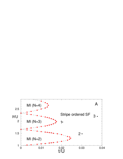
Figure 6: A) Phase diagram based on the GMF theory in the $2\times 2$ unit cell (see Fig. 4 B). Large scale Gutzwiller mean field calculations in a $30\times 30$ lattice are performed to confirm the stripe ordered superfluid (SF) phase at points 1, 2 and 3 with $(t/U,\mu/U)=(0.02,2),(0.03,1.5)$ and $(0.038,2.2)$, respectively. B) The flux $\Phi$ around a rhombic plaquette v.s. $t/(nU)$. It decays from $\frac{1}{3}$ in the strong coupling limit to $0$ in the non-interaction limit. The solid line is the Gutzwiller result at $n=3$, while the dashed line is based on the energy function Eq. 35 of the trial condensate. From Wu et. al, Ref. 3.

We have shown that in the triangular lattice the stripe ordering of the OAM moments exist in both weak and strong coupling superfluid states. The orbital configurations are slightly different: the orbital mixing angle $\alpha$ defined in Eq. 23 equals to $\frac{\pi}{6}$ in the weak coupling limit, while it equals to $\frac{\pi}{4}$ in the strong coupling limit. This arises from the competition between the kinetic energy and the onsite Hund’s rule. Below we will see that as $U/t_{\parallel}$ goes from small to large, the stripe ordering remains the same with a smooth evolution of $\alpha$ from $\frac{\pi}{6}$ to $\frac{\pi}{4}$ as depicted in Fig. 4 B.

We use a Gutzwiller type mean field theory for a $30\times 30$ lattice under the periodic boundary condition. We explicitly checked for three sets of parameters $(t_{\parallel}/U,\mu/U)$ marked as points of $1,2$ and $3$ in Fig. 6 B. The stripe-ordered ground state with a $2\times 2$ unit cell depicted in Fig. 4 A is found stable against small random perturbations in all the three cases. Then we further apply the Gutzwiller type theory assuming a $2\times 2$ unit cell and obtain the phase diagram depicted in Fig. 6 A which includes both the stripe ordered superfluid phase and Mott-insulating phases.

In order to gain a better understanding of the numerical results, we write the trial condensate with the $p$-orbital configuration on each site as

$$e^{i\phi_{\vec{r}}}(\cos\alpha|p_{x}\rangle+i\sigma_{\vec{r}}\sin\alpha|p_{y}\rangle).$$ (33)

We have checked that the optimal pattern for the $U(1)$ phase $\phi_{\vec{r}}$ does not depend on the orbital mixing angle of $\alpha$, and it also remains the same for all the coupling strength. The phase mismatch $\Delta\theta$ defined in Eq. 32 on the tilted bonds for a general orbital mixing angle $\alpha$ can be calculated through simple algebra as

$$\Delta\theta=2\gamma-\pi/2,\ \ \ \mbox{with}~{}~{}\tan\gamma={\sqrt{3}}\tan\alpha,$$ (34)

and the corresponding Josephson current is $j=nt\sin\Delta\theta$. The value of $\alpha$ is determined by the minimization of the energy per particle of the trial condensate as

$${\cal E}(\alpha)=-t[1+2\sin(2\alpha+\frac{\pi}{6})]-\frac{nU}{6}\sin^{2}2\alpha+\frac{nU}{3},$$ (35)

where the first term is the contribution from the kinetic energy which requires phase coherence, and the second term is the interaction contribution reflecting the Hund’s rule physics. In the strong and weak coupling limits, the energy minimum is located at $\alpha=\frac{\pi}{4}$ and $\frac{\pi}{6}$, respectively. The corresponding fluxes in each rhombic plaquette $\Phi=4\Delta\theta/(2\pi)=0$ and $\pm\frac{1}{3}$ respectively, which agree with the previous analyses. In the intermediate coupling regime, we present both results of $\Phi$ at $n=3$ based on the Gutzwiller mean field theory and those of Eq. (35) in Fig. 6B. They agree with each other very well, and confirm the validity of the trial condensate wavefunction. Moreover, in the momentum space, the trial condensate for a general $\alpha$ can be expressed as $\frac{1}{\sqrt{N_{0}!}}\Big{\{}\frac{1}{\sqrt{2}}(\psi^{\prime\dagger}_{K_{2}}+i\psi^{\prime\dagger}_{K_{3}})\Big{\}}^{N_{0}}|0\rangle,$ where $\psi^{\prime}_{K_{2,3}}(\vec{r})=e^{i\vec{K}_{2,3}\cdot\vec{r}}|\phi_{2,3}(\alpha)\rangle$ with $|\phi_{2,3}(\alpha)\rangle=-\cos\alpha|p_{x}\rangle\mp\sin\alpha|p_{y}\rangle$ respectively.

2.6 Orbital angular momentum ordering in the Mott-insulating states

So far, we have only discussed the orbital ordering in the superfluid states. Since the OAM moment is a different degree of freedom from the superfluid phase, we expect that its ordering can survive even inside the Mott-insulating phases. In this subsection, we continue to study the exchange physics of orbital bosons and the related ordering of OAM moments in the absence of the superfluidity order. For simplicity, we will use the triangular lattice as an example.

We consider the Mott-insulating phases with $n$ spinless bosons per-site and two degenerate orbitals of $p_{x}$ and $p_{y}$. We define the TR doublets of all the particles in the states of $p_{x}\pm ip_{y}$ as the eigenstates of the Ising operator $\sigma_{z}$ with the eigenvalues of $\pm 1$. The Ising part of the effective exchange Hamilton occurs at the level of the second order perturbation theory, while the Ising variable flipping process occurs at the $2n$-th order perturbation theory. We consider the large-$n$ case in which the system is deeply inside the Ising anisotropy class, and no orbital-flip process occurs at the leading order. In the following, we will study the physics of the $2,3,4$-site exchange processes.

2.6.1 The two-site exchange

Let us consider the virtual hopping processes in the Mott-insulating states along the bond depicted in Fig. 5 A. Both the $\sigma$-bonding $t_{\parallel}$ and $\pi$-bonding $t_{\perp}$ are kept. With the definition of $p^{\dagger}_{\pm}=\frac{1}{\sqrt{2}}(p_{x}^{\dagger}\pm ip_{y}^{\dagger}),$ we can express the hopping as

$$H_{t} = -\frac{1}{2}\sum_{\sigma\sigma^{\prime}}\Big{\{}t_{\parallel}p^{\dagger}_{\sigma}(j)p_{\sigma^{\prime}}(i)e^{-i(\sigma\theta_{j}-\sigma^{\prime}\theta_{i})}+t_{\perp}p^{\dagger}_{\sigma}(j)p_{\sigma^{\prime}}(i)e^{-i(\sigma-\sigma^{\prime})(\theta_{i}+\frac{\pi}{2})}+h.c.\Big{\}}$$ (36)

$$= \frac{t_{\parallel}-t_{\perp}}{2}\sum_{\sigma}\big{\{}p^{\dagger}_{j,\sigma}p_{i\sigma}+h.c.\big{\}}+\frac{t_{\parallel}+t_{\perp}}{2}\sum_{\sigma}\big{\{}p^{\dagger}_{j,\sigma}p_{i,-\sigma}e^{-2i\sigma\theta_{i}}+h.c.\big{\}},$$

where the definition of angles $\theta_{i},\theta_{j}$ follows the convention depicted in Fig. 5 A.

We calculate the energy shifts in both the ferro-orbital configurations ($\sigma_{i}=\sigma_{j}$) and the antiferro-orbital configurations ( $\sigma_{i}=\bar{\sigma}_{j}$) within the second order perturbation theory. The energy difference between these two configurations is

$$\Delta E_{FO} = -\frac{2n(n+1)[(t_{\parallel}-t_{\perp})/2]^{2}}{\Delta E_{1}}-\frac{2n[(t_{\parallel}+t_{\perp})/2]^{2}}{\Delta E_{2}}$$

$$\Delta E_{AFO} = -\frac{2n(n+1)[(t_{\parallel}+t_{\perp})/2]^{2}}{\Delta E_{1}}-\frac{2n[(t_{\parallel}-t_{\perp})/2]^{2}}{\Delta E_{2}},$$ (37)

where $\Delta E_{1}=\frac{2}{3}U$ and $\Delta E_{2}=\frac{2}{3}U(n+1)$. The antiferro-orbital configuration has lower energy, which arises from the fact that the orbital-flip process has a larger amplitude than that of the orbital non-flip process described in Eq. 36. This is because that the $\sigma$-bonding and $\pi$-bonding amplitudes have a $\pi$-phase shift. The Ising coupling $J_{AFO}$ reads

$$H=J_{AFO}\sum_{ij}\sigma_{z}(i)\sigma_{z}(j)$$ (38)

where $J_{AFO}\approx\frac{2n^{2}t_{\perp}t_{\parallel}}{3U}$ with only the leading order contribution kept. If $t_{\perp}$ is set to zero, $J_{AFO}$ varnishes. This is clear from the fact that we can flip the sign of the $p$-orbit component perpendicular to the bond direction. This operation changes the value of $\sigma_{z}$, but has no effect on the energy. In this case, we need to further study the multi-site virtual hopping processes.

2.6.2 The three-site ring exchange

The $\sigma$-bonding term by itself gives non-zero ring exchange terms for the multi-site processes, thus we neglect the contribution from the $\pi$-bonding part. In the following, we only keep the leading order virtual process proportional to $(nt_{\parallel})^{3}/U^{2}$.

We consider a triangular plaquette with three sites $(i,j,k)$ each of which is denoted by the particle number and the Ising variables as $(n,\sigma_{z,i}),(n,\sigma_{z,j}),(n,\sigma_{z,k})$, respectively. There are 12 different ring-hopping processes whose contribution is at the order of $(nt_{\parallel})^{3}/U^{2}$. We enumerate 4 of them explicitly as

$$(n,\sigma_{z,i})(n,\sigma_{z,j})(n,\sigma_{z,k})\rightarrow(n-1,\sigma_{z,i})(n+1,\sigma_{z,j})(n,\sigma_{z,k})$$ (39)

$$\rightarrow (n-1,\sigma_{z,i})(n,\sigma_{z,j})(n+1,\sigma_{z,k})\rightarrow(n,\sigma_{z,i})(n,\sigma_{z,j})(n,\sigma_{z,k})$$

$$(n,\sigma_{z,i})(n,\sigma_{z,j})(n,\sigma_{z,k})\rightarrow(n+1,\sigma_{z,i})(n-1,\sigma_{z,j})(n,\sigma_{z,k})$$

$$\rightarrow (n,\sigma_{z,i})(n-1,\sigma_{z,j})(n+1,\sigma_{z,k})\rightarrow(n,\sigma_{z,i})(n,\sigma_{z,j})(n,\sigma_{z,k})$$

$$(n,\sigma_{z,i})(n,\sigma_{z,j})(n,\sigma_{z,k})\rightarrow(n-1,\sigma_{z,i})(n+1,\sigma_{z,j})(n,\sigma_{z,k})$$

$$\rightarrow (n,\sigma_{z,i})(n+1,\sigma_{z,j})(n-1,\sigma_{z,k})\rightarrow(n,\sigma_{z,i})(n,\sigma_{z,j})(n,\sigma_{z,k})$$

$$(n,\sigma_{z,i})(n,\sigma_{z,j})(n,\sigma_{z,k})\rightarrow(n+1,\sigma_{z,i})(n-1,\sigma_{z,j})(n,\sigma_{z,k})$$

$$\rightarrow (n-1,\sigma_{z,i})(n,\sigma_{z,j})(n+1,\sigma_{z,k})\rightarrow(n,\sigma_{z,i})(n,\sigma_{z,j})(n,\sigma_{z,k}).$$

The other $8$ processes can be obtained by a cyclic permutation $i\rightarrow j\rightarrow k$. After sum over all these processes, the corresponding energy shift reads

$$\Delta E(\sigma_{i},\sigma_{j},\sigma_{k})\approx 6(\frac{-t_{\parallel}}{2})^{3}(n(n+1))^{3/2}\frac{e^{-i2\pi\Phi_{3}}+h.c.}{(\Delta E)^{2}} =-J_{3}\cos(2\pi\Phi_{3}),$$ (40)

where $J_{3}=\frac{3(nt)^{3}}{2(\Delta E)^{2}}$ and $\Delta E=\frac{2U}{3}$; $\Phi_{3}$ is defined as before in the superfluid case. Again for each plaquette, $\Phi_{3}$ takes the value of $\pm\frac{1}{6}$ which correspond to $\sigma_{z}$s taking the values of two $1$s and one $-1$ or two $-1$s and one $1$. Eq. 40 plays a similar role to vortex core energy in Eq. 27. Eq. 40 by itself has a huge ground state degeneracy because the requirement is the same as that of the antiferromagnetic Ising model. We need to add the four-site process to lift the degeneracy.

2.6.3 The four-site ring exchange

The four-site process mimics the interaction between two adjacent vortices. By the spirit of perturbation theory, the 4-particle process is further suppressed by a factor $\frac{nt_{\parallel}}{U}$, thus the interaction between vortices should be of short range. This makes sense in the Mott insulating state due to the condensation of vortices and the resulting screening effect.

Again we only consider the effect from the $\sigma$-bonding term, and only keep the leading order contribution at the level of $(nt)^{4}/U^{3}$. Similarly, we have 48 different virtual hopping processes. For a plaquette with vertices $(ijkl)$, the energy shift is

$$\Delta E(\sigma_{i},\sigma_{j},\sigma_{k},\sigma_{l})\approx-J_{4}\cos(2\pi\Phi_{4}),$$ (41)

where $J_{4}=\frac{5(nt)^{4}}{3(\Delta E)^{3}}$ . In the square lattice, $\Phi_{4}=(\sigma_{1}+\sigma_{2}+\sigma_{3}+\sigma_{4})/4$. If $t_{\perp}=0$, Eq. 41 is the leading order contribution, thus the effective Hamiltonian looks the same as that in the superfluid case but with a reduced coupling constant. If $t_{\perp}\neq 0$, then the two-site exchange of Eq. 38 results in the long range antiferro-orbital order.

In the triangular lattice, the $\Phi_{4}$ of the four-site plaquette $(ijkl)$ just equals the sum of the flux of the two triangular plaquettes. Since each triangular plaquette takes the flux value of $\pm\frac{1}{6}$, the rhombic four-site plaquette can only take the flux value of $0$, $\pm\frac{1}{3}$. The stripe ordering pattern gives the maximum number of the zero-flux four-site plaquettes, and thus is selected as the ground state. The stripe ordering appears at temperatures $T<J_{4}$ and disappears at $J_{3}>T>J_{4}$ in which the three-site exchange process dominates the physics.

3 Exotic condensation of bosons with spin-orbit coupling

In this section, we discuss another route for “complex-condensation” of bosons, i.e., spinful bosons with spin-orbit (SO) coupling. The proof of Feynman’s “no-node” theorem crucially relies on the fact that the kinetic energy of bosons only contains even power of momentum, thus SO coupling which linearly depends on momentum invalidates Feynman’s proof. In the following, we consider the simplest example of the two-component bosons with the Rashba-like SO coupling and investigate their condensate in the inhomogeneous harmonic traps. A related work on the BEC of two-component bosons has also been studied by Stanescu et al. in Ref. [11].

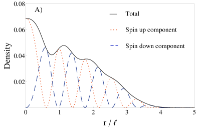
Figure 7: A)The radial density distribution of spin up and down components, and the total density distribution in the unit of $N_{0}$ at $\alpha=4$ and $\beta=40$. B) The spin density distribution along the $x$-axis which spirals in the $z$-$x$ plane at an approximate wavevector of $2k_{0}$, whose value at the origin is normalized to 1. The spin density in the whole plane exhibits the skyrmion configuration. From Wu et al. Ref. 5.

We consider bosons with two-components denoted as pseudospin up and down. The many-body Hamiltonian for interacting bosons is written as

$$H = \int d^{2}\vec{r}~{}~{}\psi^{\dagger}_{\alpha}\big{\{}-\frac{\hbar^{2}\nabla^{2}}{2M}-\mu+V_{ext}(\vec{r})\big{\}}\psi_{\alpha}$$ (42)

$$+ \hbar\lambda_{R}\psi^{\dagger}_{\alpha}(-i\nabla_{y}\sigma_{x}+i\nabla_{x}\sigma_{y})\psi_{\beta}+\frac{g}{2}\psi^{\dagger}_{\alpha}\psi^{\dagger}_{\beta}\psi_{\beta}\psi_{\alpha},~{}~{}~{}~{}~{}$$

where $\psi_{\alpha}$ is the boson operator; $\alpha$ refers to boson pseudospin $\uparrow$ and $\downarrow$; $V_{ext}$ is the external potential; $g$ describes the $s$-wave scattering interaction which is assumed to be spin-independent for simplicity; $\lambda_{R}$ is the Rashba SO coupling strength. Although Eq. 42 is of bosons, it satisfies a suitably defined TR symmetry like fermion systems as $T=i\sigma_{2}C$ with $T^{2}=-1$ where $C$ is the complex conjugate and $\sigma_{2}$ operates on the pseudospin doublet. In the homogeneous system, the single particle states are the helicity eigenstates of $\vec{\sigma}\cdot(\vec{k}\times\hat{z})$ with the dispersion relations of $\epsilon_{\pm}(\vec{k})=\frac{\hbar^{2}}{2M}(k\mp k_{0})^{2}$ where $k_{0}=\frac{M\lambda_{R}}{\hbar}$. The energy minima are located at the lower branch along a ring with radius $k_{0}$. The corresponding two-component wavefunction $\psi_{+}(\vec{k})$ with $|k|=k_{0}$ can be solved as $\psi_{+}^{T}(\vec{k})=\frac{1}{\sqrt{2}}(e^{-i\phi_{k}/2},ie^{i\phi_{k}/2})$, where $\phi_{k}$ is the azimuth angle of $\vec{k}$.

Instead of discussing the condensation in the homogeneous system in which frustrations occur due to the degeneracy of the single particle ground states, we consider a 2D system with an external harmonic trap with $V_{ex}(r)=\frac{1}{2}M\omega_{T}^{2}r^{2}$. We define the characteristic SO energy scale for the harmonic trap as $E_{so}=\hbar\lambda_{R}/l$ where $l=\sqrt{\hbar/(M\omega_{T})}$ is the length scale of the trap, and correspondingly a dimensionless parameter as $\alpha=E_{so}/(\hbar\omega_{T})=lk_{0}$. The characteristic interaction energy scale is defined as $E_{int}=gN_{0}/(\pi l^{2})$ where $N_{0}$ is the total particle number and the dimensionless parameter $\beta=E_{int}/(\hbar\omega_{T})$.

The Gross-Pitaevskii equation can be obtained as the saddle-point equation of Eq. 42 as

$$\Big{\{}-\frac{\hbar^{2}\vec{\nabla}^{2}}{2M} + \hbar\lambda_{R}(-i\nabla_{y}\sigma_{x,\alpha\beta}+i\nabla_{x}\sigma_{y,\alpha\beta})+g(\psi^{*}_{\gamma}\psi_{\gamma})+\frac{1}{2}M\omega^{2}_{T}r^{2}\Big{\}}\psi_{\beta}(r,\phi)$$ (43)

$$= E\psi_{\alpha}(r,\phi).$$

Due to the 2D rotational symmetry, the ground state condensate wavefunctions can be denoted by the total angular momentum $j_{z}=L_{z}+\frac{1}{2}\sigma_{z}=\pm\frac{1}{2}$, which can be represented in the polar coordinate as

$$|\psi_{\frac{1}{2}}\rangle=\left(\begin{array}[]{c}f(r)\\ g(r)e^{i\phi}\end{array}\right),\ \ \ |\psi_{-\frac{1}{2}}\rangle=\left(\begin{array}[]{c}-g(r)e^{i\phi}\\ f(r)\end{array}\right),$$ (48)

where $r$ and $\phi$ are the radius and the azimuthal angle, respectively. Both $f(r)$ and $g(r)$ are real functions. Eq. 43 is numerically solved in the harmonic trap with parameters of $\alpha=4$ and $\beta=40$. We choose the condensate as one of the TR doublet $|\psi_{\frac{1}{2}}\rangle$, and present its radial density profiles of both spin components $|f(r)|^{2}$ and $|g(r)|^{2}$ at $\alpha=4$ in Fig. 7 A. Further in this strong SO coupling case with $\alpha\gg 1$, the condensate wavefunction has nearly equal weight in the spin up and down components, i.e. $\int drd\phi~{}r|f(r)|^{2}\approx\int drd\phi~{}r|g(r)|^{2}$, thus the average spin moment along the $z$-axis equals to zero. The total angular momentum per particle $j_{z}=\frac{\hbar}{2}$ is mainly from the orbital angular momentum polarization, i.e., one spin component stays in the $s$-state and the other one in the $p_{x}+ip_{y}$-state. This is an example of half-quantum vortex configuration [37, 38, 39], thus spontanously breaking TR symmetry. Clearly this is a “complex-valued” ground state wavefunction beyond the “no-node” theorem.

This condensate wavefunction exhibits interesting spin density distributions in real space as skyrmion-like spin textures. The radial wavefunction in pseudo-spin up and down components $f(r)$ and $g(r)$ exhibit oscillations with an approximate wavevector of $k_{0}$, which originates from the ring structure of the low energy states in momentum space, thus are analogous to Friedel oscillations in fermion systems. The pseudo-spin up component is $s$-wave like, thus $f(r)$ reaches the maximum at $r=0$; while the down component is of the $p$-wave, thus $g(r)=0$ at $r=0$. In other words, approximately there is a relative phase shift of $\frac{\pi}{2}$ between the oscillations of $f(r)$ and $g(r)$. In Fig. 7 A, $|f(r)|^{2}$ and $|g(r)|^{2}$ are plotted. The spin density distribution $\vec{S}(r,\phi)=\psi_{\frac{1}{2},\alpha}^{*}(r,\phi)\vec{\sigma}_{\alpha\beta}\psi_{\frac{1}{2},\beta}(r,\phi)$ can be expanded as

$$S_{z}(r,\phi) = \frac{1}{2}(|f(r)|^{2}-|g(r)|^{2}),\ \ \ S_{x}(r,\phi)=f(r)g(r)\cos\phi,$$

$$S_{y}(r,\phi) = f(r)g(r)\sin\phi.$$ (49)

Along the $x$-axis, the spin density lies in the $z$-$x$ plane as depicted in Fig. 7 B. Because the circulating supercurrent is along the tangential direction, the spin density distribution is along the radial direction and exhibits an interesting topological texture configuration which spirals in the $z$-$x$ plane at the pitch value of the density oscillations. The distribution in the whole space can be obtained through a rotation around the $z$-axis. This spin texture configuration is of the skyrmion-like.

Next we discuss the possible realization of the above exotic BEC in exciton systems. Excitons are composite objects between conduction electrons and valence holes [40, 41, 42, 43, 44, 45, 46]. In particular, the recently progress on the indirect exciton systems greatly enhances the lift-time [47, 48, 49, 50], which provides a wonderful opportunity to investigate the exotic state of matter of the exciton condensation [44]. The ordinary bosons are too heavy to exhibit the relativistic SO coupling in their center-of-motion. Due to the small effective mass of excitons, SO coupling can result in important consequences, including anisotropic electron-hole pairing [51, 52], spin Hall effect of the center-of-mass motion of excitons [53, 54], and the Berry phase effect on exciton condensation [55].

We will show that the Rashba SO coupling in the electron band also survives in the center-of-mass motion of excitions. We begin with the Hamiltonian of indirect excitons

$$H_{e} = -\frac{\hbar^{2}}{2m^{*}_{e}}(\partial_{e,x}^{2}+\partial_{e,y}^{2})+i\hbar\lambda_{R,el}(\partial_{e,x}\sigma_{y}-\partial_{e,y}\sigma_{x}),$$

$$H_{hh} = -\frac{\hbar^{2}}{2m^{*}_{hh}}(\partial_{h,x}^{2}+\partial_{h,y}^{2}),$$

$$H_{e-hh} = -\frac{e^{2}}{\varepsilon\sqrt{|\vec{r}_{e}-\vec{r}_{hh}|^{2}+d^{2}}},$$ (50)

where $m^{*}_{e}$ is the effective mass of conduction electrons; $\lambda_{R,el}$ is the Rashba SO coupling strength of the conduction electron, $\varepsilon$ is the dielectric constant; $d$ is the thickness of the barrier.

For small exciton concentrations, we only need to consider the heavy hole ($hh$) band with the effective mass $m_{hh}$ and $j_{z}=\pm\frac{3}{2}\hbar$, which is separated from the light hole band with a gap of the order of 10 meV. We consider the center-of-mass motion in the BEC limit of excitons, which can be separated from the relative motion in $H_{e}$ and $H_{hh}$. Similarly to Ref. [56], the effective Hamiltonian of the 4-component $hh$ excitons denoted as $(s_{e},j_{hh})=(\pm\frac{1}{2},\frac{3}{2}),(\pm\frac{1}{2},-\frac{3}{2})$ can be represented by the matrix form as

$${\small H_{ex}=\left(\begin{array}[]{cccc}E_{ex}(\vec{k})&H_{so}(\vec{k})&0&0\\ H_{so}^{*}(\vec{k})&E_{ex}(\vec{k})+\Delta(\vec{k})&W(\vec{k})&0\\ 0&W^{*}(\vec{k})&E_{ex}(\vec{k})+\Delta(\vec{k})&H_{so}(\vec{k})\\ 0&0&H_{so}^{*}(\vec{k})&E_{ex}(\vec{k})\end{array}\right),}$$ (55)

where $\vec{k}$ is the center-of-mass momentum; $M=m_{e}^{*}+m_{hh}^{*}$ is the total mass of the exciton; $E_{ex}(\vec{k})=\hbar^{2}k^{2}/(2M)$; $H_{so}(\vec{k})=-\frac{m_{e}^{*}}{M}\lambda_{R,el}(k_{y}+ik_{x})$; $\Delta(\vec{k})$ is the exchange integral and $W(\vec{k})$ has the $d$-wave structure as $(k_{x}+ik_{y})^{2}$, both of which are exponentially suppressed by the tunneling barrier for indirect excitons, and will be neglected below. Consequentially, $H_{ex}$ becomes block-diagonalized. We consider using circularly polarized light to pump the exciton of $(-\frac{1}{2},\frac{3}{2})$, and then focus on the left-up $2\times 2$ block of the $H_{ex}$ matrix with heavy hole spin $j_{z}=\frac{3}{2}$. If we use the electron spin number $\uparrow$ and $\downarrow$ as the exciton component, we will arrive the Eq. 42 with the renormalized SO coupling strength $\lambda_{R}=\lambda_{R,el}m^{*}_{e}/M$.

We next justify the above choice of the values of parameters based on experimental situations. The effective masses of electrons and holes in GaAs/AlGaAs quantum wells are $m_{e}^{*}\approx 0.07m_{e}$ and $m_{h}^{*}\approx 0.18m_{e}$ in Ref. [57, 44]. The Rashba SO coupling strength $\hbar\lambda_{R}$ can reach $1.8\times 10^{-12}$ eV.m in Ref. [58]. Thus we can estimate a reasonable value of $k_{0}=\frac{m_{e}^{*}\lambda_{R}}{\hbar}\approx 1.6\times 10^{4}$ cm^-1. For a harmonic trap with $l=2.5\mu m$, $\alpha=k_{0}l\approx 4$ and $\hbar\omega_{T}=\hbar^{2}/(Ml^{2})=0.5$ mK. In two dimensional harmonic traps, the critical condensation temperature $T_{c}\approx\hbar\omega_{T}\sqrt{N_{0}}$ [59]. If we take the exciton density $\rho=5\times 10^{10}$ cm^-2 and the effective area $\pi l^{2}$, we arrive at $T_{c}\approx 50$ mK, which is an experimentally available temperature scale [60]. The average interaction energy per exciton in the typical density regime of $10^{10}$cm^-1 is estimated around 2meV in Ref. [61], thus we take the interaction parameter $\beta=40$ in the calculation above. The spatial periodicity of the spin texture is about $\pi/k_{0}\approx 2\mu m$ and, thus, is detectable by using optical methods.

4 Conclusion

We have reviewed the exotic condensations of bosons whose many-body wavefunctions are complex-valued in the coordinate representation, thus they go beyond the well-known paradigm of the “no-node” theorem. We studied two possible ways to bypass this theorem to achieve unconventional condensations, i.e., meta-stable states of bosons in the high orbital bands in optical lattices, and spinful bosons with SO coupling.

The first mechanism of orbital bosons is essentially an interaction effect which is characterized by the Hund’s rule. With the orbital degeneracy, bosons favor to enlarge their spatial extension to reduce the inter-particle repulsion, which results in the maximization of their onsite OAM. We reviewed the ordering of the OAM moments in both the square and triangular lattices due to the inter-site coupling in both the weak and strong coupling limits. The low energy excitations include both the gapless phonon mode and the gapped orbital-flip mode. The survival of the OAM ordering in the soft Mott-insulating regime is also discussed. The second mechanism employing SO coupling, which linearly depends on momentum, is a kinetic energy effect. In this case, taking the absolute value of a non positive-definite wavefunction will change its energy and thus invalidate Feynman’s proof. We have shown that the condensate wavefunction in a harmonic trap becomes a half-quantum vortex and develops skyrmion-like spin textures. In both cases, TR symmetry is spontaneously broken which are not possible in the conventional BEC.

There are a number of interesting open issues for future study. For example, the ordering of OAM moments in various different lattices and in three dimensions generates a variety of challenging problems of the lattice gauge theory [62]. More importantly, in order to facilitate the communication between the theory work with cold atom experiments, detailed calculation and optimization of the life time of orbital bosons in different lattices are highly desired. Furthermore, the dynamics of bosons in high orbital bands in another challenging topic. Taking into account the tremendous progress of cold atom physics, it would be great if this research can stimulate general interests on the unconventional condensates beyond the “no-node” theorem.

References

- [1] R. P. Feynman, Statistical Mechanics, A Set of Lectures (Addison-Wesley Publishing Company, ADDRESS, 1972).
- [2] W. V. Liu and C. Wu, Phys. Rev. A 74, 13607 (2006).
- [3] C. Wu, W. V. Liu, J. E. Moore, and S. Das Sarma, Phys. Rev. Lett. 97, 190406 (2006).
- [4] V. M. Stojanovic, C. Wu, W. V. Liu, and S. D. Sarma, Physical Review Letters 101, 125301 (2008).
- [5] C. Wu and I. M. Shem, Exciton condensation with spontaneous time-reversal symmetry breaking, arXiv.org:0809.3532, 2008.
- [6] A. Isacsson and S. M. Girvin, Phys. Rev. A 72, 053604 (2005).
- [7] T. Mueller, S. Foelling, A. Widera, and I. Bloch, Phys. Rev. Lett. 99, 200405 (2007).
- [8] Y. J. Lin et al., A Bose-Einstein Condensate in a Uniform Light-induced Vector Potential, arXiv.org:0809.2976, 2008.
- [9] G. Juzeliunas et al., Phys. Rev. Lett. 100, 200405 (2008).
- [10] T. D. Stanescu, C. Zhang, and V. Galitski, Physical Review Letters 99, 110403 (2007).
- [11] T. Stanescu, B. Anderson, and V. Galitski, Physical Review A 78, 023616 (2008).
- [12] C. Xu and M. P. A. Fisher, Phys. Rev. B 75, 104428 (2007).
- [13] C. Wu, D. Bergman, L. Balents, and S. D. Sarma, Phys. Rev. Lett. 99, 70401 (2007).
- [14] C. Wu, Phys. Rev. Lett. 100, 200406 (2008).
- [15] C. Wu and S. Das Sarma, Phys. Rev. B 77, 235107 (2008).
- [16] C. Wu, Physical Review Letters 101, 186807 (2008).
- [17] S. Z. Zhang and C. Wu, Proposed realization of itinearant ferromagnetism in optical lattices, arXiv:0805.3031, unpublished.
- [18] R. O. Umucalilar and M. O. Oktel, P-band in a rotating optical lattice, arXiv.org:0805.4484, 2008.
- [19] K. Wu and H. Zhai, Phy. Rev. B 77, 174431 (2008).
- [20] E. Zhao and W. V. Liu, Phys. Rev. Lett. 100, 160403 (2008).
- [21] M. Imada, A. Fujimori, and Y. Tokura, Rev. Mod. Phys. 70, 1039 (1998).
- [22] Y. Tokura and N. Nagaosa, Science 288, 462 (2000).
- [23] G. Khaliullin, Prog. Theor. Phys. Suppl. 160, 155 (2005).
- [24] A. B. Kuklov, Phys. Rev. Lett. 97, 110405 (2006).
- [25] C. Xu, Phase transitions in coupled two dimensional XY systems with spatial anisotropy, arXiv:0706.1609, unpublised.
- [26] V. M. Scarola and S. Das Sarma, Phys. Rev. Lett. 95, 033003 (2005).
- [27] O. E. Alon, A. I. Streltsov, and L. S. Cederbaum, Phys. Rev. Lett. 95, 030405 (2005).
- [28] J. Larson, A. Collin, and J. P. Martikainen, Multiband bosons in optical lattices, arXiv.org:0811.1537, 2008.
- [29] A. Browaeys et al., Phys. Rev. A 72, 053605 (2005).
- [30] M. Köhl et al., Phys. Rev. Lett. 94, 80403 (2005).
- [31] J. Sebby-Strabley, M. Anderlini, P. S. Jessen, and J. V. Porto, Phys. Rev. A 73, 033605 (2006).
- [32] C. W. Lai et al., Nature 450, 529 (2007).
- [33] S. A. Kivelson et al., Rev. Mod. Phys. 75, 1201 (2003).
- [34] J. E. Moore and D.-H. Lee, Phys. Rev. B 69, 104511 (2004).
- [35] C. M. Varma, Phys. Rev. B 55, 14554 (1997).
- [36] S. Chakravarty, R. B. Laughlin, D. K. Morr, and C. Nayak, Phys. Rev. B 63, 094503 (2001).
- [37] M. M. Salomaa and G. E. Volovik, Phys. Rev. Lett. 55, 1184 (1985).
- [38] C. Wu, J. P. Hu, and S. C. Zhang, Quintet pairing and non-Abelian vortex string in spin-3/2 cold atomic systems, arXiv.org:cond-mat/0512602, 2005.
- [39] F. Zhou, Int. Jour. Mod. Phys.B, 17 17, 2643 (2003).
- [40] L. V. Keldysh, Contemp. Phys 27, 395 (1986).
- [41] P. Nozieres and C. Comte, J. Phys. France 43, 1083 (1982).
- [42] C. Comte and P. Nozieres, J. Phys. France 43, 1069 (1982).
- [43] D. W. Snoke, J. P. Wolfe, and A. Mysyrowicz, Phys. Rev. B 41, 11171 (1990).
- [44] L. V. Butov, J. Phys.: Cond. Matt. 16, R1577 (2004).
- [45] L. V. Butov, J. Phys.: Cond. Matt. 19, 295202 (2007).
- [46] L. A. V. Timofeev V. B., Gorbunov A. V., J. Phys.: Cond. Matt. 19, 295209 (2007).
- [47] L. V. Butov et al., Phys. Rev. Lett. 73, 304 (1994).
- [48] L. V. Butov and A. I. Filin, Phys. Rev. B 58, 1980 (1998).
- [49] L. V. Butov et al., Phys. Rev. Lett. 86, 5608 (2001).
- [50] L. V. Butov, A. C. Gossard, and D. S. Chemla, Nature 418, 751 (2002).
- [51] T. Hakioglu and M. Sahin, Physical Review Letters 98, 166405 (2007).
- [52] M. A. Can and T. Hakioglu, Unconventional pairing in excitonic condensates under spin-orbit coupling, arXiv:0808.2900, 2008.
- [53] J. W. Wang and S. S. Li, Applied Physics Letters 91, 052104 (2007).
- [54] J. W. Wang and S. S. Li, Applied Physics Letters 92, 012106 (2008).
- [55] W. Yao and Q. Niu, Berry Phase Effect on Exciton Transport and Bose Einstein Condensate, arXiv.org:0801.1103, 2008.
- [56] M. Z. Maialle, E. A. de Andrada e Silva, and L. J. Sham, Phys. Rev. B 47, 15776 (1993).
- [57] L. V. Butov et al., Phys. Rev. B 62, 1548 (2000).
- [58] V. Sih et al., NATURE PHYS. 1, 31 (2005).
- [59] F. Dalfovo, S. Giorgini, L. P. Pitaevskii, and S. Stringari, Rev. Mod. Phys. 71, 463 (1999).
- [60] L. V. Butov, J. Phys.:Condens. Matter 16, R1557 (2004).
- [61] L. V. Butov et al., Phys. Rev. B 60, 8753 (1999).
- [62] C. Wu et al., in preparation.