A Message-Passing Approach for Joint Channel Estimation, Interference Mitigation and Decoding

Abstract

Channel uncertainty and co-channel interference are two major challenges in the design of wireless systems such as future generation cellular networks. This paper studies receiver design for a wireless channel model with both time-varying Rayleigh fading and strong co-channel interference of similar form as the desired signal. It is assumed that the channel coefficients of the desired signal can be estimated through the use of pilots, whereas no pilot for the interference signal is available, as is the case in many practical wireless systems. Because the interference process is non-Gaussian, treating it as Gaussian noise generally often leads to unacceptable performance. In order to exploit the statistics of the interference and correlated fading in time, an iterative message-passing architecture is proposed for joint channel estimation, interference mitigation and decoding. Each message takes the form of a mixture of Gaussian densities where the number of components is limited so that the overall complexity of the receiver is constant per symbol regardless of the frame and code lengths. Simulation of both coded and uncoded systems shows that the receiver performs significantly better than conventional receivers with linear channel estimation, and is robust with respect to mismatch in the assumed fading model.

I Introduction

With sufficient signal-to-noise ratio, the performance of a wireless terminal is fundamentally limited by two major factors, namely, interference from other terminals in the system and uncertainty about channel variations [1]. Although each of these two impairments has been studied in depth assuming the absence of the other, much less is understood when both are significant. This work considers the detection of one digital signal in the presence of correlated fading and an interfering signal of the same modulation type, possibly of similar strength, and also subject to independent time-correlated fading. Moreover, it is assumed that the channel condition of the desired user can be measured using known pilots interleaved with data symbols, whereas no pilot from the interferer is available at the receiver. The practical motivation for this problem is the orthogonal frequency-division multiple access (OFDMA) downlink with a single dominant co-channel interferer in an adjacent cell, which is typical in fourth generation cellular networks. Such a situation also arises, for example, in peer-to-peer wireless networks.

This work focuses on a narrowband system with binary phase shift keying (BPSK) modulation, where the fading channels of the desired user and the interferer are modeled as independent Gauss-Markov processes. A single transmit antenna and multiple receive antennas are assumed first to develop the receiver, while extensions to more elaborate models are also discussed.

The unique challenge posed by the model considered is the simultaneous uncertainty associated with the interference and fading channels. A conventional approach is to first measure the channel state (with or without interference), and then mitigate the interference assuming the channel estimate is exact. Such separation of channel estimation and detection is viable in the current problem if known pilots are also embedded in the interference. As was shown in [2], knowledge of pilots in the interfering signal can be indispensable to the success of linear channel estimation, even with iterative Turbo processing. Without such knowledge, linear channel estimators, which treat the interference as white Gaussian noise, provide inaccurate channel estimates and unacceptable error probability in case of moderate to strong interference.

Evidently, an alternative approach for joint channel estimation and interference mitigation is needed. In the absence of interfering pilots, the key is to exploit knowledge of the non-Gaussian statistics of the interference. The problem is basically a compound hypothesis testing problem (averaged over channel uncertainty). Unfortunately, the Maximum Likelihood (ML) detector becomes computationally impractical since it must search over (possibly a continuum of) combined channel and interference states for all interferers.

In this paper, we develop an iterative message-passing algorithm for joint channel estimation and interference mitigation, which can also easily incorporate iterative decoding of error-control codes. The algorithm is based on belief propagation (BP), which performs statistical inference on graphical models by propagating locally computed “beliefs” [3]. BP has been successfully applied to the decoding of low-density parity-check (LDPC) codes[4, 5]. Other related applications of BP include combined channel estimation and detection for a single-user fading channel or frequency selective channel [6, 7, 8, 9], multiuser detection for CDMA with ideal (nonfading) channels based on a factor graph approach [10] (see also [11, 12]), and the mitigation of multiplicative phase noise in addition to thermal noise [13, 14, 15]. Unique to this paper is the consideration of fading as well as the presence of a strong interferer. This poses additional challenges, since the desired signal has both phase and amplitude ambiguities, which are combined with the uncertainty associated with the interference.

The following are the main contributions of this paper:

1. A factor graph is constructed to describe the model, based on which a BP algorithm is developed. For a finite block of channel uses, the algorithm performs optimal detection and estimation in two passes, one forward and one backward.

2. For practical implementation, the belief messages (continuous densities) are parametrized using a small number of variables. The resulting suboptimal message-passing algorithm has constant complexity per bit (unlike the complexity of ML which grows exponentially with the block length).

3. Decoding of channel codes of LDPC-type is also incorporated in the message-passing framework.

4. As a benchmark for performance, a lower bound for the optimal uncoded error probability is approximated by assuming a genie-aided receiver in which adjacent channel coefficients are revealed.

Numerical results are presented, which show that the message-passing algorithm performs remarkably better than the conventional technique of linear channel estimation followed by detection of individual symbols with or without error-control coding. Furthermore, the relative gain is not substantially diminished in the presence of model mismatch (i.e., if the Markov channel model assumed by the receiver is inaccurate), as long as the channels do not vary too quickly.

The remainder of this paper is organized as follows. The system model is formulated in Section II, and Section III develops the message-passing algorithm. A lower bound for the error probability is studied in Section IV. Section V discusses the extensions to general scenarios and the computational complexity of the proposed algorithm. Simulation results are presented in Section VI and Section VII concludes the paper.

II System Model

Consider a narrow-band system with a single transmit antenna and $N_{R}$ receive antennas, where the received signal at time $i$ in a frame (or block) of length $l$ is expressed as

$$\boldsymbol{y}_{i}=\boldsymbol{h}_{i}x_{i}+\boldsymbol{h}^{\prime}_{i}x^{\prime}_{i}+\boldsymbol{n}_{i}\qquad i=1\ldots l$$ (1)

where $x_{i}$ and $x^{\prime}_{i}$ denote the transmitted symbols of the desired user and interferer, respectively, $\boldsymbol{h}_{i}$ and $\boldsymbol{h}^{\prime}_{i}$ denote the corresponding $N_{R}$-dimensional vectors of channel coefficients whose covariance matrices are $\sigma_{h}^{2}\boldsymbol{I}$ and $\sigma_{h^{\prime}}^{2}\boldsymbol{I}$, and $\{\boldsymbol{n}_{i}\}$ represents the circularly-symmetric complex Gaussian (CSCG) noise at the receiver with covariance matrix $\sigma_{n}^{2}\boldsymbol{I}$. For simplicity, we assume BPSK modulation, i.e., $x_{i},x^{\prime}_{i}$ are i.i.d. with values $\pm 1$.

Assuming Rayleigh fading, $\{\boldsymbol{h}_{i}\}$ and $\{\boldsymbol{h}^{\prime}_{i}\}$ are modeled as two independent Gauss-Markov processes, that is, they are generated by first-order auto-regressive relations (e.g., [16]):

$$\boldsymbol{h}_{i} =\alpha\boldsymbol{h}_{i-1}+\sqrt{1-\alpha^{2}}\,\boldsymbol{w}_{i}$$ (2a)

$$\boldsymbol{h}^{\prime}_{i} =\alpha\boldsymbol{h}^{\prime}_{i-1}+\sqrt{1-\alpha^{2}}\,\boldsymbol{w}^{\prime}_{i}$$ (2b)

where $\{\boldsymbol{w}_{i}\}$ and $\{\boldsymbol{w}^{\prime}_{i}\}$ are independent white CSCG processes with covariance $\sigma_{h}^{2}\boldsymbol{I}$ and $\sigma_{h^{\prime}}^{2}\boldsymbol{I}$, respectively, and $\alpha$ determines the correlation between successive fading coefficients. This model includes two special cases: $\alpha=0$ corresponds to independent fading and $\alpha=1$ corresponds to block fading. Although this model is simple, general fading model can be approximated by such first-order Markovian model [17, 18] via choosing appropriate value for $\alpha$. Furthermore, numerical simulations in Section VI also show that the receiver designed under such channel assumption is robust in other fading environments as long as the channel variation over time is not too fast. Note that (1) also models an OFDM system where $i$ denotes the index of sub-carriers instead of the time index.

Typically, pilots are inserted periodically among data symbols. For example, 25% pilots refers to pattern “PDDDPDDDPDDD…”, where P and D mark pilot and data symbols, respectively. Let $\boldsymbol{y}_{i}^{j}$ denote the sequence $\boldsymbol{y}_{i},\boldsymbol{y}_{i+1},\ldots,\boldsymbol{y}_{j}$. The detection problem can be formulated as follows: Given the observations $\boldsymbol{y}_{1}^{l}$ and known value of a certain subset of symbols in $x_{1}^{l}$ which are pilots, we wish to recover the information symbols from the desired user, i.e., the remaining unknown symbols in $x_{1}^{l}$, where the realization of the channel coefficients and interfering symbols is not available.

III Graphical Model and Message Passing

III-A Graphical Model for Uncoded System

An important observation from (1) and (2) is that the fading coefficients $\{(\boldsymbol{h}_{i},\boldsymbol{h}_{i}^{\prime})\}_{i=1}^{l}$ form a Markov chain with state space in $\mathbb{C}^{2N_{r}}$. Also, given $\{(\boldsymbol{h}_{i},\boldsymbol{h}^{\prime}_{i})\}_{i=1}^{l}$, the 3-tuple $(x_{i},x^{\prime}_{i},\boldsymbol{y}_{i})$ of input and output variables is independent over time $i=1,2,\ldots,l$. The joint distribution of the random variables can be factored as

$$p(\boldsymbol{y}_{1}^{l},x_{1}^{l},x_{1}^{\prime l},\boldsymbol{h}_{1}^{l},\boldsymbol{h}_{1}^{\prime l})=p(\boldsymbol{h}_{1},\boldsymbol{h}^{\prime}_{1})\prod_{i=2}^{l}p(\boldsymbol{h}_{i},\boldsymbol{h}^{\prime}_{i}|\boldsymbol{h}_{i-1},\boldsymbol{h}^{\prime}_{i-1})\\ \times\prod_{i=1}^{l}\Big{(}p(\boldsymbol{y}_{i}|\boldsymbol{h}_{i},\boldsymbol{h}^{\prime}_{i},x_{i},x_{i}^{\prime})p(x_{i})p(x_{i}^{\prime})\Big{)}\,.$$

This factorization can be described using the factor graph shown in Fig. 1.

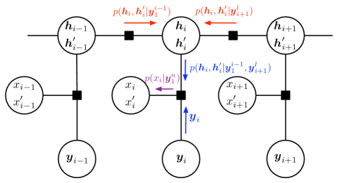
Figure 1: A factor graph describing the communication system model without channel coding. The arrows refer to messages which are discussed in Section III-B

Generally, a factor graph is a bipartite graph, which consists of two types of nodes: the variable nodes, each denoted by a circle in the graph, which represents one or a few random variables jointly; and the factor nodes, each denoted by a square which represents a constraint on the variable nodes connected to it [3, 19]. The factor node between the node $(\boldsymbol{h}_{i},\boldsymbol{h}^{\prime}_{i})$ and the node $(\boldsymbol{h}_{i-1},\boldsymbol{h}^{\prime}_{i-1})$ represents the conditional distribution $p(\boldsymbol{h}_{i},\boldsymbol{h}^{\prime}_{i}|\boldsymbol{h}_{i-1},\boldsymbol{h}^{\prime}_{i-1})$, which is the probability constraint specified by (2). Similarly, the factor node connecting nodes $\boldsymbol{y}_{i}$, $(\boldsymbol{h}_{i},\boldsymbol{h}^{\prime}_{i})$ and $(x_{i},x_{i}^{\prime})$ represents the conditional distribution $p(\boldsymbol{y}_{i}|\boldsymbol{h}_{i},\boldsymbol{h}^{\prime}_{i},x_{i},x_{i}^{\prime})$, which is the relation given by (1). The prior probability distribution of the data symbols is assigned as follows. All BPSK symbols $x_{i}$ and $x^{\prime}_{i}$ are uniformly distributed on $\{-1,1\}$ except for the subset of pilot symbols in $x^{l}_{1}$, which are set to 1. The Markovian property of the graph is that conditioned on any cut node(s), the separated subsets of variables are mutually independent. As we shall see, the Markovian property plays an important role in the development of the message-passing algorithm.

Since the graphical model in Fig. 1 fully describes the probability laws of the random variables given in (1) and (2), the detection problem is equivalent to statistical inference on the graph. Simply put, we seek to answer the following question: Once the realization of a subset of the variables (received signal and pilots) on the graph is revealed, what can be inferred about the symbols from the desired user?

Note that the same factor graph would arise if we were to jointly detect both $x_{i}$ and $x^{\prime}_{i}$, which solves a problem of multiuser detection. In this work, however, the receiver is only interested in detecting $x_{i}$, so that $x_{i}^{\prime}$ is being averaged out when passing messages between nodes $(\boldsymbol{h}_{i},\boldsymbol{h}_{i}^{\prime})$ and $(\boldsymbol{h}_{i+1},\boldsymbol{h}_{i+1}^{\prime})$.

III-B Exact Inference via Message Passing

In the problem described in Section II, the goal of inference is to obtain or approximate the marginal posterior probability $p(x_{i}|\boldsymbol{y}_{1}^{l})$, which is in fact a sufficient statistic of $\boldsymbol{y}_{1}^{l}$ for $x_{i}$. Problems of such nature have been widely studied (see e.g., [22, Chapter 4] and [3]). In particular, BP is an efficient algorithm for computing the posteriors by passing messages among neighboring nodes on the graph. In principle, the result of message passing with sufficient number of steps gives the exact a posteriori probability of each unknown random variable if the factor graph is a tree (i.e., free of cycles). For general graphs with few short cycles, iterative message-passing algorithms often compute good approximations of the desired probabilities. Unlike in most other work (including [13, 14, 15]), where each random variable is made a variable node, multiple variables are clustered into a single node so that the factor graph in Fig. 1 is free of cycles (see also [3] for the usage of the clustering techniques). Numerical experiments (omitted here) show that making each variable a separate node leads to poor performance due to a large number of short cycles (e.g., there will be a cycle through $\boldsymbol{h}_{i},\boldsymbol{h}_{i},\boldsymbol{h}_{i+1},\boldsymbol{h}_{i+1}^{\prime}$).

Let $\boldsymbol{G}_{i}=[\boldsymbol{h}_{i},\boldsymbol{h}^{\prime}_{i}]$ and $\boldsymbol{U}_{i}=[\boldsymbol{w}_{i},\boldsymbol{w}^{\prime}_{i}]$. The model (1) and (2) can be rewritten as:

$$\boldsymbol{y}_{i} =\boldsymbol{G}_{i}\begin{bmatrix}x_{i}\\ x^{\prime}_{i}\end{bmatrix}+\boldsymbol{n}_{i}$$ (3)

$$\boldsymbol{G}_{i} =\alpha\boldsymbol{G}_{i-1}+\sqrt{1-\alpha^{2}}\,\boldsymbol{U}_{i}.$$ (4)

The probability distributions immediately available are $p(\boldsymbol{y}_{i}|\boldsymbol{G}_{i},x_{i},x^{\prime}_{i})$, $p(\boldsymbol{G}_{i}|\boldsymbol{G}_{i-1})$ and the marginals $p(x_{i})$, $p(x^{\prime}_{i})$, as well as $p(\boldsymbol{G}_{i})$ which are Gaussian. Note that $p(\boldsymbol{y}_{i}|\boldsymbol{G}_{i},x_{i},x^{\prime}_{i})$ is the conditional Gaussian density corresponding to the channel model (1) and $p(x_{i},x^{\prime}_{i})=p(x_{i})p(x^{\prime}_{i})$ since the desired symbol and the interference symbol are independent. Also, $P(x_{i}=1)=1$ and $P(x_{i}=-1)=0$ if $x_{i}$ is a pilot for the desired user, otherwise $P(x_{i}=\pm 1)=1/2$. Moreover, $P(x^{\prime}_{i}=\pm 1)\equiv 1/2$ for all $i$, since we do not know the pilot pattern of the interfering user.

The goal is to compute for each $i=1,\dots,l$:

$$p(x_{i}|\boldsymbol{y}_{1}^{l}) =\sum_{x^{\prime}_{i}=\pm 1}\int p(x_{i},x^{\prime}_{i},\boldsymbol{G}_{i}|\boldsymbol{y}_{1}^{l})\,\mathrm{d}\boldsymbol{G}_{i}$$

$$\propto\sum_{x^{\prime}_{i}=\pm 1}\int p(x_{i},x^{\prime}_{i},\boldsymbol{y}_{1}^{i-1},\boldsymbol{y}_{i},\boldsymbol{y}_{i+1}^{l},\boldsymbol{G}_{i})\,\mathrm{d}\boldsymbol{G}_{i}$$

where the “proportion” notation $\propto$ indicates that the two sides differ by a factor which depends only on the observation $\boldsymbol{y}^{l}_{1}$ (which has no influence on the likelihood ratio $P(x_{i}=1|\boldsymbol{y}_{1}^{l})/P(x_{i}=-1|\boldsymbol{y}_{1}^{l})$ and hence on the decision). For notational simplicity we have also omitted the limits of the integrals, which are over the entire axes of $2N_{R}$ complex dimensions. By the Markovian property, $(x_{i},x^{\prime}_{i},\boldsymbol{y}_{i})$, $\boldsymbol{y}_{1}^{i-1}$ and $\boldsymbol{y}_{i+1}^{l}$ are mutually independent given $\boldsymbol{G}_{i}$. Therefore,

$$p(x_{i}|\boldsymbol{y}_{1}^{l}) \propto\sum_{x^{\prime}_{i}=\pm 1}\int p(\boldsymbol{y}_{i},x_{i},x^{\prime}_{i}|\boldsymbol{G}_{i})p(\boldsymbol{y}_{1}^{i-1}|\boldsymbol{G}_{i})$$

$$\hskip 100.00015pt\times p(\boldsymbol{y}_{i+1}^{l}|\boldsymbol{G}_{i})p(\boldsymbol{G}_{i})\,\mathrm{d}\boldsymbol{G}_{i}$$

$$\propto\!\sum_{x^{\prime}_{i}=\pm 1}\!p(x_{i})p(x^{\prime}_{i})\!\!\!\int\!\!p(\boldsymbol{y}_{i}|\boldsymbol{G}_{i},x_{i},x^{\prime}_{i})p(\boldsymbol{G}_{i}|\boldsymbol{y}_{1}^{i-1})$$

$$\hskip 80.00012pt\times p(\boldsymbol{G}_{i}|\boldsymbol{y}_{i+1}^{l})\big{/}p(\boldsymbol{G}_{i})\mathrm{d}\boldsymbol{G}_{i}$$ (5)

where the independence of $(x_{i},x^{\prime}_{i})$ and $\boldsymbol{G}_{i}$ is used to obtain (5). In order to compute (5), it suffices to compute $p(\boldsymbol{G}_{i}|\boldsymbol{y}_{1}^{i-1})$ and $p(\boldsymbol{G}_{i}|\boldsymbol{y}_{i+1}^{l})$.

We briefly derive the posterior probability $p(\boldsymbol{G}_{i}|\boldsymbol{y}^{i-1}_{1})$ as a recursion in below, whereas computation of $p(\boldsymbol{G}_{i}|\boldsymbol{y}_{i+1}^{l})$ is similar by symmetry. Consider the posterior of the coefficients $\boldsymbol{G}_{i}$ given the received signal up to time $i-1$. The influence of $\boldsymbol{y}_{1}^{i-1}$ on $\boldsymbol{G}_{i}$ is through $\boldsymbol{G}_{i-1}$ because $\boldsymbol{G}_{i}$ and $\boldsymbol{y}_{1}^{i-1}$ are independent given $\boldsymbol{G}_{i-1}$. Thus,

$$p(\boldsymbol{G}_{i}|\boldsymbol{y}^{i-1}_{1})=\int p(\boldsymbol{G}_{i}|\boldsymbol{G}_{i-1})p(\boldsymbol{G}_{i-1}|\boldsymbol{y}^{i-1}_{1})\mathrm{d}\boldsymbol{G}_{i-1}\,.$$

By the Markovian property, $\boldsymbol{y}^{i-2}_{1}$ and $\boldsymbol{y}_{i-1}$ are independent given $\boldsymbol{G}_{i-1}$, so that

$$p(\boldsymbol{G}_{i}|\boldsymbol{y}^{i-1}_{1})\!\!\propto\!\!\!\int\!\!p(\boldsymbol{G}_{i}|\boldsymbol{G}_{i-1})p(\boldsymbol{y}_{i-1}|\boldsymbol{G}_{i-1})p(\boldsymbol{G}_{i-1}|\boldsymbol{y}^{i-2}_{1})\mathrm{d}\boldsymbol{G}_{i-1}.$$ (6)

Since $\boldsymbol{G}_{i-1}$ and $x_{i-1},x^{\prime}_{i-1}$ are independent,

$$p (\boldsymbol{y}_{i-1}|\boldsymbol{G}_{i-1})$$

$$=\sum_{x_{i-1},x^{\prime}_{i-1}=\pm 1}p(\boldsymbol{y}_{i-1}|x_{i-1},x^{\prime}_{i-1},\boldsymbol{G}_{i-1})p(x_{i-1})p(x^{\prime}_{i-1})\,.$$ (7)

Therefore, by (6) and (7), we have a recursion for computing $p(\boldsymbol{G}_{i}|\boldsymbol{y}^{i-1}_{1})$ for each $i=1,\dots,l$,

$$p(\boldsymbol{G}_{i}|\boldsymbol{y}^{i-1}_{1})\propto\sum_{x_{i-1},x^{\prime}_{i-1}=\pm 1}\int p(\boldsymbol{G}_{i}|\boldsymbol{G}_{i-1})p(\boldsymbol{G}_{i-1}|\boldsymbol{y}^{i-2}_{1})\\ \times p(\boldsymbol{y}_{i-1}|\boldsymbol{G}_{i-1},x_{i-1},x^{\prime}_{i-1})p(x_{i-1})p(x^{\prime}_{i-1})\,\mathrm{d}\boldsymbol{G}_{i-1}$$ (8)

which is the key to the message-passing algorithm. Similarly, we can also derive the inference on $\boldsymbol{G}_{i}$, which serves as an estimate of channel coefficients at time $i$:

$$p(\boldsymbol{G}_{i}|\boldsymbol{y}_{1}^{l})\propto\sum_{x_{i},x^{\prime}_{i}=\pm 1}p(x_{i})p(x^{\prime}_{i})p(\boldsymbol{y}_{i}|\boldsymbol{G}_{i},x_{i},x^{\prime}_{i})\\ \times p(\boldsymbol{G}_{i}|\boldsymbol{y}_{1}^{i-1})p(\boldsymbol{G}_{i}|\boldsymbol{y}_{i+1}^{l})/p(\boldsymbol{G}_{i}).$$ (9)

In other words, the BP algorithm requires backward and forward message-passing only once in each direction, which is similar to the BCJR algorithm [23]. The key difference between our algorithm and the BCJR is that the Markov chain here has a continuous state space.

The joint channel estimation and interference mitigation algorithm is summarized in Algorithm 1. Basically, the message from a factor node to a variable node is a summary of the extrinsic information (EI) about the random variable(s) represented by the variable node based on all observations connected directly or indirectly to the factor node [3]. For example, the message received by node ($\boldsymbol{h}_{i},\boldsymbol{h}^{\prime}_{i}$) from the factor node on its left summarizes all information about ($\boldsymbol{h}_{i},\boldsymbol{h}^{\prime}_{i}$) based on the observations $\boldsymbol{y}_{1},\ldots,\boldsymbol{y}_{i-1}$, which is proportional to $p(\boldsymbol{h}_{i},\boldsymbol{h}^{\prime}_{i}|\boldsymbol{y}^{i-1}_{1})$. The message from a variable node to a factor node is a summary of the EI about the variable node based on the observations connected to it. For example, the message passed by node ($\boldsymbol{h}_{i},\boldsymbol{h}^{\prime}_{i}$) to the factor node on its left is the EI about ($\boldsymbol{h}_{i},\boldsymbol{h}^{\prime}_{i}$) based on the observations $\boldsymbol{y}_{1},\ldots,\boldsymbol{y}_{i}$, i.e., $p(\boldsymbol{h}_{i},\boldsymbol{h}^{\prime}_{i}|\boldsymbol{y}^{i}_{1})$.

Algorithm 1 Pseudo code for the message-passing algorithm

  Initialization: $P(x^{\prime}_{i}=1)=P(x^{\prime}_{i}=-1)=1/2$ for all $i$. The same probabilities are also assigned to $p(x_{i})$ for all $i$ except for the pilots, for which $P(x_{i}=1)=1$. For all $i$, $p(\boldsymbol{G}_{i})$ is zero mean Gaussian with variance $\boldsymbol{Q}$.

  for $i=1$ to $l$ do

     Compute $p(\boldsymbol{G}_{i}|\boldsymbol{y}^{i-1}_{1})$ from (8)

     Compute $p(\boldsymbol{G}_{i}|\boldsymbol{y}_{i+1}^{l})$ similarly to (8)

  end for

  for $i=1$ to $l$ do

     Compute $p(x_{i}|\boldsymbol{y}_{1}^{l})$ from (5)

  end for

Given the factor graph, it becomes straightforward to write out the message passing algorithm, which is equivalent to the sum-product algorithm [3]. Because of the simple Markovian structure of the factor graph, we derive the algorithm using basic probability arguments in this section. The preceding treatment is self-contained, and the technique also applies to other similar problems.

III-C Practical Issues

Algorithm 1 cannot be implemented directly using a digital computer because the messages are continuous probability density functions (PDFs). Here we choose to parametrize the PDFs, as opposed to quantizing the multi-dimensional PDFs directly, which requires a large number of quantization bins and thus high computational complexity. Also, parametrization can characterize the PDFs exactly without introducing extra quantization error. Thus it can achieve better performance with less complexity. (Of course, for hardware implementation the PDF parameters must be quantized.)

For notational convenience, we use $\boldsymbol{g}$ to denote the column vector formed by stacking the columns of the matrix $\boldsymbol{G}$, i.e., if $\boldsymbol{G}_{i}=[\boldsymbol{h}_{i},\boldsymbol{h}^{\prime}_{i}]$ is $N_{R}\times 2$ as defined previously then $\boldsymbol{g}_{i}=\left[\boldsymbol{h}_{i}^{\mathrm{T}},\boldsymbol{h}^{\prime\mathrm{T}}_{i}\right]^{\mathrm{T}}$ is $2N_{R}\times 1$. We define

$$\boldsymbol{Z}_{i}=\left[x_{i},x^{\prime}_{i}\right]\otimes\boldsymbol{I}_{2}=\begin{bmatrix}x_{i}&0&x^{\prime}_{i}&0\\ 0&x_{i}&0&x^{\prime}_{i}\end{bmatrix}$$

where $\otimes$ denotes the Kronecker product and $\boldsymbol{I}_{r}$ denotes the $r\times r$ identity matrix. Then (3) and (4) are equivalent to

$$\boldsymbol{y}_{i} =\boldsymbol{Z}_{i}\boldsymbol{g}_{i}+\boldsymbol{n}_{i}$$ (10)

$$\boldsymbol{g}_{i} =\alpha\boldsymbol{g}_{i-1}+\sqrt{1-\alpha^{2}}\,\boldsymbol{u}_{i}$$ (11)

where $\boldsymbol{u}_{i}$ is a column vector consisting of $2N_{R}$ independent CSCG variables with variance $\sigma_{h}^{2}$ or $\sigma_{h^{\prime}}^{2}$. Let the $r-$dimensional complex Gaussian density be denoted by

$$\mathcal{CN}(\boldsymbol{x},\boldsymbol{m},\boldsymbol{K})\equiv\frac{1}{\pi^{r}\det(\boldsymbol{K})}\exp\left[-(\boldsymbol{x}-\boldsymbol{m})^{\mathrm{H}}\boldsymbol{K}^{-1}(\boldsymbol{x}-\boldsymbol{m})\right]$$

where $\boldsymbol{x}_{r\times 1}$ is a column vector of complex dimension $r$, and $\boldsymbol{m}_{r\times 1}$ and $\boldsymbol{K}_{r\times r}$ denote the mean and covariance matrix, respectively. Let $\boldsymbol{Q}=\text{diag}(\sigma^{2}_{h},\sigma^{2}_{h},\sigma^{2}_{h^{\prime}},\sigma^{2}_{h^{\prime}})$. We can then write $p(\boldsymbol{g}_{i}|\boldsymbol{g}_{i-1})=\mathcal{CN}(\boldsymbol{g}_{i},\alpha\boldsymbol{g}_{i-1},\sqrt{1-\alpha^{2}}\,\boldsymbol{Q})$, $p(\boldsymbol{g}_{i})=\mathcal{CN}(\boldsymbol{g}_{i},0,\boldsymbol{Q})$ and $p(\boldsymbol{y}_{i}|\boldsymbol{g}_{i},x_{i},x^{\prime}_{i})=\mathcal{CN}(\boldsymbol{y}_{i},\boldsymbol{Z}_{i}\boldsymbol{g}_{i},\sigma^{2}_{n}\boldsymbol{I})$.

The density functions, $p(\boldsymbol{g}_{i}|\boldsymbol{y}_{i+1}^{l})$ and $p(\boldsymbol{g}_{i}|\boldsymbol{y}_{1}^{i-1})$ are Gaussian mixtures. Note that the random variables in Fig. 1 are either Gaussian or discrete. The forward recursion (8) for $p(\boldsymbol{g}_{i}|\boldsymbol{y}_{1}^{i-1})$ starts with a Gaussian density function. As the message is passed from node to node, it becomes a mixture of more and more Gaussian densities. Each Gaussian mixture is completely characterized by the amplitudes, means and variances of its components. Therefore, we can compute and pass these parameters instead of PDFs.

Without loss of generality, we assume that $p(\boldsymbol{g}_{i-1}|\boldsymbol{y}^{i-2}_{1})=\sum_{j}\rho_{j}\,\mathcal{CN}(\boldsymbol{g}_{i-1},\boldsymbol{m}^{j}_{i-1},\boldsymbol{K}^{j}_{i-1})$, where non-negative numbers $\{\rho_{j}\}$ satisfy $\sum_{j}\rho_{j}=1$. Substituting into (8), after some manipulations, we have

$$p(\boldsymbol{g}_{i}|\boldsymbol{y}^{i-1}_{1})\propto\sum_{j,x_{i-1},x^{\prime}_{i-1}}\rho_{j}\,p(x_{i-1})p(x^{\prime}_{i-1})L(j,i)C(j,i)$$ (12)

where

$$L(j,i)=\mathcal{CN}(\boldsymbol{Z}_{i-1}\boldsymbol{m}^{j}_{i-1},\boldsymbol{y}_{i-1},\sigma^{2}_{n}\boldsymbol{I}+\boldsymbol{Z}_{i-1}\boldsymbol{K}^{j}_{i-1}\boldsymbol{Z}_{i-1})$$ (13)

and

$$C(j,i)=\mathcal{CN}\left(\boldsymbol{g}_{i},\boldsymbol{m}^{j,i}_{i},\boldsymbol{K}^{j,i}_{i}\right)$$ (14)

where

$$\boldsymbol{m}^{j,i}_{i} =\alpha\boldsymbol{m}^{j}_{i-1}+\alpha\boldsymbol{K}^{j}_{i-1}\boldsymbol{Z}_{i-1}^{\mathrm{H}}(\sigma^{2}_{n}\boldsymbol{I}+\boldsymbol{Z}_{i-1}\boldsymbol{K}^{j}_{i-1}\boldsymbol{Z}_{i-1})^{-1}$$

$$\hskip 100.00015pt\times(\boldsymbol{y}_{i}-\boldsymbol{Z}_{i-1}\boldsymbol{m}^{j}_{i-1})$$ (15a)

$$\boldsymbol{K}^{j,i}_{i} =\alpha^{2}\boldsymbol{K}^{j}_{i-1}+\sqrt{1-\alpha^{2}}\,\boldsymbol{Q}-(\alpha\boldsymbol{K}^{j}_{i-1}\boldsymbol{Z}_{i-1}^{\mathrm{H}})$$

$$\hskip 10.00002pt\times(\sigma^{2}_{n}\boldsymbol{I}+\boldsymbol{Z}_{i-1}\boldsymbol{K}^{j}_{i-1}\boldsymbol{Z}_{i-1}^{\mathrm{H}})^{-1}(\alpha\boldsymbol{Z}_{i-1}\boldsymbol{K}^{j}_{i-1}).$$ (15b)

Basically, (12), (13) and (14) give an explicit recursive computation for the amplitude, mean and variance of each Gaussian component in message $p(\boldsymbol{g}_{i}|\boldsymbol{y}^{i-1}_{1})$. Similar computations can be applied to $p(\boldsymbol{g}_{i}|\boldsymbol{y}_{i+1}^{l})$.

Examining (15a) and (15b) more closely, ignoring the superscripts, they are the one-step prediction equation and Riccati equations, respectively, for the linear system defined by (3) and (4) with known $\boldsymbol{Z}_{i-1}$ [24, Ch.3], [3, Sec. IV.C]. Therefore, passing messages from one end to the other can be viewed as a series of Kalman filters with different weights: In each step, each filter performs the traditional Kalman filter for each hypothesis of $\boldsymbol{Z}_{i-1}$ and the filtered result is weighted by the product of the previous weight, the posterior probability of the hypothesis, and $L(j,i)$.

The number of Gaussian components increases exponentially in the recursive formula (12), which becomes computationally infeasible. In this work, we fix the total number of components and simply pick the components with the largest amplitudes (which correspond to the most likely hypotheses). In general, this problem is equivalent to the problem of survivor-reduction. Two techniques that have been proposed are decision feedback [26] and thresholding [27]. The former limits the maximum number of survivors by assuming the past decisions are correct, while the latter keeps the survivors only when their a posteriori probabilities exceed a certain threshold value. According to the preceding analysis, the method we propose falls into the decision feedback category. Obviously, the more components we keep, the better performance we have; however, the higher the complexity at the receiver. We investigate this issue numerically in Section VI. A different approach to limiting the number of Gaussian components is presented in [28, 29, 30, 14, 31]. There the basic idea is to merge components “close” to each other instead of discarding the weakest ones as we do here. However, that requires computing distances between pairs of components, which can lead to significantly higher complexity [31, 29]. The relative performance of these different methods is left for future study.

III-D Integration with Channel Coding

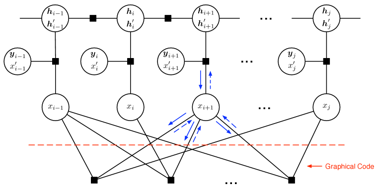
Figure 2: A factor graph for joint detection, estimation and decoding. The solid arrows show EI passed from the detector to the decoder, and the dashed arrows show EI passed from the decoder to the detector.

Channel codes based on factor graphs can be easily incorporated in the message-passing framework developed thus far. In Fig. 2, a sparse graphical code is in conjunction with the factor graph for the model (1) and (2). The larger factor graph is no longer acyclic. Therefore, the message-passing algorithm is sub-optimal for this graph even if one could keep all detection hypotheses (i.e., the number of mixture components is unrestrained). However, design of channel coding can guarantee the degrees of such cycles are typically quite large. Hence message-passing performs very well [5]. Based on the factor graph, one can develop many message-passing schedules. To exploit the slow variation of the fading channel, the non-Gaussian property of the interfering signal and the structure of graphical codes, a simple idea is to allow the detector and decoder to exchange their extrinsic information. For example, suppose that at a certain message-passing stage, the node $x_{i+1}$ computes its APP from the detector. Then the node $x_{i+1}$ can distribute the EI to the sub-graph of the graphical code, which is described by the solid arrows in Fig. 2. After $x_{i+1}$ collects the “beliefs” from all its edges, it passes the EI (which is obtained by multiplying together all “beliefs” but the one coming from the detector) back to the detector. This process is described by the dashed arrows in Fig. 2. In other words, both the detector and the decoder compute their posterior probabilities from received EI.

In this paper, we use LDPC codes with the following simple strategy: We run the detection part as before and then feed the EI to the LDPC decoder through variable nodes $x_{i}$. After running the LDPC decoder several rounds, we feed back the EI to the detection sub-graph. We investigate the impact of the message-passing schedule on performance numerically in Section VI.

IV Error Floor Due to Channel Uncertainty

Channel variations impose a fundamental limit on the error performance regardless of the signal-to-noise ratio (SNR). Consider a genie-aided receiver: when detecting symbol $x_{i}$, a genie reveals all channel coefficients but $(\boldsymbol{h}_{i},\boldsymbol{h}^{\prime}_{i})$ to the receiver, which can only reduce the minimum error probability. Even in the absence of noise, the receiver cannot estimate $(\boldsymbol{h}_{i},\boldsymbol{h}^{\prime}_{i})$ precisely (not even the sign) due to the Markovian property in (2). Therefore, the error probability does not vanish as the noise power goes to zero.

Evidently, the genie-aided receiver also gives a lower bound on the error probability for the exact message passing algorithm. In the following, we derive an approximation to this lower bound. Numerical results in Section V indicate that the difference between the approximate lower bound and the actual genie-aided performance is small.

Consider the error probability of jointly detecting $[x_{i},x^{\prime}_{i}]$ with the help of the genie. Conditioned on all other channel coefficients, $\boldsymbol{h}_{i}$ and $\boldsymbol{h}^{\prime}_{i}$ are Gaussian. Let $\boldsymbol{h}_{i}=\hat{\boldsymbol{h}}_{i}+\tilde{\boldsymbol{h}}_{i}$ and $\boldsymbol{h}^{\prime}_{i}=\hat{\boldsymbol{h}}^{\prime}_{i}+\tilde{\boldsymbol{h}}^{\prime}_{i}$ where $\hat{\boldsymbol{h}}_{i}$ and $\hat{\boldsymbol{h}}^{\prime}_{i}$ are the estimates of $\boldsymbol{h}_{i}$ and $\boldsymbol{h}^{\prime}_{i}$, respectively, and $\tilde{\boldsymbol{h}}_{i}$ and $\tilde{\boldsymbol{h}}_{i}$ are the respective estimation errors. By treating $\tilde{\boldsymbol{h}}_{i}x_{i}$ and $\tilde{\boldsymbol{h}}^{\prime}_{i}x^{\prime}_{i}$ as additional noise, the channel model can be rewritten as

$$\boldsymbol{y}_{i}=\hat{\boldsymbol{h}}_{i}x_{i}+\hat{\boldsymbol{h}}^{\prime}_{i}x^{\prime}_{i}+\tilde{\boldsymbol{n}}_{i}$$

where the residual noise $\tilde{\boldsymbol{n}}_{i}=\tilde{\boldsymbol{h}}_{i}x_{i}+\tilde{\boldsymbol{h}}^{\prime}_{i}x^{\prime}_{i}+\boldsymbol{n}_{i}$. It can be shown that $\tilde{\boldsymbol{n}}_{i}$ is a CSCG random vector independent of $(x_{i},x^{\prime}_{i})$ and with covariance matrix $\sigma_{\tilde{n}}^{2}\boldsymbol{I}=\left(\frac{1-\alpha^{2}}{1+\alpha^{2}}(\sigma_{h}^{2}+\sigma_{h^{\prime}}^{2})+\sigma_{n}^{2}\right)\boldsymbol{I}$.

Let $\hat{x}_{i}$ and $\hat{x}^{\prime}_{i}$ be the estimates of $x_{i}$ and $x^{\prime}_{i}$, respectively. For simplicity, we assume dual receive antennas ($N_{R}=2$). Following a standard analysis [1, App. A], we have

$$P(\text{error}) =P(\hat{x}_{i}\neq x_{i},\hat{x}^{\prime}_{i}=x^{\prime}_{i})+P(\hat{x}_{i}\neq x_{i},\hat{x}^{\prime}_{i}\neq x^{\prime}_{i})$$

$$=\left(\frac{1-\mu_{1}}{2}\right)^{2}\!\!(2+\mu_{1})+\left(\frac{1-\mu_{2}}{2}\right)^{2}(2+\mu_{2})$$ (16)

where

$$\mu_{1} =\sqrt{\frac{\alpha^{2}\sigma_{h}^{2}}{\alpha^{2}\sigma_{h}^{2}+(1+\alpha^{2})\sigma_{\tilde{n}}^{2}}}$$

$$\mu_{2} =\sqrt{\frac{\alpha^{2}(\sigma_{h}^{2}+\sigma_{h^{\prime}}^{2})}{\alpha^{2}(\sigma_{h}^{2}+\sigma_{h^{\prime}}^{2})+(1+\alpha^{2})\sigma_{\tilde{n}}^{2}}}\,.$$

Note that as long as $\alpha\neq 1$, the residual noise $\tilde{n}$ does not vanish, which results in an error floor. Therefore, such error floor is inherent to the channel model, and despite its simplicity, the channel cannot be tracked exactly based on pilots.

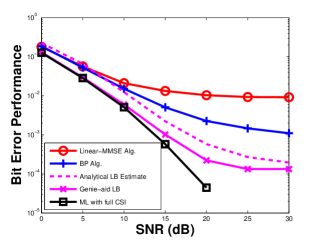
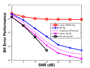
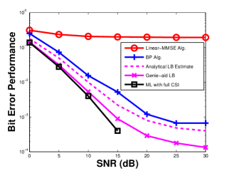
Figure 3: The BER performance of the message-passing algorithm. The density of pilots is 25%. (a) The power of the interference is 10 dB weaker than that of the desired user. (b) The power of the interference is 3 dB weaker than that of the desired user. (c) The power of the interference is identical to that of the desired user.

V Extensions and Complexity

V-A Extensions

The message-passing approach applies to general multiple-input multiple-output systems. For example, if $N_{T}$ transmit antennas are used by the desired user, $N^{\prime}_{T}$ transmit antennas are used by the interferer, and $N_{R}$ antennas are used by the receiver, then the system can be described as

$$\boldsymbol{y}_{i} =\boldsymbol{H}_{i}\boldsymbol{x}_{i}+\boldsymbol{H}^{\prime}_{i}\boldsymbol{x}^{\prime}_{i}+\boldsymbol{n}_{i}$$ (17a)

$$\boldsymbol{H}_{i} =\boldsymbol{F}\boldsymbol{H}_{i-1}+\boldsymbol{W}_{i}$$ (17b)

$$\boldsymbol{H}^{\prime}_{i} =\boldsymbol{F}^{\prime}\boldsymbol{H}^{\prime}_{i-1}+\boldsymbol{W}^{\prime}_{i}$$ (17c)

where $\boldsymbol{y}_{i}(N_{R}\times 1)$, $\boldsymbol{x}_{i}(N_{T}\times 1)$, $\boldsymbol{x}^{\prime}_{i}(N^{\prime}_{T}\times 1)$ are the received signal, desired user’s signal and interfering signal, respectively, at time $i$, the noise $\boldsymbol{n}_{i}(N_{R}\times 1)$ consists of CSCG entries, and $\boldsymbol{H}_{i}(N_{R}\times N_{T})$ and $\boldsymbol{H}_{i}(N_{R}\times N^{\prime}_{T})$ are independent channel matrices. Equations (17b) and (17c) represent the evolution of the channels, where $\boldsymbol{F}$ and $\boldsymbol{F}^{\prime}$ are in general square matrices, and $\boldsymbol{W}_{i}$ and $\boldsymbol{W}^{\prime}_{i}$ are independent CSCG noises.

Let $\boldsymbol{h}_{j,i}$ represent the $j$-th column of $\boldsymbol{H}_{i}$, and define

$$\boldsymbol{g}_{i} =\left[\boldsymbol{h}_{1,i}^{\mathrm{T}},\boldsymbol{h}^{\mathrm{T}}_{2,i},\dots,\boldsymbol{h}^{\mathrm{T}}_{N_{T},i},\boldsymbol{h}^{\prime\mathrm{T}}_{1,i},\boldsymbol{h}^{\prime\mathrm{T}}_{2,i},\dots,\boldsymbol{h}^{\prime\mathrm{T}}_{N^{\prime}_{T},i}\right]^{\mathrm{T}}$$

$$\boldsymbol{u}_{i} =\left[\boldsymbol{w}^{\mathrm{T}}_{1,i},\boldsymbol{w}^{\mathrm{T}}_{2,i},\dots,\boldsymbol{w}^{\mathrm{T}}_{N_{T},i},\boldsymbol{w}^{\prime\mathrm{T}}_{1,i},\boldsymbol{w}^{\prime\mathrm{T}}_{2,i},\dots,\boldsymbol{w}^{\prime\mathrm{T}}_{N^{\prime}_{T},i}\right]^{\mathrm{T}}$$

$$\boldsymbol{Z}_{i} =\left[\boldsymbol{x}^{\mathrm{T}}_{i},\boldsymbol{x}^{\prime\mathrm{T}}_{i}\right]^{\mathrm{T}}\otimes\boldsymbol{I}_{N_{R}}$$

$$\boldsymbol{A} =\mathbb{E}\left[\boldsymbol{g}_{i}\boldsymbol{g}^{\mathrm{H}}_{i-1}\right]\left(\mathbb{E}[\boldsymbol{g}_{i-1}\boldsymbol{g}^{\mathrm{H}}_{i-1}]\right)^{-1}$$

$$\boldsymbol{B} =\mathbb{E}[\boldsymbol{g}_{i}\boldsymbol{u}_{i}^{\mathrm{H}}]\,.$$

Note that (10) and (11) are still valid, where $\alpha$ and $\sqrt{1-\alpha^{2}}\,\boldsymbol{Q}$ are replaced by $\boldsymbol{A}$ and $\boldsymbol{B}$, respectively. Therefore, with this replacement, the BP algorithm for this general model remains the same.

We can also replace the Gauss-Markov model with higher order Markov models. By expanding the state space (denoted by $\boldsymbol{G}_{i}$), we can still construct the corresponding factor graph by replacing variable nodes $(\boldsymbol{H}_{i},\boldsymbol{H}^{\prime}_{i})$ with $\boldsymbol{G}_{i}$, and a similar algorithm can be derived as before. Also, extensions to systems with more than one interference can be similarly derived.

Furthermore, the proposed scheme can in principle be generalized to any signal constellation and any space-time codes, including QPSK, 8-PSK, 16-QAM and Alamouti codes. However, as the constellation size, the space-time codebook size or the number of interferers increases, the complexity of the algorithm increases rapidly, while the advantage over linear channel estimation vanishes because the interference becomes more Gaussian due to central limit theorem. Thus the algorithm proposed in this paper is particularly suitable for BPSK and QPSK modulations, space-time codewords with short block length and a small number of interferers. A detailed tally of the total complexity is given next.

V-B Complexity

With or without coding, the complexity of the message-passing receiver is linear in the frame length, and polynomial in the number of antennas.

Suppose that there are $m$ channel coefficients, so $\boldsymbol{g}$ is a vector of length $m$ (for the Gauss-Markov channel model $m=N_{R}(N_{T}+N^{\prime}_{T})$). The number of receive antennas is $N_{R}$, the maximum number of Gaussian components we allow is $C$, and the sizes of the alphabet of $x_{i}$ and $x^{\prime}_{i}$ are $|\mathcal{A}|$ and $|\mathcal{A^{\prime}}|$, respectively. The complexity of computing $p(\boldsymbol{g}_{i}|\boldsymbol{y}^{i-1}_{1})$ is then $O(C|\mathcal{A}||\mathcal{A^{\prime}}|N^{a}_{R}l)$, where $l$ is the frame length and $N^{a}_{R}$ is due to the matrix inverse in (15b). The exponent $a$ depends on the particular inversion algorithm, and is typically between two and three. Similar complexity is needed to compute $p(\boldsymbol{G}_{i}|\boldsymbol{y}^{l}_{i+1})$. To synthesize the results from the backward and forward message passing via (5), we need $O(C^{2}|\mathcal{A}||\mathcal{A^{\prime}}|m^{a}l)$ computations. Thus, the total complexity for the uncoded system is $O((CN^{a}_{R}+C^{2}m^{a})|\mathcal{A}||\mathcal{A^{\prime}}|l)$. To reduce the complexity, one can reduce $C$, which causes performance loss. One can also try to approximate the matrix inverse (or equivalently, replace the Kalman filter with a suboptimal filter).

For a coded system, the complexity of message-passing LDPC decoder is generally linear in codeword length [4]. With multiple frames coded into one codeword, the decoder complexity is also linear in the frame length. Suppose the number of EI exchanges between detector and decoder is $I_{det}$. Then the overall complexity for the receiver is $O((CN^{a}_{R}+C^{2}m^{a})I_{det}|\mathcal{A}||\mathcal{A^{\prime}}|l)$.

VI Simulation Results

In this section, the model presented in Section II with dual receive antennas ($N_{R}=2$) and BPSK signaling, is used for simulation. The performance of the message-passing algorithm is plotted versus signal-to-noise ratio $SNR=\sigma_{h}^{2}/\sigma_{n}^{2}$, where the covariance matrix of the noise is $\sigma_{n}^{2}\boldsymbol{I}$. We set the channel correlation parameter $\alpha=.99$ and limit the maximum number of Gaussian components to $8$. Within each block, there is one pilot in every $4$ symbols. For the uncoded system, we set the frame length to $l=200$. For the coded system, we use a $(500,250)$ irregular LDPC code and multiplex one LDPC codeword into a single frame, i.e., we do not code across multiple frames.

VI-A Performance of Uncoded System

VI-A1 BER Performance

Results for the message-passing algorithm with the Gaussian mixture messages described in Section III are shown in Figs. 3 to 8. We also show the performance of three other receivers for comparison. The first is denoted by “MMSE”, which estimates the desired channel by taking a linear combination of adjacent received value. This MMSE estimator treats the interference as white Gaussian noise. The second is the genie-aided receiver described in Section IV, denoted by “Genie-aided LB”, which gives a lower bound on the performance of the message-passing algorithm. The third one is denoted by “ML with full CSI”, which performs maximum likelihood detection for each symbol assuming that the realization of the fading processes is revealed to the detector by a genie, which lower bounds the performance of all other receivers. We also plot the approximation of the BER for the optimal genie-aided receiver obtained from (IV) using a dashed line.

Fig. 3 shows uncoded BER vs. SNR, where the power of the interference is $10$ dB weaker, $3$ dB weaker and equal to that of the desired user, respectively. The message-passing algorithm generally gives a significant performance gain over the MMSE channel estimator, especially in the high SNR region. Note that thermal noise dominates when the interference is weak. Therefore, relatively little performance gain over the MMSE algorithm is observed in Fig. 3. In the very low SNR region, the MMSE algorithm slightly outperforms the message-passing algorithm, which is probably due to the limitation on number of Gaussian components.

The trend of the numerical results shows that the message-passing algorithm effectively mitigates or partially cancels the interference at all SNRs of interest, as opposed to suppressing it by linear filtering. We see that there is still a gap between the performance of the message-passing algorithm and that of the genie-aided receiver. The reason is that revealing the channel coefficients enables the receiver to detect the symbol of the interferer with improved accuracy. Another observation is that the analytical estimate is closer to the message-passing algorithm performance with stronger interference.

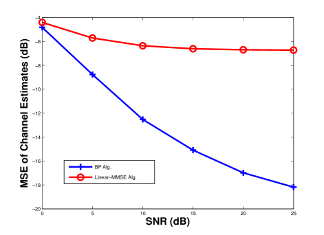
Figure 4: Channel estimation error with an interferer, which is 3 dB weaker than the desired signal. The density of pilots is 25%.

VI-A2 Channel Estimation Performance

The channel estimate from the message-passing algorithm is much more accurate than that from the conventional linear channel estimation. Fig. 4 shows the mean squared error for the channel estimation versus SNR where the interference signal is 3 dB weaker than the desired signal and one pilot is used after every three data symbols. Note that the performance of the linear estimator hardly improves as the SNR increases because the signal-to-interference-and-noise ratio is no better than 3 dB regardless of the SNR. This is the underlying reason for the poor performance of the linear receiver shown in Fig. 3.

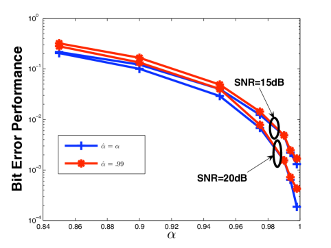
Figure 5: Performance v.s. different values of $\alpha$ with 3 dB weaker interference. For curves marked with “+”, the receiver uses the true value of correlation coefficient i.e., $\hat{\alpha}=\alpha$. For curves marked with “*”, receiver uses $\hat{\alpha}=.99$ regardless of the value of $\alpha$.

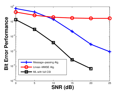
Figure 6: Performance under the Clarke channel with normalized maximum Doppler frequency $0.02$ and 3 dB weaker interference.

VI-B The Impact of Imperfect Knowledge of Channel Statistics

Although the statistical model for the channel is usually determined a priori, the parameters of the model are often based on on-line estimates, which may be inaccurate. The following simulations evaluate the robustness of the receiver when some parameters, or the model itself is not accurate. The simulation conditions here are the same as for the previous uncoded system with 3 dB weaker interference. Fig. 5 plots the BER performance against the correlation coefficient $\alpha$, while the receiver uses $\hat{\alpha}$ instead. It is clear that the mismatch in $\alpha$ causes little degradation. The result of a similar experiment is plotted in Fig. 6, where the receiver assumes the Gauss-Markov model, while the actual channels follow the Clarke model [1, Ch. 2]. We see that the message-passing algorithm still works well. In fact, as long as the channel varies relatively slowly, modeling it as a Gauss-Markov process leads to good performance.

VI-C Coded system and the Impact of Message-passing Schedule

Consider coded transmission using a $(500,250)$ irregular LDPC code and with one LDPC codeword in each frame, i.e., no coding across multiple frames. Since we insert one pilot after every $3$ symbols, the total frame length is $667$ symbols. For the message-passing algorithm, let $I_{det}$ denote the total number of EI exchanges between decoder and detector, and $I_{dec}$ denote the number of iterations of the LDPC decoder during each EI exchange. Different values for pair $(I_{det},I_{dec})$ correspond to different message-passing schedules.

In Fig. 7, we present the performance of two message-passing schedules: (a) $I_{det}=1$ and $I_{dec}=50$ denoted by “Separate Message-passing Alg.”, i.e., the receiver detects the symbol first, then passes the likelihood ratio to the LDPC decoder without any further EI exchanges (separate detection and decoding), and (b) $I_{det}=5$ and $I_{dec}=10$, denoted by “Joint Message-passing Alg.”, i.e., there are five EI exchanges and the LDPC decoder iterates $10$ rounds in between each EI exchange. For the other two receiver algorithms, the total number of iterations of LDPC decoder are both $50$. As shown in Fig. 7, the message-passing algorithm preserves a significant advantage over the traditional linear MMSE algorithm and the joint message-passing algorithm gains even more.

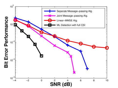
Figure 7: The BER performance for the system with a $(500,250)$ irregular LDPC code. The interference is 3 dB weaker than the desired signal. The density of pilots is 25%. “ML Detection with full CSI” refers to ML detection with full CSI followed by BP-based LDPC decoding, which serves as a performance benchmark.

The performance with different message-passing schedules is shown in Fig. 8. where we fix total number of LDPC iterations $I_{det}\times I_{dec}$. Generally speaking, if $I_{dec}$ or $I_{det}\times I_{dec}$ is fixed, more EI exchanges lead to better performance. We also observe that when $I_{dec}$ is relatively large, say $30$, the performance gain from EI exchanges is small. The reason is that when $I_{dec}$ is large, the output of the LDPC decoder “hardens”, i.e., the decoder essentially decides what each information bit is. When the EI is passed to the detector, all symbols look like pilots from the point of view of the detector. Therefore, there is not much gain in this case.

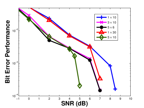
Figure 8: The impact of different message-passing schedules.

VI-D The Impact of Mixture Gaussian Approximation

As previously mentioned, the number of Gaussian components in the messages related to the fading coefficients grows exponentially. For implementation, we often have to truncate or approximate the mixture Gaussian message. In this paper, we keep only a fixed number of components with the maximum amplitudes. The maximum number of components clearly has some impact on the performance. Here we present some numerical experiments to illustrate this effect.

When the pilot density is high, say $50\%$, there is no need to keep many Gaussian components in each message. In fact, keeping two components is essentially enough. However, when the pilot density is lower, say $25\%$, the situation is different. Fig. 9 shows the BER performance when we keep different numbers of Gaussian components in the message-passing algorithm where the pilot density is $25\%$. For this case, we need $8$ components for each message passing step. Indeed, the lower the pilot density, the more Gaussian components we need to achieve the same performance. When the pilot density is low, we must keep a sufficient number of components, corresponding to a sufficient resolution for the message. Roughly speaking, the number of Gaussian components needed is closely related to the number of hypotheses arising from symbols between the symbol of interest and the nearest pilot.

For a single-user system, previous studies indicate that a single Gaussian approximation of the messages is sufficient, e.g., [20]. Fig. 9 shows that this is not the case for the system considered with one dominant interferer. For the simulation with the single Gaussian approximation all Gaussian components are combined into one at each message-passing stage according to the minimum divergence criterion [31]. As expected, the performance with the single Gaussian approximation is relatively poor. Namely, consider the posterior probability, or conditional PDF, of $(\boldsymbol{h}_{i},\boldsymbol{h}_{i}^{\prime})$, which is the message passed along the graph. Due to the lack of pilots for estimating $\boldsymbol{h}^{\prime}_{i}$, there is inherent ambiguity of its polarity so that the posterior of $\boldsymbol{h}^{\prime}_{i}$ is always symmetric around the origin even with an exact message-passing algorithm. Consequently, any approximation with a single Gaussian function can do no better than treating $\boldsymbol{h}^{\prime}_{i}$ as a zero-mean Gaussian random vector. This is equivalent to treating $\boldsymbol{h}^{\prime}_{i}x^{\prime}_{i}$ as Gaussian noise, which leads to poor performance.

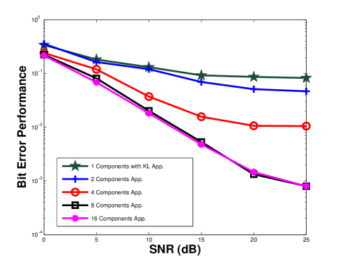
Figure 9: The BER performance with different number of components in the messages. The interference is assumed to be 3 dB weaker than the desired signal. The density of pilots is $25\%$.

VII Conclusion

A novel architecture based on graphical models and belief propagation has been proposed for joint channel estimation, interference mitigation and decoding. Such joint processing is facilitated by efficient iterative message-passing algorithms, where the total complexity is essentially the sum of the complexity of the components, rather than their product as is typical in joint maximum likelihood receivers. In the presence of time-varying Rayleigh fading and a strong co-channel interference, the message-passing algorithm provides a much lower uncoded error floor than linear channel estimation. The results with LDPC codes show at least 5 dB gain for achieving acceptable bit-error rates. Also, this gain is robust with respect to mismatch in channel statistics.

We have considered only two users with multiple receive antennas. Although this is an important case, and the approach can be generalized, there may be implementation (complexity) issues with extending the algorithm. For example, if we have more than one interferer or use larger constellations, the number of hypotheses at each message-passing step increases significantly. To maintain a target performance, we need to increase the number of Gaussian components in each step accordingly. Therefore, the complexity may significantly increase with these extensions. Finally, the algorithm is difficult to analyze. While our results give some basic insights into performance, relative gains are difficult to predict.

Directions for future work include extensions to MIMO channels (where channel modeling within the message-passing framework becomes a challenge) as well as implementation issues including methods for reducing complexity. Extending the message-passing approach to equalization of frequency selective channels with interference is also an interesting direction. For example, the narrowband model (1) considered here could be viewed as an OFDM system with a number of sub-channels. (The receiver algorithm should then be modified to account for correlations across sub-channels.) Alternatively, message-passing approach could be combined with adaptive equalization in the time domain.

References

- [1] D. Tse and P. Viswanath, Fundamentals of Wireless Communications. Cambridge University Press, 2005.
- [2] K. Sil, M. Agarwal, D. Guo, and M. L. Honig, “Performance of Turbo decision-feedback detection and decoding in downlink OFDM,” in Proc. IEEE Wireless Commun. Networking Conf., Mar. 2007.
- [3] F. R. Kschischang, B. J. Frey, and H.-A. Loeliger, “Factor graphs and the sum-product algorithm,” IEEE Trans. Inf. Theory, vol. 47, no. 2, pp. 498–519, Feb. 2001.
- [4] T. J. Richardson and R. L. Urbanke, “The capacity of low-density parity-check codes under message-passing decoding,” IEEE Trans. Inf. Theory, vol. 47, no. 2, pp. 599–618, Feb. 2001.
- [5] T. J. Richardson, M. A. Shokrollahi, and R. L. Urbanke, “Design of capacity-approaching irregular low-density parity-check codes,” IEEE Trans. Inf. Theory, vol. 47, no. 2, pp. 619–637, Feb. 2001.
- [6] A. P. Worthen and W. Stark, “Unified design of iterative receivers using factor graphs,” IEEE Trans. Inf. Theory, vol. 47, no. 2, pp. 843–849, Feb. 2001.
- [7] X. Jin, A. W. Eckford, and T. E. Fuja, “LDPC codes for non-coherent block fading channels with correlation: Analysis and design,” IEEE Trans. Commun., vol. 56, no. 1, pp. 70–80, Jan. 2008.
- [8] C. Komninakis and R. D. Wesel, “Joint iterative channel estimation and decoding in flat correlated Rayleigh fading,” IEEE J. Sel. Areas Commun., vol. 19, no. 9, pp. 1706–1717, Sep. 2001.
- [9] Q. Guo and L. Ping, “LMMSE Turbo equalization based on factor graphs,” IEEE J. Sel. Areas Commun., vol. 26, no. 2, Feb. 2008.
- [10] J. Boutros and G. Caire, “Iterative multiuser joint decoding: Unified framework and asymptotic analysis,” IEEE Trans. Inf. Theory, vol. 48, no. 7, pp. 1772–1793, Jul. 2002.
- [11] D. Guo and T. Tanaka, “Generic multiuser detection and statistical physics,” in Advances in Multiuser Detection, M. L. Honig, Ed. Wiley-IEEE Press, 2009, ch. 5.
- [12] D. Guo and C.-C. Wang, “Multiuser detection of sparsely spread CDMA,” IEEE J. Sel. Areas Commun., vol. 26, no. 4, pp. 421–431, Apr. 2008.
- [13] A. Barbieri, G. Colavolpe, and G. Caire, “Joint iterative detection and decoding in the presence of phase noise and frequency offset,” IEEE Trans. Commun., vol. 55, no. 1, pp. 171–179, Jan. 2007.
- [14] G. Colavope, A. Barbieri, and G. Caire, “Algorithms for iterative decoding in the presence of strong phase noise,” IEEE J. Sel. Areas Commun., vol. 23, no. 9, pp. 1748–1757, Sep. 2005.
- [15] J. Dauwels and H. Loeliger, “Phase estimation by message passing,” in Proc. IEEE Int’l Conf. Commun., Paris, France, Jun. 2004, pp. 523–527.
- [16] I. Abou-Faycal, M. Médard, and U. Madhow, “Binary adaptive coded pilot symbol assisted modulation over Rayleigh fading channels without feedback,” IEEE Trans. Commun., vol. 53, no. 6, pp. 1036–1046, Jun. 2005.
- [17] H. S. Wang and P.-C. Chang, “On verifying the first-order Markovian assumption for a Rayleigh fading channel model,” IEEE Trans. Veh. Technol., vol. 45, no. 2, pp. 353–357, May 1996.
- [18] C. C. Tan and N. C. Beaulieu, “On first-order Markov modeling for the Rayleigh fading channel,” IEEE Trans. Commun., vol. 48, no. 12, pp. 2032–2040, Dec. 2000.
- [19] H.-A. Loeliger, J. Dauwels, J. Hu, S. Korl, L. Ping, and F. R. Kschischang, “The factor graph approach to model-based signal processing,” Proceedings of the IEEE, vol. 95, no. 6, pp. 1295–1322, Jun. 2007.
- [20] H. Niu, M. Shen, J. Ritcey, and H. Liu, “A factor graph approach to iterative channel estimation and LDPC decoding over fading channels,” IEEE Trans. Wireless Commun., vol. 4, no. 4, Jul. 2005.
- [21] G. D. Forney, “Codes on graphs: Normal realizations,” IEEE Trans. Inf. Theory, vol. 47, no. 2, pp. 520–548, Feb 2001.
- [22] D. C. MacKay, Information Theory, Inference and Learning Algorithms. Cambridge University Press, 2003.
- [23] L. R. Bahl, J. Cocke, F. Jelinek, and J. Raviv, “Optimal decoding of linear codes for minimizing symbol error rate,” IEEE Trans. Inf. Theory, vol. 20, no. 2, pp. 284–287, 1974.
- [24] B. D. O. Anderson and J. B. Moore, Optimal Filtering. Dover Publications, Inc., 1979.
- [25] J. Heo and K. M. Chugg, “Adaptive iterative detection for Turbo codes on flat fading channels,” in Proc. Wireless Commun. Networking Conf., vol. 1, Aug. 2000, pp. 134–139.
- [26] S. J. Simmons, “Breadth-first trellis decoding with adaptive effort,” IEEE Trans. Commun., vol. 38, no. 1, pp. 3–12, Jan. 1990.
- [27] Q. Dai and E. Shwedyk, “Detection of bandlimited signals over frequency selective Rayleigh fading channels,” IEEE Trans. Commun., vol. 42, no. 2/3/4, pp. 941–950, Feb./Mar./Apr. 1994.
- [28] J. Dauwels, S. Korl, and H.-A. Loeliger, “Particle methods as message passing,” in Proc. IEEE Int. Symp. Inform. Theory, Jul. 2006, pp. 2052–2056.
- [29] D. W. Scoot and W. F. Szewczyk, “From kernels to mixtures,” Technometrics, vol. 43, no. 3, pp. 323–335, Aug. 2001.
- [30] E. B. Sudderth, A. T. Ihler, W. T. Freeman, and A. S. Willsky, “Nonparametric belief propagation,” in Proc. IEEE Comp. Vision Patt. Recog., vol. 1, Jun. 2003, pp. 605–612.
- [31] B. Kurkoski and J. Dauwels, “Message-passing decoding of lattices using Gaussian mixtures,” in Proc. IEEE Int. Symp. Inform. Theory, 2008, pp. 2489–2493.
- [32] D. Coppersmith and S. Winograd, “Matrix multiplication via arithmetric progressions,” in Proc. 9th Ann. ACM Symp. Theory Comp., 1987, pp. 1–6.
- [33] H. Cohn, R. Kleinberg, B. Szegedy, and C. Umans, “Group-theoretic algorithms for matrix multiplication,” in Proc. IEEE 46th Ann. Found. Comp. Sci., Oct. 2005, pp. 379–388.