Adiabatic dynamics in a spin-1 chain with uniaxial single-spin anisotropy

Abstract

We study the adiabatic quantum dynamics of an anisotropic spin-1 XY chain across a second order quantum phase transition. The system is driven out of equilibrium by performing a quench on the uniaxial single-spin anisotropy, that is supposed to vary linearly in time. We show that, for sufficiently large system sizes, the excess energy after the quench admits a non trivial scaling behavior that is not predictable by standard Kibble-Zurek arguments for isolated critical points or extended critical regions. This emerges from a competing effect of many accessible low-lying excited states, inside the whole continuous line of critical points.

Keywords: Spin chains, ladders and planes (theory); Quantum phase transitions (theory); Density matrix renormalization group calculations

1 Introduction

Recent impressive experimental advances in manipulating cold atoms loaded in optical lattices have opened up the possibility to investigate the actual dynamics of quantum many-body systems with very low dissipation rates and long coherence times [1]; this also allowed a very accurate check of the fundamental laws describing the physics of such systems. Among the others, it has been possible to probe a variety of very interesting and genuinely quantum non-equilibrium phenomena, such as, for example, the collapse and the revival of a Bose-Einstein condensate [2], the manipulation of the atomic number statistics [3], or the coherent non-equilibrium evolution of one-dimensional strongly interacting bosons from a carefully prepared initial state [4]. Furthermore, non-equilibrium in cold atomic gases can also be achieved by changing in time some of the coupling constants of the system, e.g., the depth of the optical lattice or the harmonic trap, on a scale shorter than the relaxation rate. These new experimental capabilities have spurred a renewed interest in the study of quantum quenches.

A lot of attention has been devoted to the study of sudden quenches (see for example [5] and references therein). In this paper we deal with an equally debated problem, i.e., when the changes in the coupling constants driving the quantum system are performed adiabatically. This problem becomes non-trivial if, during the quench, the system crosses a Quantum Phase Transition (QPT). Due to the closure of the gap in the thermodynamic limit, the system will be unable to stay in its equilibrium ground state, no matter how slow is the quench. This problem plays a crucial role in adiabatic quantum computation schemes, where the system Hamiltonian is supposed to be slowly changed on a time scale that is large as compared to the typical inverse zero-temperature gap, so that the system always remains in its instantaneous ground state [6, 7, 8]. The efficiency of an adiabatic quantum computation algorithm relies on the assumption that the minimum gap between the ground state and the first excited state goes gently to zero in the thermodynamic limit. When this is not the case, the non-adiabatic evolution close to the QPT drives the system out of the ground state. The computation is no-longer accurate or, in other words, a number of defects appears in the final state.

The problem of defect formation in the adiabatic dynamics of critical systems was examined much before quantum information: it was first considered by Kibble and Zurek (KZ) in the context of phase transitions in the early universe [9, 10] and more recently extended to the quantum case [11, 12], raising an intense theoretical discussion [13, 14, 15, 16, 17, 18, 19, 20, 21, 22, 23, 24, 25, 26, 27, 28, 29, 30]. According to the KZ mechanism, the evolution of a quantum system is either adiabatic or impulse, depending on the distance from the critical point. The time (i.e., the distance from the critical point) at which the system switches from one regime to the other depends on the speed of the quench: the slower it is, the later the evolution will become impulse. This argument allows to predict the scaling of the density of defects as a function of the quench rate. Interestingly, for very slow quenches the quantum evolution can be also successfully studied [11, 13] by means of an effective two-level approximation with an avoided level crossing, within the Landau-Zener (LZ) formalism [31, 32]. A more general scenario arises in the presence of non-isolated quantum critical points, which can accumulate and form extended critical regions. Here the validity of the KZ mechanism is a priori not obvious, even if in some cases it is still possible to predict the defect density by identifying a dominant critical point, or by using scaling arguments [22, 23, 24, 25].

In this paper we study the adiabatic dynamics in a one-dimensional XY spin-1 system with single-ion uniaxial anisotropy [33, 34], exhibiting (in equilibrium) a QPT of the Berezinskii-Kosterlitz-Thouless (BKT) type. Our interest in the dynamics of this specific spin-chain is motivated by the fact that it describes quite accurately the properties of the Bose-Hubbard (BH) Hamiltonian both in the limit of strong interaction and close to the Mott-to-superfluid QPT [35, 36]; understanding the nonlinear response of such system to slow quenches may reveal itself as a powerful tool to probe Bose condensates loaded in optical lattices [29]. Interestingly, our results suggest that the knowledge of the static properties of the system, in particular of the BKT transition, may not be sufficient to predict and fully characterize the dynamical behavior.

Some dynamical properties of the BH model after a quasi-adiabatic crossing of the QPT have been analyzed both from the superfluid to the Mott insulator [30], and in the opposite direction [37], where topological defects arise. Other works focused on the emergence of universal dynamical scaling, when quenching to the superfluid phase: they started using the original KZ mechanism [12, 17], but then realized that, for non-isolated critical points or critical surfaces, a generalization in terms of dynamical critical exponents characterizing the whole critical region was necessary [23, 24, 25]. A more general analysis of the problem in the context of the breakdown of adiabaticity for gapless systems has been presented in Ref. [28]. A numerical analysis of the raising of defects in a quenched spin chain model exhibiting a BKT transition has been performed in Ref. [22]; in that case defect formation is dominated by an isolated critical point, so that a LZ treatment based on the finite-size closure of the dynamical gap at that point is still possible. On the other hand, one can also devise a KZ scaling argument, which relies on the closing behavior of the gap as a function of the distance from the critical point [12, 17]. In some circumstances this problem can be quite subtle, since it is possible that the gap depends differently on the inverse size of the system and on the parameter driving the transition, so that the two approaches give different results: this seems to be the case for the system considered in the present paper. We are not aware of further quantitative studies of the dynamical defect formation after an adiabatic crossing of the BKT transition line; the major obstacle in understanding this type of dynamics raises from the fact that here the scaling of defects is generally due to multiple level crossings within the whole gapless phase. We believe that this issue deserves further attention. This is the aim of the present work.

The paper is organized as follows. In Sec. 2 we introduce the model and recall the main features of its phase diagram. In Sec. 3 we discuss the linear quenching scheme we adopt, and define the excess energy of the system with respect to the adiabatic limit: this quantity captures the essential physics of the defect formation in the system. All the results of our work are concentrated in Sec. 4, while in Sec. 5 we draw our conclusions.

2 The Model

The Bose Hubbard (BH) model [38], well suited for describing interacting bosons in optical lattices [39], is defined by the following Hamiltonian

$$\mathcal{H}_{\rm BH}=-J\sum_{i}(a_{i}^{\dagger}a_{i+1}+{\rm h.c.})+\frac{U}{2}\sum_{i}n_{i}(n_{i}-1)\,.$$ (1)

Here $a_{i}^{\dagger}$ ($a_{i}$) are the boson creation (annihilation) operators on site $i$ (we assumed that the lattice is one-dimensional), and $n_{i}=a^{\dagger}_{i}a_{i}$ is the corresponding boson occupation number. The parameters $J$ and $U$ respectively denote the tunneling between nearest neighbor lattice sites and the on-site interaction strength. At integer fillings $1,2,\ldots$, when the ratio $t/U$ is gradually increased, the BH chain undergoes a QPT of the BKT type from a Mott insulating state, where bosons are localized in an incompressible phase, to a superfluid, with long range phase order.

The BH model in equation (1) can be mapped into the effective spin-1 Hamiltonian of equation (2) in the limit of a large filling and for small particle number fluctuations [35, 36]. When number fluctuations are not large it is possible to truncate the local Hilbert space to three states with particle numbers $n_{0}$, $n_{0}\pm 1$ ($n_{0}$ being the average lattice filling per site). The reduced Hilbert space of site $i$ can then be represented by three commuting bosons $t_{\alpha,i}$ ($\alpha=-1,0,1$), which obey the constraint $\sum_{\alpha=-1}^{1}t^{\dagger}_{\alpha,i}t_{\alpha,i}={\mathbb{I}}$. In this way, the bosons of equation (1) are represented by $a^{\dagger}_{i}=\sqrt{n_{0}+1}\,t^{\dagger}_{1,i}t_{0,i}+\sqrt{n_{0}}\,t^{\dagger}_{0,i}t_{-1,i}$. In the limit $n_{0}\gg 1$ the effective Hamiltonian becomes the Hamiltonian of a one-dimensional spin-1 XY chain with single ion anisotropy [33, 34],

$$\mathcal{H}_{\rm spin}=-\frac{J_{\perp}}{2}\sum_{i}\left(S_{i}^{+}S_{i+1}^{-}+\text{h.c.}\right)+D\sum_{i}(S^{z}_{i})^{2}\,,$$ (2)

where $S_{i}^{+}=\sqrt{2}(t^{\dagger}_{1,i}t_{0,i}+t^{\dagger}_{0,i}t_{-1,i})$, $S_{z}^{+}=t^{\dagger}_{1,i}t_{1,i}-t^{\dagger}_{-1,i}t_{-1,i}$ and with the identification

$$\frac{Jn_{0}}{2}\to J_{\perp}\,,\qquad U\to D$$ (3)

(we chose to use the conventional notation for the spin-1 model). In the previous equations $S^{\alpha}_{i}$ are spin-1 operators on site $i$ and $S^{\pm}_{i}=S^{x}_{i}\pm iS^{y}_{i}$; $J_{\perp}$ and $D$ respectively characterize the nearest neighbor coupling strength in the $xy$ plane and an uniaxial single-ion anisotropy along the transverse $z$ direction. This system is invariant under rotations around the $z$ axis, therefore the total magnetization $S^{z}_{\rm tot}=\sum_{i}S^{z}_{i}$ is conserved. From now on all the quantities are expressed in units of the exchange coupling $J_{\perp}=1$.

Figure 1: Phase diagram of the spin Hamiltonian (2) for $J_{\perp}=1$ and $D\geq 0$.

The phase diagram associated to the Hamiltonian in (2) is sketched in figure 1. For $D>0$ it consists in a large-$D$ phase for $D>D_{c}$, that is characterized by zero total magnetization (in the limit $D\to\infty$ each spin has zero magnetization), and a BKT transition line for $D\leq D_{c}$; the critical point has been numerically estimated to be $D_{c}\simeq 0.44$ [40, 41, 42]. In the rest of the paper we will only concentrate on the adiabatic dynamics of the Hamiltonian (2).

3 Adiabatic dynamics

The adiabatic quench is realized by slowly changing the anisotropy parameter $D$ through the critical point $D_{c}$. We suppose to vary $D$ linearly in time:

$$D(t)=D_{\rm in}-\frac{t}{\tau},\quad\text{with}\quad t\in\left[0,\tau(D_{\rm in}-D_{\rm fin})\right]\,;$$ (4)

here $\tau$ is the quenching time scale $\tau$, $D_{\rm in}$ and $D_{\rm fin}$ respectively denote the initial and the final value of $D$. In all the cases that will be analyzed we consider $D_{\rm in}>D_{c}$, and suppose to initialize the system in its ground state; on the other hand we take $D_{\rm fin}<D_{c}$, so that during the quench the system crosses the BKT transition. Since the initial ground state has zero total magnetization, and this is conserved by the dynamics dictated by equation (2), only the excited states carrying zero magnetization will be accessible throughout the quench.

In order to quantify the loss of adiabaticity of the system following the quench, we study the behavior of the excess energy with respect to the actual adiabatic ground state, after a proper rescaling:

$$E_{\rm exc}(t)=\frac{\left\langle\psi(t)\right|\mathcal{H}(t)\left|\psi(t)\right\rangle-\left\langle\psi_{GS}(t)\right|\mathcal{H}(t)\left|\psi_{GS}(t)\right\rangle}{\left\langle\psi_{0}\right|\mathcal{H}(t)\left|\psi_{0}\right\rangle-\left\langle\psi_{GS}(t)\right|\mathcal{H}(t)\left|\psi_{GS}(t)\right\rangle}$$ (5)

where $\left|\psi_{0}\right\rangle$ is the initial state of the system, that is the ground state of Hamiltonian $\mathcal{H}(0)$; $\left|\psi_{GS}(t)\right\rangle$ is the instantaneous ground state of $\mathcal{H}(t)$, and $\left|\psi(t)\right\rangle$ is the instantaneous wave function of the system. Strictly speaking, the quantity $E_{\rm exc}(t)$ is not defined at the initial time $t=0$, but one has $E_{\rm exc}(t\to 0^{+})=1$; on the other hand at $t_{f}\equiv(D_{\rm in}-D_{\rm fin})/\tau$, the excess energy gives, apart from a constant factor, the final energy cost of defects in the system. The final excess energy ranges from $E_{\rm exc}(t_{f})=1$ (totally impulsive case) to $E_{\rm exc}(t_{f})=0$, for a fully adiabatic evolution.

An exact solution for the spin model in equation (2) is not available, not even for the static case, therefore one has to resort to numerical techniques. In order to investigate both static properties and the dynamics after the quench, we used the time-dependent Density Matrix Renormalization Group (t-DMRG) algorithm with open boundary conditions [43]. For the dynamics at small sizes $L\leq 10$, we checked our t-DMRG results with an exact numerical algorithm which does not truncate the Hilbert space of the system. For static computations we were able to reach sizes of $L=200$, while for dynamics simulations we considered systems of up to $L=80$ sites. The time evolution has been performed with a second order Trotter expansion of $\mathcal{H}(t)$; in most simulations we chose a discretization time step $\delta t=10^{-3}$, while the truncated Hilbert space dimension has been set up to $m=200$.

4 Results

In this section we describe our results for the adiabatic dynamics of the spin-1 Hamiltonian. We first analyze the behavior of the excitation gaps which are relevant for the quenched dynamics. Then we focus on the dynamics, and discuss the behavior of the excess energy (5) as a function of the quenching rate $\tau$. We first consider the slow-quench region for small system sizes and then concentrate on the scaling regime for larger sizes.

4.1 Dynamical gap

A great deal of understanding on the adiabatic dynamics derives from the knowledge of the finite size scaling of the first excitations gaps. As stated before, since the dynamics of the system conserves the total $z$ magnetization, if we suppose to start from the zero-magnetization ground state, only excited states with $S^{z}_{\rm tot}=0$ will be involved during the dynamics. Therefore, the dynamical gap is defined as the first relevant gap for the dynamics, that is the energy difference between the ground state and the first excited state compatible with the integrals of motion.

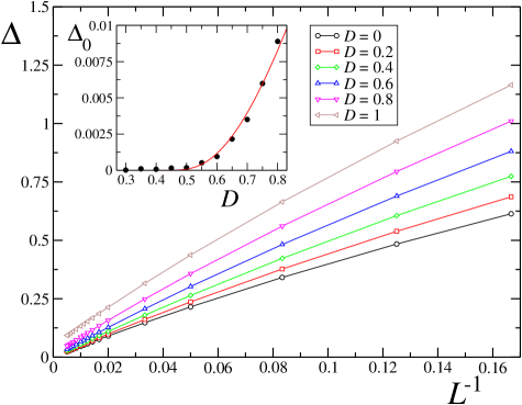
Figure 2: Ground state excitation energy $\Delta$ in the zero magnetization sector as a function of the inverse system size $L^{-1}$ (we show data ranging from $L=6$ to $L=200$). The various curves are for different values of the single-ion anisotropy $D$. In the inset we plot the asymptotic value $\Delta_{0}$ in the thermodynamic limit, as extracted from a quadratic fit of the data in main panel for $L\geq 50$ (black circles); the red line displays a fit $\Delta_{0}\propto\exp(-c/\sqrt{D-0.44})$ of data with $c\approx 2.977$.

As shown in figure 2, in the critical region $D<D_{c}$ the dynamical gap $\Delta$ scales approximately linearly as a function of the inverse system size $L^{-1}$. The same behavior also holds for relatively small values of $D-D_{c}$ within the gapped phase, as those considered in figure 2, so that the correlation length is still larger than the size of the system, and a quasi-critical regime is found [42]. On the other hand, we numerically checked that the leading term in finite-size corrections scale as $L^{-2}$ for $D\gtrsim 2$, when the system is far from criticality. We extrapolated the value of $\Delta_{0}=\Delta(L\to\infty)$ in the thermodynamic limit by performing a fit of numerical data for $L\geq 50$ which includes both the leading linear behavior and smaller quadratic corrections. Results are plotted in the inset of figure 2, as a function of $D$. According to the phase diagram of the system, which predicts a closure of the gap for $D<D_{c}\approx 0.44$, the asymptotic value of the gap is found to be constant and equal to zero for $0\leq D\lesssim 0.45$ (up to values $\sim 2\times 10^{-4}$), while it suddenly raises up as $\Delta_{0}\sim\exp(-c/\sqrt{D-D_{c}})$ in the gapped phase close to criticality. Thus the dynamical gap closes analogously to the gap between the ground state and the first excited state with unconstrained magnetization, which is called thermodynamical gap, in a BKT transition [44].

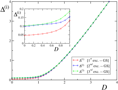
Figure 3: Excitation energy $\Delta^{(i)}$ of the three lowest excited dynamical levels for $L=100$ spins in the subspace $S^{z}_{\rm tot}=0$, as a function of $D$; the first excitation energy coincides with the dynamical gap: $\Delta^{(1)}\equiv\Delta$. The inset shows a zoom for $0\leq D\leq 1$ of the same plot.

The excitation energies of the first three dynamical excited levels in the subspace of zero magnetization and for a system of $L=100$ sites are displayed in figure 3, as a function of the anisotropy $D$. In the large-$D$ phase the dynamical gap $\Delta^{(1)}\equiv\Delta$ is well above the zero; when decreasing $D$ it closes approximately linearly until $D\sim 2$, then it continues closing as far as it approaches a region for $D\lesssim 0.5$, where it becomes almost constant and very small, as shown in the inset.

We point out that this type of behavior is quite different from the scenario elucidated in the spin-1/2 Heisenberg model of Ref. [22]. In that case two types of quenches involving the antiferromagnetic BKT isotropic point were considered. While in the second quenching scheme the system started from the critical region and advanced in the opposite direction with respect to our case, the first quench started from the antiferromagnetic region and crossed both the BKT point and the ferromagnetic isotropic point. Remarkably, the excess energy was found to be essentially characterized by the features of the ferromagnetic critical point, where the gap closes faster than in all the other points along the critical line. Therefore it was possible to identify a dominant critical point which allowed for the applicability of a LZ scaling argument in determining the defect density. On the other hand, our quench involves the BKT transition line close to the antiferromagnetic isotropic point, and there are no dominant critical points, thus leading to a more complex scenario, as explained in the following.

4.2 Oscillations in the excess energy for slow quenches

Let us first consider systems of small sizes, as shown in figure 4 for $L=6$ and $L=8$ sites. We have evaluated the excess energy both with the t-DMRG algorithm (filled circles), and with an exact diagonalization which does not truncate the system’s Hilbert space (empty squares). As the figure shows, data agree well.

On increasing the rate $\tau$, we can recognize two different regimes. For very small values of $\tau$ the excess energy is close to its maximum, and the dependence on the size and on $\tau$ is very small. These points correspond to very fast quenches, where the system dynamics is strongly non-adiabatic and the initial state is substantially frozen. As a consequence, the state after the quench is found to be in a superposition of many excited states of the final Hamiltonian. A second region is characterized by a dominant power-law decay, according to $E_{\rm exc}\sim\tau^{-2}$ (see the straight lines in the two insets of figure 4), that is superimposed to an oscillatory behavior. This can be explained within a LZ approximation: for small values of $D$ and $L$ the gap is large and proportional to $1/L$, therefore at very small sizes only the ground state and the first excited state participate to the evolution of the system, while all the other excited states are not accessible. The power-law decay, as well as the oscillations naturally arise when effects of finite duration time are taken into account [45]. Following the closing of the gap, the frequency of the oscillations decreases at increasing sizes, as it can be seen in the figure. The red curve displays a fit of numerical data obtained by an effective LZ model in which the initial coupling time $t_{i}<0$ is finite, and the final time is $t_{f}=0$ (see A for details on the fitting formula).

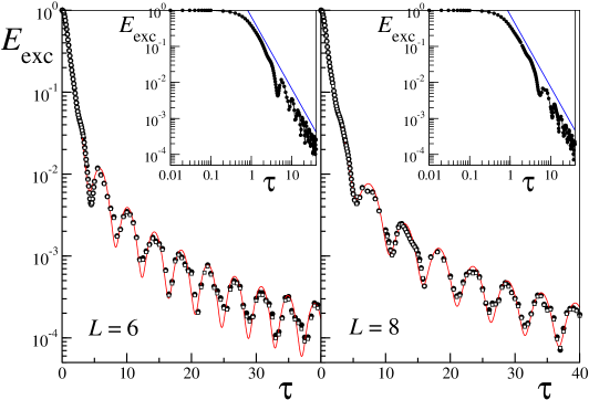
Figure 4: Final excess energy after an adiabatic quench of $D$ from $D_{\rm in}=1$ to $D_{\rm fin}=0$, as a function of the quench velocity $\tau$. Filled circles denote t-DMRG data, empty squares are obtained with exact diagonalization, while the continuous line is a numerical fit with the formula predicted by a LZ model for finite initial and final coupling times. The left panel shows data for $L=6$ sites, while the right one is for $L=8$. The insets show the same data in a log-log scale (straight blue lines denote a $\sim\tau^{-2}$ behavior). Note the smaller frequency of the oscillations for $L=8$.

The oscillatory behavior can be drastically suppressed starting from a larger value of $D_{\rm in}$, which corresponds, in the LZ model, to decreasing the initial coupling time $t_{i}$; for $t_{f}\leq 0$ and in the limit of $t_{i}\to-\infty$ the oscillations disappear and a pure power-law $\sim\tau^{-2}$ decay survives [45]. This is seen to emerge from numerical data of figure 5, where we started quenching from $D_{\rm in}=4$. Notice also the substantial independence of $E_{\rm exc}$ on the system size in the fast quenching limit.

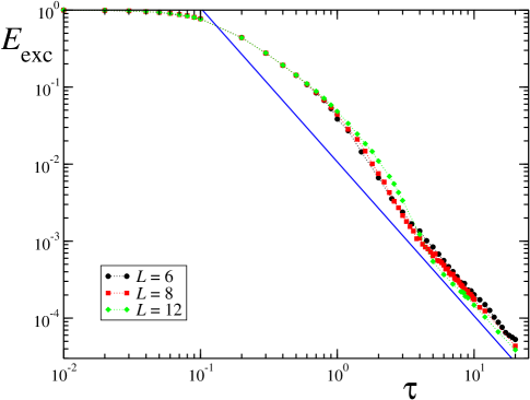
Figure 5: Excess energy after an adiabatic quench of $D$ from $D_{\rm in}=4$ to $D_{\rm fin}=0$, as a function of $\tau$. The various data are for different system sizes $L=6$ (black circles), 8 (red squares), 12 (green diamonds). The straight blue line indicates a behavior $E_{\rm exc}\sim\tau^{-2}$ and is plotted as a guideline.

4.3 Scaling regime

The analysis of the effects of the quantum phase transitions on the adiabatic quench dynamics demands sufficiently large system sizes. We now concentrate on this aspect and study the excess energy as a function of $\tau$ for considerably larger values of $L$. Due to the increasing computational difficulty in simulating large systems, we restrict ourselves to quenching schemes in which $D_{\rm in}=1$.

In figure 6 we plot the final excess energy of the system after a quench from $D_{\rm in}=1$ to $D_{\rm fin}=0$ of time duration $\tau$. Starting from fast quenches and going towards slower ones, we can now distinguish three different regimes: the first strongly non-adiabatic regime at small $\tau$ is analogous to the one previously discussed for small sizes. In the opposite limit of very slow quenches $\tau\gg 1$, we also recover the power-law $\tau^{-2}$ behavior superimposed to oscillations coming from an effective LZ description with finite coupling duration. Most interestingly, in between these two opposite situations, a characteristic power-law regime emerges, where:

$$E_{\rm exc}\sim\tau^{-\alpha}\,\quad{\rm with}\;\;\alpha\in[1,2]\,.$$ (6)

This is dominated by transitions to the lowest dynamically accessible gap, and it is crucially affected by the critical properties of the system. The crossover time $\tau^{*}$ at which this regime ends typically increases with the size, as it can be qualitatively seen from the figure (arrows denote a rough estimate of $\tau^{*}$ for the different sizes), and diverges in the thermodynamic limit; unfortunately we were not able to analyze the scaling with $L$, because of the intrinsic difficulty in estimating the ending point of the $\tau^{-\alpha}$ behavior. Nonetheless, even at asymptotically small quenching velocities, for very large sizes the scaling of defects (6) ruled by criticality persists, thus meaning that the system dynamics cannot be strictly adiabatic.

Figure 6: Final excess energy as a function of the quench rate $\tau$. The various panels stand for different system sizes. Symbols denote numerical t-DMRG data, while the straight line is a power-law fit that has been performed for $\tau<\tau^{*}$ ($\tau^{*}$ is indicated by the vertical arrow). The two straight dashed lines in the upper panels denote a $\tau^{-2}$ behavior, and are plotted as guidelines. The oscillating dashed line at $L=10$ is a fit of data with big $\tau$, according to the LZ model for a finite coupling duration. The values of $\alpha$ corresponding to the power-law fits are quoted in each panel. Here we set $D_{\rm in}=1$ and $D_{\rm fin}=0$.

The scaling of the decay rate $\alpha$ with the size has been analyzed numerically, for data corresponding to $L$ ranging from $10$ to $60$ spins; at $L<10$ this regime was not identifiable. Some representative cases are shown in figure 6, where each of the four panels stands for a given system size, while straight continuous lines indicate the best power-law fits of the scaling regions. In the case of $L=10$ sites (upper left panel), we cannot give a reliable estimate of $\alpha$, since the width of the scaling region is narrow and the fit is very sensitive to its actual starting and ending points. The straight line in the plot corresponds to $\alpha\approx 1.798$ and has been obtained from a power-law fit of numerical data from $\tau=1$ to $\tau^{*}=3$. As one can see, this is hardly distinguishable from the $\tau^{-2}$ power-law behavior of the slow-quench regime (straight dashed line), thus meaning that the existence of the scaling region itself is here in doubt. This is not the case for the other panels, where a power-law behavior of the type in equation (6) is clearly visible. Namely, we fitted our data until the $\tau^{*}$ value, that is labeled in figure 6 by a vertical arrow: as we could expect, the size of the scaling region increases with $L$.

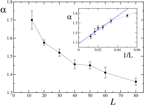
Figure 7: Power-law decay rate $\alpha$ in the intermediate scaling region for the excess energy, as a function of the system size $L$. The quench is performed from $D_{\rm in}=1$ to $D_{\rm fin}=0$. In the inset we plot the same quantity as a function of $1/L$. The blue line is a linear fit of data with $L\geq 30$, and predicts an asymptotic value of $\alpha_{\infty}\approx 1.28$ in the thermodynamic limit.

Summarizing the results obtained for the various sizes, in figure 7 we report the behavior of $\alpha$ as a function of $L$ (in the inset we plot the same data with $1/L$ on the $x$-axis). The uncertainty affecting the value of $\alpha$ extracted from the power-law fits of numerical t-DMRG data is mostly due to the inaccurate knowledge of the extremes of the scaling region. For each value of $L$, we identified a trial power-law region and then computed several values of $\alpha$ by progressively sweeping out the points from that region, starting from the borders. We then evaluated error bars, that are displayed in the plot, by performing a statistical analysis of the values of $\alpha$ thus obtained. In order to give an estimate of the power-law decay rate in the thermodynamic limit, we supposed that, at large $L$, $\alpha$ scales inversely proportional with the system size. In this way, performing a linear fit of data with $L\geq 30$, we extracted the asymptotic value $\alpha_{\infty}\approx 1.28$ in the thermodynamic limit (see straight blue line in the inset).

We would like to stress that, in this context, our numerical results seem not to find a straightforward explanation with LZ or KZ arguments. One could, for example, try to follow a standard LZ argument, that is based on the assumptions that the dynamical gap scales linearly with the inverse size, nearby and inside the critical region, and that the adiabaticity loss is essentially due to the presence of a dominant critical point, where the gap closes faster than elsewhere [11, 22]. In the LZ approximation, the probability of exciting the ground state is a global function of the product $\tau\Delta_{\rm m}^{2}$, where $\Delta_{\rm m}$ is the minimum gap achieved by the system during the quench. Assuming a critical scaling of the gap $\Delta_{\rm m}\sim L^{-1}$, as shown in figure 2, the density of defects can be estimated by evaluating the typical length $L_{\varepsilon}$ of a defect-free region, once the probability for this to occur is $\varepsilon$. As a consequence, this would give $E_{\rm exc}\sim 1/L_{\varepsilon}\propto\tau^{-1/2}$, exactly as in the Ising case, in contrast with numerical evidence. On the other hand, a scaling argument based on the KZ mechanism can be adopted [11, 12]; this relies on the fact that the dynamical gap $\Delta_{0}$ seems to close with $D-D_{C}$ as the thermodynamical gap in a BKT transition, that is, it depends on the anisotropy parameter as $\Delta_{0}\propto\exp(-c/\sqrt{D-D_{C}})$ [44], so that the critical exponent for the correlation length $\nu$ diverges. In this case, the KZ scaling argument predicts a power-law scaling exponent $\alpha=(d+z)\nu/(z\nu+1)$, $d$ being the dimension of the system and $z,\nu$ critical exponents; in our specific case $d=z=1,\nu\to\infty$ thus leading to $\alpha=2$ (plus some logarithmic corrections) [12, 17]. This again contrasts with our numerical evidence, thus revealing that the presence of a critical line in which the gap closes always in the same way seems to indicate that all the low-lying excitation spectrum becomes necessary to predict the actual behavior. We notice that the two above mentioned different dependencies of the dynamical gap on the inverse size, like $\sim 1/L$ for $L\to\infty$, and on the distance from the critical point, as $\sim e^{-c/\sqrt{D-D_{c}}}$, are confirmed quite precisely by our data.

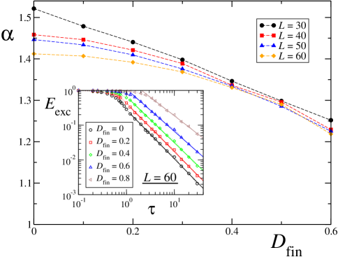
Figure 8: Power-law decay rate $\alpha$ as a function of the ending value for the quench $D_{\rm fin}<D_{\rm c}$ and for fixed $D_{\rm in}=1$. Data are for different system sizes, as explained in the caption. In the inset we display the excess energy for a quench ending at various $D_{\rm fin}$, and for a system size $L=60$. straight lines are power-law fits in the scaling regime.

We checked the dependence of $\alpha$ on the final point of the quench: in figure 8 we varied the ending point $D_{\rm fin}$, while keeping $D_{\rm in}$ and the system size fixed (explicit data for the excess energy $E_{\rm exc}$ as a function of $\tau$ are presented in the inset, at $L=60$). For values of $D_{\rm fin}$ outside the critical region we find that $\alpha$ depends on $D_{\rm fin}$ at finite sizes. Nevertheless, the range of the scaling region shrinks with $L$ and eventually disappears in the thermodynamic limit, so we argue that the dependence of $\alpha$ on $D_{\rm fin}>D_{\rm c}$ should be entirely due to finite size effects. For $D_{\rm fin}<D_{\rm c}$ we observe that the dependence of $\alpha$ on $D_{\rm fin}$ weakens as the system size is increased. In this case the scaling region is valid until a quench rate $\tau^{*}\stackrel{{\scriptstyle L\to\infty}}{{\longrightarrow}}+\infty$; the power-law decay rate tends to a value that is independent of $D_{\rm fin}<D_{c}$ and has been extrapolated from numerical data of figure 7 to be $\alpha_{\infty}\approx 1.28$.

5 Conclusions

In this work we have analyzed the quenched dynamics of a quantum anisotropic spin-1 XY chain, when it crosses a Berezinskii-Kosterlitz-Thouless quantum phase transition. The quench has been performed on the uniaxial single-spin anisotropy, and has been chosen to vary linearly in time with a given velocity. We focused on the residual excess energy of the system after the quench, and studied its dependence on the velocity of the quench. For very slow quenches and finite system sizes we were able to describe the properties of the system in terms of an effective Landau Zener model, where the system can only get excited to its first excited state. Most interestingly, we pointed out the emergence of an intermediate region where the excess energy drops as a power-law with the quench rate, and exhibits a non trivial scaling behavior. At least for the finite sizes considered here, the decay rate depends on the size of the crossed critical region, and cannot be explained in terms of usual scaling arguments, such as the standard Kibble-Zurek mechanism and its generalization to critical surfaces [22, 23, 24, 25]. In the thermodynamic limit the system obeys a non-trivial scaling behavior $E_{\rm exc}\sim\tau^{-\alpha}$, with $1<\alpha<2$, even when $\tau\to\infty$ (i.e., for very slow quenches).

Appendix A Landau-Zener model for finite coupling times

The Landau-Zener (LZ) model consists in a two level system describing an avoided level crossing: two energy levels moving in time are widely separated at first, then they approach each other with time, and finally part away again [31, 32]. When the two levels are well separated, each eigenstate preserves an individual character; on the other hand, when levels are close together, they mix due to their interaction. The Hamiltonian is given by:

$$\mathcal{H}_{LZ}=\left(\begin{array}[]{cc}-\Delta(t)&\Omega\\ \Omega&\Delta(t)\end{array}\right),$$ (7)

with a detuning $\Delta(t)=\beta^{2}t$ (where $\beta^{2}>0$), and a time independent coupling $\Omega$ that, in the original LZ model is supposed to last from $t_{i}=-\infty$ to $t_{f}=+\infty$ [31, 32]. Here we review the general case where the coupling is turned on at $t_{i}$ and off at $t_{f}$ [45]. The equation (7) is written in the basis of the two eigenstates of the Hamiltonian in absence of interaction.

The probability amplitudes $\vec{C}(t_{i})=[C_{1}(t_{i}),\,C_{2}(t_{i})]^{T}$ for the two levels at the beginning are connected to the ones at the final time $t_{f}$ by the unitary evolution matrix $U(t_{f},t_{i})$, so that: $\vec{C}(t_{f})=U(t_{f},t_{i})\,\vec{C}(t_{i})$. Their elements are given by:

$$U_{11}(T_{f},T_{i}) =\frac{\Gamma(1-\frac{1}{2}i\omega^{2})}{\sqrt{2\pi}}[D_{i\omega^{2}/2}(T_{f}\sqrt{2}e^{-i\pi/4})$$

$$\times D_{-1+i\omega^{2}/2}(T_{i}\sqrt{2}e^{i3\pi/4})+D_{i\omega^{2}/2}(T_{f}\sqrt{2}e^{i3\pi/4})$$

$$\times D_{-1+i\omega^{2}/2}(T_{i}\sqrt{2}e^{-i\pi/4})]\,,$$

$$U_{12}(T_{f},T_{i}) =\frac{\Gamma(1-\frac{1}{2}i\omega^{2})}{\omega\sqrt{\pi}}e^{i\pi/4}[-D_{i\omega^{2}/2}(T_{f}\sqrt{2}e^{-i\pi/4})$$

$$\times D_{i\omega^{2}/2}(T_{i}\sqrt{2}e^{i3\pi/4})$$

$$+D_{i\omega^{2}/2}(T_{f}\sqrt{2}e^{i3\pi/4})\,D_{i\omega^{2}/2}(T_{i}\sqrt{2}e^{-i\pi/4})]\,,$$

where we have introduced the rescaled time $T=\beta t$ and the scaled dimensionless coupling strength $\omega=\Omega/\beta$, while $D_{\nu}(z)$ denote the parabolic cylinder functions. If we suppose that the system is initialized in its ground state, i.e., $C_{1}(t_{i})=1,\;C_{2}(t_{i})=0$, the transition probability to the excited state at the final time is given by $P^{(d)}(t_{f},t_{i})=|U_{21}(t_{f},t_{i})|^{2}$.

This is related to the relevant adiabatic basis, that is the basis of the instantaneous system eigenstates, by a unitary transformation. If $\vec{A}(t)=[A_{1}(t),\,A_{2}(t)]^{T}$ are the probability amplitudes for the two levels in the adiabatic basis, then $\vec{A}(t)={\bf R}(t)\,\vec{C}(t)$, where ${\bf R}(t)$ is the rotation matrix

$${\bf R}(T)=\left(\begin{array}[]{cc}\cos\vartheta(t)&-\sin\vartheta(t)\\ \sin\vartheta(t)&\cos\vartheta(t)\end{array}\right),$$ (10)

with $\tan[2\vartheta(t)]=\Omega(t)/\Delta(t)$. Therefore, the evolution matrix in the adiabatic representation is given by $U_{a}(t_{f},t_{i})={\bf R}^{T}(t_{f})\,U(t_{f},t_{i})\,{\bf R}(t_{i})$, and the adiabatic-following solution for the transition probability is $P^{(a)}(t_{f},t_{i})=|U^{(a)}_{21}(t_{f},t_{i})|^{2}$.

For the original LZ model, where the coupling is supposed to last from $t_{i}\rightarrow-\infty$ to $t_{f}\rightarrow+\infty$, the expression for the excitation probability at the end of the quench in the adiabatic basis simplifies to an exponential form:

$$P^{(a)}(+\infty,-\infty)=e^{-\pi\omega^{2}}\,.$$ (11)

In the case of a finite coupling duration, that ends before or exactly at the crossing (i.e., $t_{f}\leq 0$), we have a much involved expression, which predicts a leading power-law behavior $P^{(a)}\sim\tau^{-2}$ superimposed to an oscillating behavior. Eventually oscillations are damped for long lasting couplings: in the limiting case where the quench ends at the critical point and is infinite lasting ($t_{i}=-\infty,\,t_{f}=0$), the probability is given by

$$P^{(a)}(0,-\infty)=\frac{1}{16\,\omega^{4}}\sim\frac{1}{\tau^{2}}\,.$$ (12)

The scaling with the quench velocity $\tau$ follows from the fact that the times $t\propto\tau$, while $\beta^{2}\propto 1/\tau$ (this implies that $\omega\propto\sqrt{\tau}$).

We used the explicit formula for the adiabatic transition probability $P^{(a)}(0,t_{i}<0)$ in order to fit t-DMRG data for the excess energy of our system in the regime of large $\tau$, where defects still do not form and the quench dynamics can be considered adiabatic. While it is clear that $t_{i}<0$ in our case, it is not obvious a priori whether $t_{f}<0$ or $t_{f}=0$, since LZ relies on the assumption that there is only one point of closest approach of the energy levels; on the contrary, in our model we have a whole critical line. We actually chose $t_{f}=0$ and used $t_{i}<0$ as a fitting parameter, having not a rigorous criterion at our disposal, but following the qualitative picture suggested from figure 3: the gap closes monotonically during the quench, reaching the minimum at $D_{\rm fin}$. The red curves in figure 4 have been obtained by fitting numerical data with the theoretical prediction given by $P^{(a)}$; we admitted a global rescaling prefactor $\phi$ and imposed the following constraints: $T_{i}=-T_{0}\sqrt{\tau}$, $T_{f}=0$, $\omega=\omega_{0}\sqrt{\tau}$. The fitting parameters are $T_{0},\,\omega_{0},\,\phi$. For the left panel ($N=6$) we chose $T_{0}\approx 0.8,\,\omega_{0}=0.84,\,\phi=1.72$, while for the right one ($N=8$) $T_{0}\approx 0.735,\,\omega_{0}=0.7,\,\phi=0.9$.

References

References

- [1] Bloch I, Dalibard J and Zwerger W, 2008 Rev. Mod. Phys. 80 885
- [2] Greiner M, Mandel O, Esslinger T, Hänsch T W and Bloch I, 2002 Nature 415 39
- [3] Orzel C, Tuchman A K, Fenselau M L, Yasuda M and Kasevich M A, 2001 Science 291 2386
- [4] Kinoshita T, Wenger T and Weiss D S, 2006 Nature 440 900
- [5] Iglói F and Rieger H, 2000 Phys. Rev. Lett. 85 3233; Sengupta K, Powell S and Sachdev S, 2004 Phys. Rev. A 69 053616; Calabrese P and Cardy J, 2006 Phys. Rev. Lett. 96 136801; Cazalilla M A, 2006 Phys. Rev. Lett. 97 156403; Rigol M, Dunjko V, Yurovsky V and Olshanii M, 2007 Phys. Rev. Lett. 98 050405; Kollath C, Läuchli A M and Altman E, 2007 Phys. Rev. Lett. 98 180601; Manmana S R, Wessel S, Noack R M and Muramatsu A, 2007 Phys. Rev. Lett. 98 210405; Cramer M, Dawson C M, Eisert J and Osborne T J, 2008 Phys. Rev. Lett. 100 030602; Barthel T and Schollwöck U, 2008 Phys. Rev. Lett. 100 100601; Eckstein M and Kollar M, 2008 Phys. Rev. Lett. 100 120404; Rossini D, Silva A, Mussardo G and Santoro G E, 2009 Phys. Rev. Lett. 102 127204
- [6] Fahri E, Goldstone J, Gutmann S, Lapan J, Lundgren A and Preda D, 2001 Science 292 472
- [7] Santoro G E, Martonak R, Tosatti E and Car R, 2002 Science 295 2427
- [8] Santoro G E and Tosatti E, 2006 J.Phys. A 39 R393
- [9] Kibble T W B, 1976 J. Phys. A 9 1387; 1980 Phys. Rep. 67 183
- [10] Zurek W H, 1985 Nature 317 505; 1993 Acta Phys. Pol. B 24 1301; 1996 Phys. Rep. 276, 177
- [11] Zurek W H, Dorner U and Zoller P, 2005 Phys. Rev. Lett. 95 105701
- [12] Polkovnikov A, 2005 Phys. Rev. B 72 161201(R)
- [13] Damski B, 2005 Phys. Rev. Lett. 95 035701
- [14] Dziarmaga J, 2005 Phys. Rev. Lett. 95 245701
- [15] Damski B and Zurek W H, 2006 Phys. Rev. A 73 063405
- [16] Cherng R W and Levitov L, 2006 Phys. Rev. A 73 043614
- [17] Cucchietti F M, Damski B, Dziarmaga J and Zurek W H, 2007 Phys. Rev. A 75 023603
- [18] Cincio L, Dziarmaga J, Rams M M and Zurek W H, 2007 Phys. Rev. A 75 052321
- [19] Caneva T, Fazio R and Santoro G E, 2007 Phys. Rev. B 76 144427
- [20] Caneva T, Fazio R and Santoro G E, 2008 Phys. Rev. B 78 104426
- [21] Patanè D, Silva A, Amico L, Fazio R and Santoro G E, 2008 Phys. Rev. Lett. 101 175701
- [22] Pellegrini F, Montangero S, Santoro G E and Fazio R, 2008 Phys. Rev. B 77 140404 (R)
- [23] Sengupta K, Sen D and Mondal S, 2008 Phys. Rev. Lett. 100 077204
- [24] Deng S, Ortiz G and Viola L, 2008 Europhys. Lett. 84 67008
- [25] Divakaran U, Dutta A and Sen D, 2008 Phys. Rev. B 78 144301
- [26] Sen D, Sengupta K and Mondal S, 2008 Phys. Rev. Lett. 101 016806
- [27] Cincio L, Dziarmaga J, Meisner J and Rams M M, 2009 Phys. Rev. B to appear Preprint arXiv:0812.1455 [quant-ph]
- [28] Polkovnikov A and Gritsev V, 2008 Nature Phys. 4 477
- [29] De Grandi C, Barankov R A and Polkovnikov A, Phys. Rev. Lett. 101, 230402 (2008).
- [30] Schützhold R, Uhlmann M, Xu Y and Fischer U R, 2006 Phys. Rev. Lett. 97 200601
- [31] Landau L D and Lifšits E M, 1958 Quantum Mechanics (New York: Pergamon)
- [32] Zener C, 1932 Proc. R. Soc. London A, 137 696
- [33] Schulz H J, 1986 Phys. Rev. B 34 6372
- [34] De Nijs M and Rommelse K, 1989 Phys. Rev. B 40 4709
- [35] Altman E and Auerbach A, 2002 Phys. Rev. Lett. 89 250404
- [36] Huber S D, Altman E, Büchler H P and Blatter G, 2007 Phys. Rev. B 75 085106
- [37] Clark S R and Jaksch D, 2004 Phys. Rev. A 70 043612
- [38] Fisher M P A, Weichman P B, Grinstein G and Fisher D S, 1989 Phys. Rev. B 40 546
- [39] Jaksch D, Bruder C, Cirac J I, Gardiner C W and Zoller P, 1998 Phys. Rev. Lett. 81 3108
- [40] Chen W, Hida K and Sanctuary B C, 2003 Phys. Rev. B 67 104401
- [41] Pires A S T and Gouvêa M E, 2005 Eur. Phys. J. B 44 169
- [42] Degli Esposti Boschi C, Ercolessi E, Ortolani F and Roncaglia M, 2003 Eur. Phys. J. B 35 465; Degli Esposti Boschi C and Ortolani F, 2004 Eur. Phys. J. B 41 503; Campos Venuti L, Degli Esposti Boschi C, Ercolessi E, Morandi G, Ortolani F, Pasini S and Roncaglia M, 2006 Eur. Phys. J. B 53 11
- [43] Schollwöck U, 2005 Rev. Mod. Phys. 77 259; De Chiara G, Rossini D, Rizzi M and Montangero S, 2008 J. Comp. Theor. Nanosci. 5 1277
- [44] Chaikin P M and Lubensky T C, 1995 Principles of Condensed Matter Physics (Cambridge: Cambridge University Press)
- [45] Vitanov N V and Garraway B M, 1996 Phys. Rev. A 53 4288; Vitanov N V, 1999 Phys. Rev. A 59 988