How to Track Protists in Three Dimensions

Abstract

We present an apparatus optimized for tracking swimming microorganisms in the size range $10-1000$ $\mu$m, in three dimensions (3D), far from surfaces, and with negligible background convective fluid motion. CCD cameras attached to two long working distance microscopes synchronously image the sample from two perpendicular directions, with narrowband dark-field or bright-field illumination chosen to avoid triggering a phototactic response. The images from the two cameras can be combined to yield 3D tracks of the organism. Using additional, highly directional broad-spectrum illumination with millisecond timing control the phototactic trajectories in 3D of organisms ranging from Chlamydomonas to Volvox can be studied in detail. Surface-mediated hydrodynamic interactions can also be investigated without convective interference. Minimal modifications to the apparatus allow for studies of chemotaxis and other taxes.

I Introduction

Protists, the grouping of eukaryotic microorganisms that encompasses such diverse entities as flagellated and ciliated protozoa protistology (e.g., Euglena, Paramecium) and motile green alga greenalgae (e.g., Chlamydomonas, Volvox – shown in Fig. 1), constitute an important class of organisms in the study of evolutionary biology, biological physics, and, recently, biological fluid dynamics multicellular ; flagflows ; Takuji_paramecium . Many flagellated protists display swimming behavior that is inherently three-dimensional (3D). A number of important questions in biology and physics are associated with how the motion of such organisms is related to their body plan and to external stimuli such as light Hill_phototaxis ; Schaller , dissolved molecular species, gravity, temperature, boundaries waltzing , and electromagnetic fields. It is thus desirable to track their position and orientation in 3D Vlad1 ; Vlad2 with high spatio-temporal resolution and, unless desired, free from systematic bias introduced by external stimuli, background fluid motion, and hydrodynamic surface effects surfeffect ; squires2001 .

The first apparatus able to track microorganisms in 3D was designed for bacteria berg1971 and utilized an analogue feedback loop that moved the microscope stage to keep a bacterium centered in the field of view. Larger microorganisms such as protists require larger sample chambers, reaching millimeters or even centimeters in depth to avoid boundary-induced hydrodynamic effects. In this regime, methods based on a moving microscope stage are not suitable, as they induce uncontrolled background fluid motion in the sample chamber. Similar considerations enter the study of the millimetric nematode C. elegans crawling on the surface of agar, for which a moving substrate introduces unwanted mechanical stimuli. Instead, the camera itself can by moved by motors controlled by an algorithm that dynamically centers the worm in the field of view ryu . Several apparati for tracking the 3D motion of microscopic particles without a moving stage have emerged in recent years, yet none is ideal for studying the swimming of protists. Methods based on controlled defocussing of particles wu2005 ; willert1992 , placing a cylindrical lens in the imaging optics of the microscope kao1994 , or measuring the deflections of a laser beam that is focused close to a particle peters1998 ; ghislain1994 all suffer from a small tracking range along the optical axis. Observing a sample which is illuminated from the side with a continuous gradient of color in order to color-code the third dimension matsushita2004 ; mcgregor2008 suffers from low spatial resolution in that dimension, and may provide a photostimulus to protists. Tracking objects with a confocal microscope is only possible when the objects move at very low speeds dinsmore2001 ; rabut2004 . Digital in-line holography may also be used for 3D particle tracking, yet even vibrations with amplitudes $<1$ $\mu$m of components along the optical path lead to a time-varying background in the hologram that can significantly degrade the signal of the moving object.

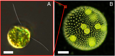
Figure 1: Two protists whose swimming motion is of interest in this work. (A) Chlamydomonas reinhardtii (scale bar $5$ $\mu$m) and (B) Volvox carteri (scale bar $200$ $\mu$m).

The difficulties mentioned above can be overcome by using more than one camera to observe synchronously the sample chamber from different angles and then combining the images to yield 3D tracks of particles. Yet, existing implementations of this technique can not be easily adapted to track microscopic objects maas1993 ; hoyer2005 ; they either have a controlled but undesirable shear flow grillet2007 , have not integrated any control of thermal convection strickler1998 , or have been implemented with a temperature gradient across the sample ($\sim 3$ K/cm) to eliminate thermal convection thar2000 . The latter method is an important advance, but may introduce an unwanted behavioral stimulus to protists.

Here we present an apparatus that uses two identical imaging assemblies at right angles to each other that can be used in dark- and bright-field illumination, combined with systems to deliver photo-stimuli, to control temperature inside the sample, and to eliminate background fluid motion in large sample chambers (up to $2.5\times 2.5\times 5$ cm) filled with aqueous growth medium, by homogenizing the temperature inside the sample chamber to millikelvin precision. The apparatus uses almost entirely off-the-shelf components and requires minimal expertise in optics. Online supporting material includes software to control the hardware and to perform 3D tracking. We discuss the resolution and limitations of the apparatus, present swimming trajectories of the protists Chlamydomonas and Volvox in 3D, and illustrate with dual-view particle imaging velocimetry (PIV) the flow field that Volvox generates near a surface.

II Experimental Apparatus

The 3D tracking system, shown schematically in Fig. 2, is based on a flexible but powerful imaging system, phototactic stimulus lights, and equipment to control and homogenize the temperature inside the sample chamber. These three elements are now explained in detail.

The imaging system is comprised of two identical assemblies that are mounted at right angles on a vibration isolation table (Science Desk, with $900\times 1200\times 60$ mm breadboard, Thorlabs, Ely, UK). A monochrome FireWire CCD camera (Pike F145B, Allied Vision Technologies, Stadtroda, Germany; $1388\times 1038$ pixels, each $6.45\times 6.45$ $\mu$m, maximal frame rate of $30$ fps, and support for external triggering) was attached to each of the two microscopes (InfiniVar CFM-2/S, Infinity Photo-Optical, Boulder, CO). These are continuously focusable with a working distance between $18$ mm and $\infty$, yielding a maximum magnification of $\times 9$ at the smallest available working distance. To allow a variable working distance, the camera/microscope assemblies were mounted on sliding rails (PRL-12, Newport Corp., Irvine, CA) via standard post/post support hardware. The horizontal rail was attached directly to the breadboard while the vertical one was attached to a movable and lockable rail carrier on a large optical rail (X95, Newport Corp.) mounted vertically to the optical breadboard. The outer chamber (see Fig. 2, and details below) limits the smallest working distance to $\sim 60$ mm, yielding a magnification of $\times$1. While sufficient to image protists of size $\sim 10$ $\mu$m with dark-field illumination, such organisms are better visualized with an additional $\times 2$ magnifier lens (2xDL, Infinity Photo-Optical). This increases the working distance and the depth of field, as discussed below.

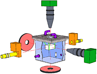
Figure 2: Schematic drawing of apparatus. The outer chamber (light blue, lid and flange in grey) contains a water bath, fed through inlets and outlets (purple), and mixed with a magnetic stir bar (white) driven by a motor external to the tank (not shown). The sample chamber (white) is suspended by stainless steel holders (light green), and illuminated by annular LED arrays (red). Microorganisms are visualized with two long-working-distance microscopes (dark gray) equipped with CCD cameras (dark green). Phototactic stimulus is provided by two LED and lens assemblies (yellow), and controlled by shutters (orange).

The imaging system can be used with dark- or bright-field illumination: bright-field can be advantageous for organisms larger than $\sim 100$ $\mu$m as it captures more details of the organism (e.g., the body axis); dark-field can be desirable when the organism is so small that only center-tracking is possible, as under these conditions it yields a better signal-to-noise ratio. The flexibility to use both illumination techniques is obtained by using an annular LED array (LFR-100-R, CCS Inc., Kyoto, Japan) as the (unpolarized) light source for each microscope. Dark-field illumination is achieved when the field of view of the microscope only includes the dark region in the center of the LED annulus. Bright-field illumination is achieved by inserting a diffuser plate (bulk frosted acrylic cut to size, RS components, UK) in between the LED array and the outer chamber, as far from the LED array as possible. We chose the color of the LED array to be narrowband red ($655$ nm, $21$ nm bandwidth) as it has been shown that this color does not trigger a phototactic response in motile green algae volvox_actionspectrum1 .

For phototaxis studies, two opposing light sources are required in order to observe reproducible light-induced U-turns. The photo-stimulus lights were two broad spectrum cool white Luxeon LEDs (MWLED, Thorlabs), collimated with a short focal length lens ($f=35$ mm, LA1027, Thorlabs), and mounted to a shutter with millisecond precision (SH05, Thorlabs). The shutter/LED assemblies are mounted via standard cage hardware (Thorlabs) to posts on rotating stages (RP01, Thorlabs), allowing the direction of the light to be controlled. The stimulus direction was typically chosen to be horizontal in order to avoid an additional gravitational stimulus. This choice forces the common axis of the two cameras to be horizontal, along the stimulus direction. The beam diameter was controlled with an iris (SM1D12, Thorlabs) to illuminate only those faces of the sample chamber perpendicular to the common axis of the two cameras, thereby avoiding reflections, and the resulting unclear stimuli, from the other four faces.

The two CCD cameras and shutters for the photo-stimulus lights were controlled with labview including the add-on toolbox ni-imaq for 1394-ieee cameras (National Instruments, Austin, TX), allowing precise synchronization of image acquisition. A labview program is part of the supporting online material.

In order to combine the images from both cameras to yield 3D swimming tracks, it is crucial that both microscopes operate at the same magnification (i.e. the same working distance). This is easily achieved to sufficient precision by replacing the sample chamber with a tilted calibration ruler that is observable through both cameras, and adjusting the working distance until the field of view of both cameras has the same physical size. After this calibration step, the microscopes need to be aligned along their common axis such that the field of view of both cameras contains the same section of the common axis. This axis alignment greatly improves the ability to reconstruct 3D tracks, as explained in Section III.

To obtain swimming trajectories that are not influenced by hydrodynamic surface effects or background flows, it is desirable to have a sample chamber that is as large as possible, while maintaining the fluid within it perfectly still. A stationary fluid can only be obtained if the temperature in the chamber and of the chamber walls is very homogeneous, thereby eliminating thermal convection caused by heating from the two LED arrays (each LED array consumes $\sim 3.6$ W). For a closed chamber, the critical Rayleigh number above which thermal convection starts to occur is $Ra_{\rm c}=\alpha gL^{3}\Delta T/\nu\kappa\simeq 1708$, where $\alpha$ is the thermal expansion coefficient of the fluid, $g$ is the gravitational acceleration, $\kappa$ is the thermal diffusivity, $\nu$ is the kinematic viscosity, and $L$ is the length scale across which there is a temperature difference $\Delta T$ criticalRayleigh . While the precise value of $Ra_{\rm c}$ depends on the geometry of forcing and on boundary conditions, the scale of temperature differences involved for water ($\alpha=2\times 10^{-4}$ K^-1, $\kappa=1.4\times 10^{-3}$ cm²/s, $\nu=0.01$ cm²/s) is roughly $100$ mK for a one centimeter length. The largest chambers that have previously been temperature-homogenized below the thermal convection threshold, under comparable conditions to those presented here, have $L\sim 1$ cm in sedimentation studies segre1997 ; weitzNbody . The system presented here eliminates thermal convection in chambers as large as $2.5\times 2.5\times 5$ cm, implying temperature differences between faces of the chamber to be below $\sim 8$ mK.

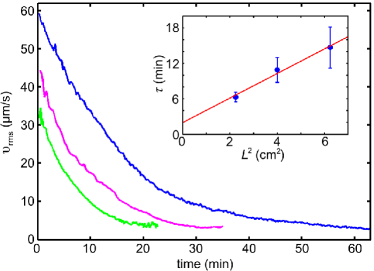
Figure 3: Decay of convective motion in the inner sample chamber. Curves show the root-mean-squared velocity $v_{\rm rms}$ within the chamber, obtained by PIV, as a function of time for three different chamber dimensions: blue - $2.5\times 2.5\times 2.5$ cm, magenta - $2.0\times 2.0\times 2.0$ cm, green - $1.5\times 1.5\times 1.5$ cm. Inset shows the time constant for each decay as a function of chamber size, consistent with the $L^{2}$ diffusive scaling.

Recognizing that in Stokes flow the effects of boundaries at a distance $h$ from compact objects acted upon by gravity fall off as $h^{-1}$, and given that swimming trajectories can easily sample a vertical scale that is $5$ times the organism diameter, the sample chamber should be $>20$ times the organism diameter for surface effects to remain below the 5% level surfeffect ; squires2001 . A chamber of this size thus allows protists as large as $1000$ $\mu$m to be studied with negligible hydrodynamic surface effects.

Before explaining how the temperature in the sample chamber is controlled and homogenized, it is necessary to give details of the outer and sample chambers. The outer chamber has dimensions $12\times 12\times 10$ cm, two inlets and two outlets (as shown in Fig. 2) and is made from $2.75$ mm thick borosilicate glass (custom made by Fine Glass Finishers Ltd., Great Chesterford, UK). The flange and lid of the outer chamber were custom made out of PVC with a CNC machine. The three types of sample chamber used were (i) custom cuvettes made from standard microscope slides cut with a tungsten glass scriber (LAC-450-A, Fisher Scientific, UK) and glued together with UV-curing optical glue (NOA68, Norland Products, Cranbury, NJ), cured in a UV Chamber (ELC-500, Electro-Lite Corporation, Bethel, CT), (ii) non-standard commercial glass cuvettes (VitroCom, Mountain Lakes, NJ), and (iii) standard glass cuvettes. The sample chamber is held rigidly in the center of the outer chamber by four thin stainless steel rods ($1.6$ mm diameter). Each rod was inserted into a corresponding tight-fitting hole in the lid and fixed with a set screw, allowing easy modification of the holding arrangements for the different chambers.

It is well-known that the flagella of protists such as Chlamydomonas have a strong tendency to stick to glass surfaces flagella_sticking . As cells swim around the chamber they inevitably collide with the chamber walls. To avoid any problem with sticking, the glass is coated with PDMS (Sylgard $184$, Dow-Corning, Belgium) and etched for $3$ minutes in a plasma cleaner (Femto, Diener Electronic, Nagold, Germany), following a published protocol whitesides .

The temperature in the sample chamber is controlled by cycling filtered water through the outer chamber from a large tank that contains a submersed thermostatic heater (Jäger Eheim, Deizisau, Germany) and pump (Eheim, Deizisau, Germany). In order to homogenize the temperature in the sample chamber, the pump is switched off, and strong rare earth magnets (EP200, e-Magnets UK) are spun at $\sim 300$ rpm by a sturdy motor (178-5112, RS components, UK) on the outside of the outer chamber, thereby moving a Teflon-coated $5$ cm magnetic stir bar inside the outer chamber at the same speed. This stirring evens out the temperature within the outer chamber and, if the stir bar is spun at the appropriate speed and place in the outer chamber, moves the water past the faces of the sample chamber without setting up recirculating vortices on the faces. By injecting inexpensive tracer particles (size $\leq$75 $\mu$m, Pliolite VTAC-L, Eliokem, Villejust, France) into the outer chamber in order to visualize the flow across the faces of the sample chamber, we found that the arrangement drawn in Fig. 2 can homogenize the temperature inside the sample chamber below the threshold $Ra_{\rm c}$.

The flows within the sample chamber were quantified with commercial PIV software (FlowManager, Dantec Dynamics, Skovlunde, Denmark). As a metric for the extent of flows throughout the chamber, we report the r.m.s. velocity $v_{\rm rms}$ obtained by uniform averaging over the field of view of one camera. Figure 3 shows that $v_{\rm rms}$ decays exponentially as a function of time after the stirring of the water bath has begun, with a time constant $\tau(L)$ that depends on the smaller chamber dimension $L$. It is straightforward to see when the temperature difference falls below the threshold for convection, as tracer particles that are used to visualize the convective flow in the sample chamber will suddenly begin to fall out of the fluid at approximately their Stokes sedimentation speed, forming a sedimentation front that propagates downward. For $10$ $\mu$m latex beads (C37259, Invitrogen, Carlsbad, CA), the Stokes sedimentation speed is $\sim 3$ $\mu$m/s. This serves as a lower bound for $v_{\rm rms}$ in Fig. 3. We expect $\tau(L)$ to arise from viscous dissipation, and thus to scale as $\tau(L)\sim L^{2}/\nu$. In water this yields times on the order of a few to ten minutes for $L$ in the range $1-2.5$ cm, consistent with the data in Fig. 3. Each curve conforms well to a single exponential decay, and the fitted times $\tau(L)$ obey well the expected quadratic scaling as shown in the inset to Fig. 3, with a value not far from that expected from the kinematic viscosity of water.

III Tracking Software

The 3D tracking was done by analyzing the image sequences from each camera separately, giving a set of two two-dimensional (2D) tracks, and combining suitable tracks from these two sets to yield 3D trajectories.

Modified matlab (MathWorks, Natick, MA) versions of freely available eric_weeks_web particle tracking routines written by J.C. Crocker and D.G. Grier were used for the 2D tracking, allowing many organisms to be tracked at the same time. To track organisms that are so small that they appear circular and without internal structure in dark-field images (e.g., Chlamydomonas), no modifications to the original versions of the code need to be made. To track extended objects (e.g., Volvox) the routines that identify the center of the object need to be modified in a way that depends on the shape and structure of the object. For bright-field images of the spherical Volvox, all internal structure of Volvox was removed by histogram equalization, followed by spatial band pass filtering. The resulting image was then convolved with a binary disk-shaped kernel, yielding an image in which the centroids of peaks correspond to the Volvox centers in the original image. A Volvox colony carries daughter colonies inside it (see Fig. 1), which are fixed in the posterior hemisphere and therefore act as convenient markers of the body axis. The axis of Volvox can thus be determined by finding the vector between the geometric center of Volvox and the center of brightness of the daughter colonies inside Volvox for both directions and then combining these two vectors to obtain a 3D axis. The modified code also allows additional information for each Volvox to be gathered, such as the orientation of the body axis.

To identify two 2D tracks that are suitable for synthesizing into a 3D track, the two sets of 2D tracks were compared along the common axis of the field of view of the two cameras. Consider one of the possible combinations of two 2D tracks. Even if these two tracks are projections of positions of a single organism, the tracks usually do not completely overlap in time, because during the course of a long track the signal from the tracked object may fall below the tracking threshold so that the object ‘drops out’ of the tracking data xu2008 . This means that only the time-overlapping sections of each track can be compared. Because of the precise alignment of the field of view of both cameras (see Sec. II), a decision upon whether the two 2D tracks are from the same organism can be made by finding the r.m.s. difference between the position-coordinate along the common axis. The two 2D tracks for which this value is minimal (and below a certain threshold) are then synthesized into a 3D trajectory. Code that can perform all the operations described above is part of the supporting online material.

IV Performance

The tracking precision of the apparatus has been determined by the standard method gelles ; cheezum of observing fluctuations in the tracked position of particles that are fixed between two cover slips. The precision was tested at the minimum working distance the apparatus allows (60 mm, corresponding to $\times$1 magnification), for two different types of objects. For monodisperse 10 $\mu$m latex beads imaged in dark-field illumination, the uncertainty in the position was found to be $\leq 1.5$ $\mu$m, if the $\times$2 magnifier lens is mounted to the microscope. For objects in the size range 425-500 $\mu$m (Volvox fixed with iodine), in bright-field illumination, the uncertainty was found to be $\leq 1.3$ $\mu$m without the magnifier lens.

The performance of the apparatus is determined not only by the uncertainty in spatial position, but also by the overall volume in which 3D tracking can be performed. This volume is set by the depth of field of the microscope. For the purpose of simply tracking the center of a spherical object, the object can be out of focus as long as the signal in the image intensity profile is sufficiently large. Therefore the “trackable depth” (TD), which we define as the depth in which the signal/noise $\leq 4$, is a more suitable measure for the trackable volume than the depth of field. The TD is strongly dependent on the object size and on the signal (dark-field illumination gives a larger signal). We measured the TD for 10 $\mu$m beads in dark-field to be $5.8$ mm ($11.9$ mm) at a working distance of $60$ mm ($100$ mm). Imaged in bright-field, fixed Volvox of size 425-500 $\mu$m have TD $=18.3$ mm at the minimum working distance of $60$ mm.

A limitation of the tracking software presented here is that the concentration of organisms in the sample chamber should not be so large that swimmers overlap frequently in the 2D images from each camera. As the tracking software can not distinguish overlapping objects, a high concentration of swimmers would result in very short 2D tracks, and therefore less accurate synthesizing of 2D tracks to a 3D track. An alternative method for obtaining 3D tracks from the images of more than one camera is to determine the 3D position of every particle at every time point. This approach is often taken in 3D Lagrangian particle tracking maas1993 ; kieft2002 , and can handle larger concentrations of trackable objects, but is usually implemented with at least three cameras in order to reduce frequent ambiguities in the 3D particle identification, and requires an elaborate calibration. This 3D tracking method could be implemented with the apparatus described here, if one of the stimulus lights is replaced by a third microscope-camera-assembly.

Another limitation is the size of the outer chamber, which limits the magnification to values that are not sufficient for tracking small bacteria (e.g., E. coli), even though the microscope has a maximum magnification of $\times$18 (including the $\times$2 magnifier lens). For tracking bacteria sample chambers of size $2\times 2\times 2$ mm berg1972 may be used, for which the temperature-homogenizing outer chamber is not needed.

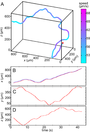
Figure 4: Reconstruction of a swimming trajectory of Chlamydomonas reinhardtii. Gravity is along negative $z$-direction. (A) 3D trajectory, color-coded to indicate local speed. Red dot indicates start of the trajectory. (B)-(D) Three components of position versus time. In (B) are the two traces $x(t)$ from the two cameras.

V Application of apparatus to track Chlamydomonas and Volvox

The apparatus was tested on two low-Reynolds number swimmers of very different size: Chlamydomonas reinhardtii (diameter of $\sim 10$ $\mu$m) and Volvox barberi (diameter of $\sim 600$ $\mu$m). Both species were grown axenically in Standard Volvox Medium (SVM) svm with sterile air bubbling, in diurnal growth chambers (Binder KBW400, Tuttlingen, Germany) set to a daily cycle of $16$ h in cool white light ($\sim 4000$ lux) at $28^{\circ}$ C and $8$ h in the dark at $26^{\circ}$ C. Sample chambers were filled with SVM and were of size $2.5\times 2.5\times 5$ cm for Volvox, and $1\times 1\times 4$ cm (standard cuvette) for Chlamydomonas.

The biflagellated Chlamydomonas beats its flagella at $\sim 40$ Hz, primarily in the manner of the breast stroke. Its most familiar swimming trajectory is helical, with a radius of $20$ $\mu$m and a speed on the order of $50$ $\mu$m/s. The cell has an “eye-spot” that serves as a photosensor, and the changing illumination levels of the eye-spot lead to transient changes in flagellar beat dynamics in such a manner that the cell can turn toward the light.

Figure 4A shows a $45$ s trajectory, obtained without phototactic stimulus, during which the cell explored a volume less than $1$ mm³. The manner in which the two 2D trajectories from the cameras are synthesized into a 3D trajectory is indicated in panels (B)-(D) of the figure. The $x$-axis is common to the two cameras, and the overlap between the two is clear in Fig. 4B. The very slight graded mismatch between the two $x$-component curves reflects a slight misalignment of the cameras, and is easily removed by remapping the pixel coordinates.

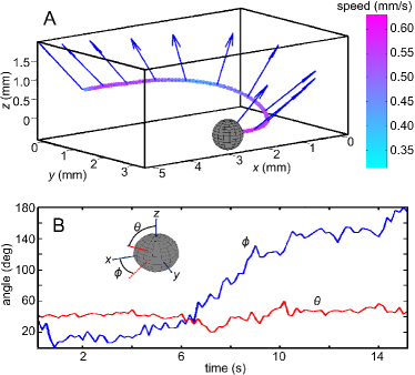
Figure 5: A phototactic turn of Volvox barberi. (A) The positional and orientational measurements are illustrated by vectors indicating the body axis, and swimming-speed-dependent coloration of the track. To initiate the 180^∘ change swimming direction, the light initially was from the right along the $x$-axis and then changed to come from the left. Gravity is directed along the negative $z$-direction. Sphere represents initial position along the track. (B) Evolution of the body axis during the phototactic turn is described in terms of two angles $\theta$ and $\phi$.

Volvox barberi typically has $10,000-50,000$ biflagellated somatic cells rigidly embedded at the surface of a transparent extracellular matrix. These beat at a typical frequency of $20$ Hz, primarily from the anterior pole to the posterior pole, with a slight tilt of the beat plane which leads to the characteristic spinning motion as it swims at speeds up to $800$ $\mu$m/s solari_barberi . Just as in Chlamydomonas, each somatic cell has an eye-spot that modulates the beating of its two flagella, allowing the whole colony to perform phototaxis. A 3D track of the Volvox center and body axis during a phototactic turn is shown in Fig. 5A. Determining the body axis of Volvox by using the position of the daughter colonies, as explained in Sec. III, leads to the time series of the angles $\theta$ and $\phi$ in Fig. 5B. This is slightly noisy because the daughter colonies are not distributed evenly. The track also shows an interesting balance between the bottom-heaviness of Volvox (due to the clustering of daughters in the posterior hemisphere), which tends to align the axis with the $z$-direction, and the phototactic tendency to align the colonial axis with the direction of the light (the $x$-axis).

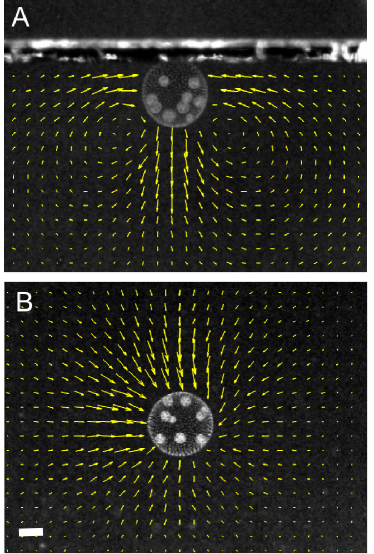
Figure 6: Volvox carteri swimming near a surface. Flow fields from particle imaging velocimetry of a colony swimming upward against a horizontal cover slip that is glued into the sample chamber (of size $2.5\times 2.5\times 5$ cm), as seen from the side (A), and the top (B). Images were taken at $\times 2$ magnification. Scale bar is $200$ $\mu$m.

In addition to allowing a controlled systematic disturbance to the behaviour of microorganisms in the form of light, this apparatus is also suitable to study the interactions of microorganisms with a surface, as the sample chambers can be made so large and so temperature-homogenized that the effect from other surfaces and thermal convection can be neglected. One interesting effect, discussed in more detail elsewhere waltzing , occurs when colonies swim upward to a horizontal surface and rotate in place. As the colonies are denser than the water in which they swim, and thus have a net external force acting on them, the far-field flow around them is described by a stokeslet pointing downwards. In the neighborhood of a no-slip surface, the stokeslet induces a set of image singularities which together produce a characteristic lobed flow field Blake . This is readily demonstrated by glueing a horizontal surface (a microscope coverslip) into the sample chamber and performing dual-view PIV. The results of this are shown in Fig. 6A,B, illustrating the fluid flow vector fields viewed from both the side and the top. From above, we see vectors oriented predominantly inward. This inward flow leads to complex behavior of nearby colonies waltzing .

When viewed from above as in Fig. 6B this setup also provides a means to monitor the rotational dynamics of colonies in great detail, providing accurate measurements of the mean rotational frequency, the noise in rotational motion, and lateral drifts. As mentioned earlier, the bottom-heaviness of the colonies keeps the colonial axis oriented vertically, allowing the daughters to serve as convenient markers to track rotation. Precise determination of time series of rotation can then be achieved by determining the correlation between successive images and a reference image, adjusted for centroid drift. The centroid dynamics itself serves as a sensitive measure of colony asymmetries, such as mismatch between the colonial axis and the axis defined by the center of buoyancy and the geometric center. Figure 7 shows the two components of the centroid position for a colony rotating against an upper surface, showing a clear periodic wobble at a frequency of $\sim 0.5$ Hz. The systematic drifts in position, which may be due to the swimming dynamics themselves or residual convective currents, are in any event below $2$ $\mu$m/s.

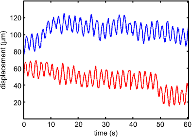
Figure 7: Tracking of spinning V. carteri. Shown are the $x$ (red) and $y$ (blue ) coordinates of a colony spinning near an upper surface with its axis vertical. Recorded at $10$ fps in convection controlled chamber. The oscillations represent a small periodic wobble in the colony centroid.

VI Conclusions

We presented an apparatus that can track swimming microorganisms in the size range $10-1000$ $\mu$m in 3D, without the influence of systematic bias due to beavioral stimuli, hydrodynamic interactions with surfaces, and convective background flows. As the apparatus can eliminate these biases, it can also be used to study the influence of each of them. The simplicity of the apparatus compared to other 3D tracking systems, and the software that is part of the supporting online material, make this system easily reproducible.

The heart of the apparatus can also be used as the basis for studies of more complex phenomena. For instance, the entire device can be mounted on a tiltable platform in order to examine the effects of varying direction of gravity with respect to the phototactic axis. Likewise, a rotatable chamber can be substituted for the ones discussed here in order to examine the effects of fluid vorticity on phototactic swimming Thorn .

VII Acknowledgments

We are grateful to D. Page-Croft, J. Milton, and T. Parkin for vital technical assistance, and to J.P. Gollub, J.T. Locsei, M. Polin and I. Tuval for important discussions. This work was supported by the EPSRC, Engineering and Biological Sciences program of the BBSRC, the Schlumberger Chair Fund, and DOE grant No. DE-AC02-06CH11357.

References

- (1) K. Hausmann, N. Hülsmann, and R. Radek, Protistology (Scheizerbart’sche Verlagsbuchhandlung, Stuttgart, 2003).
- (2) L.E. Graham and L.W. Wilcox, Algae (Prentice Hall, Upper Saddle River, NJ, 1999).
- (3) C.A. Solari, S. Ganguly, J.O. Kessler, R.E. Michod, and R.E. Goldstein, Proc. Natl. Acad. Sci. (USA) 103, 1353 (2006).
- (4) M.B. Short, C.A. Solari, S. Ganguly, T.R. Powers, J.O. Kessler, and R.E. Goldstein, Proc. Natl. Acad. Sci. (USA) 103, 8315 (2006).
- (5) T. Ishikawa and M. Hota, J. Exp. Biol. 22, 4452 (2006).
- (6) N.A. Hill and R.V. Vincent, J. Theor. Biol. 163, 223 (1993).
- (7) K. Schaller, R. David, and R. Uhl, Biophys. J. 73, 1562 (1997).
- (8) K. Drescher, K. Leptos, I. Tuval, T. Ishikawa, T.J. Pedley, and R.E. Goldstein, preprint (2009).
- (9) V.A. Vladimirov, P.V. Denissenko, T.J. Pedley, M. Wu, and I.S. Moskalev, Mar. Freshwater Res. 51, 589 (2000).
- (10) V.A. Vladimirov, M.S.C. Wu, T.J. Pedley, P.V. Denissenko, and S.G. Zakhidova, J. Exp. Biol. 207, 1203 (2004).
- (11) A.J. Goldman, R.G. Cox, and H. Brenner, Chem. Eng. Sci. 22, 637 (1967)
- (12) T.M. Squires, J. Fluid Mech. 443, 403 (2001).
- (13) H.C. Berg, Rev. Sci. Instrum. 42, 868 (1971).
- (14) G.J. Stephens, B. Johnson-Kerner, W. Bialek, and W.S. Ryu, PLOS Comput. Biol. 4, e1000028 (2008).
- (15) M. Wu, J.W. Roberts, and M. Buckley, Exp. Fluids 38, 461 (2005).
- (16) C.E. Willert and M. Gharib, Exp. Fluids 12, 353 (1992).
- (17) H. Pin Kao, and A.S. Verkman, Biophys. J. 67, 1291 (1994).
- (18) I.M. Peters, B.G. de Grooth, J.M. Schins, C.G. Figdor, and J. Greve, Rev. Sci. Instrum. 69, 2762 (1998).
- (19) L.P. Ghislain, N.A. Switz, and W.W. Webb, Rev. Sci. Instrum. 65, 2762 (1994).
- (20) H. Matsushita, T. Mochizuki, and N. Kaji, Rev. Sci. Instrum. 75, 541 (2004).
- (21) T.J. McGregor, D.J. Spence, and D.W. Coutts, Rev. Sci. Instrum. 79, 013710 (2008).
- (22) A.D. Dinsmore, E.R. Weeks, V. Prasad, A.C. Levitt, and D.A. Weitz, Appl. Opt. 40, 4152 (2001).
- (23) G. Rabut, and J. Ellenberg, J. Microsc. 216, 131 (2004).
- (24) H.G. Maas, A. Gruen, and D. Papantoniou, Exp. Fluids 15, 133 (1993).
- (25) K. Hoyer, M. Holzner, B. Lüthi, M. Guala, A. Liberzon, and W. Kinzelbach, Exp. Fluids 39, 923 (2005).
- (26) A.M. Grillet, C.F. Brooks, C.J. Bourdon, and A.D. Gorby, Rev. Sci. Instrum. 78, 093902 (2007).
- (27) J.R. Strickler, Philos. Trans. Roy. Soc. London B, Biol. Sci. 353, 671 (1998).
- (28) R. Thar, N. Blackburn, and M. Kühl, Appl. Environ. Microbiol. 66, 2238 (2000).
- (29) H. Sakaguchi and K. Iwasa, Plant Cell Physiol. 20, 909 (1979).
- (30) M.C. Cross and P.C. Hohenberg, Rev. Mod. Phys. 65, 851 (1993).
- (31) P.N. Segre, E. Herbolzheimer, and P. M. Chaikin, Phys. Rev. Lett. 79, 2574 (1997).
- (32) S.-Y. Tee, P.J. Mucha, L. Cipelletti, S. Manley, M.P. Brenner, P.N. Segre, and D.A. Weitz, Phys. Rev. Lett. 89, 054501 (2002).
- (33) D.R. Mitchell, J. Phycol. 36, 261 (2000).
- (34) D.B. Weibel, P. Garstecki, D. Ryan, W.R. DiLuzio, M. Mayer, J.E. Seto, and G.M. Whitesides, Proc. Natl. Acad. Sci. (USA) 102, 11963 (2005).
- (35) See: http://www.physics.emory.edu/weeks/idl/.
- (36) H. Xu, Meas. Sci. Technol. 19, 075105 (2008)
- (37) J. Gelles, B.J. Schnapp, and M.P. Sheetz, Nature 331, 450 (1988).
- (38) M.K. Cheezum, W.F. Walker, and W.H. Guilford, Biophys. J. 81, 2378 (2001).
- (39) R.N. Kieft, K.R.A.M. Schreel, G.A.J. van der Plas, and C.C.M. Rindt, Exp. Fluids 33, 603 (2002).
- (40) H.C. Berg and D.A. Brown, Nature 239, 500 (1972).
- (41) D.L. Kirk and M.M. Kirk, Dev. Biol. 96, 493 (1983).
- (42) C.A. Solari, R.E. Michod, and R.E.Goldstein, J. Phycol. 44, 1395 (2008).
- (43) J.R. Blake, Proc. Camb. Phil. Soc. 70, 303 (1971).
- (44) G.J. Thorn, K. Drescher, R.N. Bearon, and R.E. Goldstein, preprint (2008).