Dwell-time distributions in quantum mechanics

Abstract

Some fundamental and formal aspects of the quantum dwell time are reviewed, examples for free motion and scattering off a potential barrier are provided, as well as extensions of the concept. We also examine the connection between the dwell time of a quantum particle in a region of space and flux-flux correlations at the boundaries, as well as operational approaches and approximations to measure the flux-flux correlation function and thus the second moment of the dwell time, which is shown to be characteristically quantum, and larger than the corresponding classical moment even for freely moving particles.

I Introduction

Time observables in quantum mechanics have a long and debated history Muga-book . In spite of the fact that random time variables, measured after a system is prepared, are common in laboratories, most often it has been argued that questions about time in quantum mechanics should best be left alone, as illustrated by the frequent reference to Pauli’s theorem. Alternatively, the emphasis has been laid on characteristic times, i.e. single time quantities characterizing a process such as tunneling, or decay. This, in many ways, runs counter to the usual procedure in quantum mechanics, where additionally to the average value of a quantity we require prediction of higher order moments of that quantity; in other words, the probability distribution.

With regard to the time-of-arrival observable several such distributions have been proposed and studied, see volume 1 of “Time in Quantum Mechanics” toabook , or MuLea-PR-2000 . In this chapter we analyze the dwell time, which appears to be a much simpler time observable because the associated operator will indeed be self-adjoint (over the adequate domain). At first sight, it could be thought that this statement contradicts Pauli’s theorem, which asserts that no self-adjoint time observable can exist with canonical commutation relations with a semi bound Hamiltonian. However, the dwell time is an interval quantity, as opposed to the instant quantity that the time of arrival describes. Its associated operator, therefore, should commute with the Hamiltonian, as opposed to presenting canonical commutation with it.

The dwell time of a particle in a region of space and its close relative, the delay time Smith60 , are rather fundamental quantities that characterize the duration of collision processes, the lifetime of unstable systems EkSie-AP-1971 , the response to perturbations JaWa-PRA-1989 , ac-conductance in mesoscopic conductors Bu , or the properties of chaotic scattering MW . In addition, the importance of dwell and delay times is underlined by their relation to the density of states, and to the virial expansion in statistical mechanics Nuss2002 . We could thus hardly fail to study and characterize in detail such a prominent quantity. For a sample of theoretical studies on the quantum dwell time see EkSie-AP-1971 ; JaWa-PRA-1989 ; SK91 ; BSM94 ; LM94 ; Nuss2002 ; S02 ; DEMN04 ; Y04 ; S04 ; LV04 ; W06 ; K07 ; S07 ; BS08 ; charac ; chokoloki . A recurrent topic has been its role and decomposition in tunneling collisions. Instead, we shall focus here on a different, so far overlooked but fundamental aspect, namely, the measurability and physical implications of its distribution, and its second moment.

Despite the nice properties of the dwell-time operator, the relevance of the concept and average value in many different fields, or the apparent formal simplicity stated above, the dwell time is actually rather subtle and remains elusive and challenging in many ways. In particular, a direct and sufficiently non-invasive measurement, so that the statistical moments are produced by averaging over individual dwell-time values, is yet to be discovered. If the particle is detected (and thus localized) at the entrance of the region of interest, its wavefunction is severely modified (“collapsed”), so that the times elapsed until a further detection when it leaves the region do not reproduce the ideal dwell-time operator distribution, and depend on the details of the localization method. Proposals for operational, i.e., measurement-based approaches to traversal times based on model detectors which study the effect of localization have been discussed by Palao et al. PaMuBrJa-PLA-1997 and by Ruschhaupt Ru-PLA-1998 . For attempts to measure the dwell time with continuous or kicked “clocks” coupled to the particle’s presence in the region see chokoloki ; ASM93 . All operational approaches to the quantum dwell time known so far have provided only its average, and indirectly, by deducing it from its theoretical relation to some other observable with measurable average. The average is obtained for example by a “Larmor clock”, using a weak homogeneous magnetic field in the region $D$ and the amount of spin rotations of an incident spin-$\frac{1}{2}$ particle Baz-SJNP-1967 ; Ry-SJNP-1967 ; Bue-PRB-1983 . An optical analogue is provided by the “Rabi clock” Bra-JPB-1997 . It can also be deduced from average passage times at the region boundaries charac , as well as by measuring the total absorption if a weak complex absorbing potential acts in the region CP1 ; CP2 ; CP3 . This last setup could be implemented with cold atoms and lasers as described in DEMN04 ; CP4 and will be discussed in Sect. IV.2.

The chapter is organized as follows: the first sections are devoted to fundamental and formal aspects (Sect. 2), examples (Sects. 3 and 4), or extensions (Sect. 5) of the dwell-time concept and operator, whereas Sect. 6 tackles the relationship between the moments of the dwell-time operator and flux-flux correlation functions (ffcf) Munoz , generalizing an approach by Pollak and Miller PoMi-PRL-1984 . They showed that the average stationary dwell time agrees with the first moment of a microcanonical ffcf. We shall see that this relation holds also for the second moment, but not for higher moments, and extend their analysis to the time-dependent (wavepacket) case. We shall also discuss a possible scheme to measure ffcf’s, thus paving the way towards experimental access to quantum features of the dwell-time distribution.

II The Dwell Time Operator

Unlike other time quantities, there has been a broad consensus on the operator representation of the dwell time EkSie-AP-1971 ; JaWa-PRA-1989 . For one particle evolving unitarily with Hamiltonian $\widehat{H}$ in region $D$, which we limit here to one dimension for simplicity, $D=\{x:x_{1}\leq x\leq x_{2}\}$, it takes the form

$$\widehat{T}_{D} = \int_{-\infty}^{\infty}\mathrm{d}t\,\widehat{\chi}_{D}(t)=\int_{-\infty}^{\infty}\mathrm{d}t\,\mathrm{e}^{\mathrm{i}\widehat{H}t/\hbar}\chi_{D}(\widehat{x})\,\mathrm{e}^{-\mathrm{i}\widehat{H}t/\hbar}\;,$$ (1)

where $\widehat{\chi}_{D}(t)$ is the (Heisenberg) projector onto $D$, and $\chi_{D}(\widehat{x})=\widehat{\chi}_{D}(0)=\int_{x_{1}}^{x_{2}}dx|x\rangle\langle x|$. Without delving too far in the functional analysis definition, i.e. into the proper description of its domain and of its adjoint, we can see that $\widehat{T}_{D}$ will be self-adjoint (we shall come back to this issue after studying the specific example of the free particle Hamiltonian in Sect. III). At any rate, it is clear that, at least formally, this operator commutes with the Hamiltonian, as can be seen from what follows:

$$\widehat{T}_{D}\mathrm{e}^{-\mathrm{i}\widehat{H}t/\hbar} = \int_{-\infty}^{\infty}\mathrm{d}\tau\,\mathrm{e}^{\mathrm{i}\widehat{H}\tau/\hbar}\chi_{D}(\widehat{x})\,\mathrm{e}^{-\mathrm{i}\widehat{H}(\tau+t)/\hbar}$$

$$= \int_{-\infty}^{\infty}\mathrm{d}\tau\,\mathrm{e}^{\mathrm{i}\widehat{H(}\tau-t)/\hbar}\chi_{D}(\widehat{x})\,\mathrm{e}^{-\mathrm{i}\widehat{H}\tau/\hbar}=\mathrm{e}^{-\mathrm{i}\widehat{H}t/\hbar}\widehat{T}_{D}\,\,.$$

The commutation of $\widehat{T}_{D}$ and the Hamiltonian leads us to search for the eigenfunctions of dwell time in the stationary eigenspaces of the latter. Let $\alpha$ be the degeneracy index for these eigenspaces, such that $\widehat{H}|E,\alpha\rangle=E|E,\alpha\rangle$. We easily obtain the matrix elements of $\widehat{T}_{D}$ in the corresponding eigenspace,

$$\widehat{T}_{D}|E,\alpha\rangle=2\pi\hbar\sum_{\beta}\langle E,\beta|\chi_{D}(\widehat{x})|E,\alpha\rangle\,|E,\beta\rangle\;.$$ (3)

We may thus reduce the problem of eigenvalues and eigenfunctions of the dwell-time operator to a set of matrix diagonalization problems in each of the eigenspaces of the Hamiltonian.

Except in Sect. V we shall assume that the Hamiltonian holds a purely continuous spectrum with degenerate (delta-normalized) scattering eigenfunctions $|\phi_{\pm k}\rangle$ corresponding to incident plane waves $|\pm k\rangle$, with energy $E=k^{2}\hbar^{2}/(2m)$, normalized as $\langle k|k^{\prime}\rangle=\langle\phi_{k}|\phi_{k^{\prime}}\rangle=\delta(k-k^{\prime})$.

Following the same manipulation done for the $S$-operator in one-dimensional scattering theory charac , it is convenient to define an on-the-energy-shell $2\times 2$ dwell-time matrix $\mathsf{T}$, by factoring out an energy delta,

$$\langle\phi_{k}|\widehat{T}_{D}|\phi_{k}^{\prime}\rangle=\delta(E-E^{\prime})\frac{|k|\hbar^{2}}{m}\mathsf{T}_{kk^{\prime}}\;,$$ (4)

where $E^{\prime}=k^{\prime 2}\hbar^{2}/(2m)$ and

$$\mathsf{T}_{kk^{\prime}}=\langle\phi_{k}|{\chi}_{D}(\widehat{x})|\phi_{k^{\prime}}\rangle\frac{2\pi m}{|k|\hbar},\;\;E=E^{\prime}\;.$$ (5)

In particular, $\mathsf{T}_{kk}$ is the average dwell time for a finite space region defined by Büttiker in the stationary regime Bue-PRB-1983 ,

$$\mathsf{T}_{kk}=\frac{1}{|j(k)|}\int_{x_{1}}^{x_{2}}\mathrm{d}x\,|\phi_{k}(x)|^{2}\;,$$ (6)

where $j(k)$ is the incoming flux associated with $|\phi_{k}\rangle$.

An intriguing peculiarity of the quantum dwell time is that the diagonalization of $\mathsf{T}$ at a given energy provides in general two distinct eigenvalues $t_{\pm}(k)$, $k>0$, and corresponding eigenvectors $|t_{\pm}(k)\rangle$, even in cases in which only a single classical time exists, such as free motion, or transmission above the barrier; some explicit examples are discussed below. A consequence is a broader variance of the quantum dwell-time distribution compared to the classical one.

The quantum dwell-time distribution for a state $|\psi\rangle=|\psi(t=0)\rangle$, is formally given by

$$\Pi_{\psi}(\tau)=\langle\psi|\delta(\widehat{T}_{D}-\tau)|\psi\rangle\;,$$ (7)

since the self-adjointness of the dwell-time operator implies that the spectral theorem applies, and that operator moments coincide with the moments of the distribution. We shall not consider in this work other sources of fluctuations such as mixed states or ensembles of Hamiltonians. In these two cases one could compute distributions of average dwell times, whereas here we shall be interested in the distribution of the dwell time itself, but only for pure states and a single Hamiltonian.

On computing the distribution of dwell times we run into the difficulty, mentioned above, that the dwell-time operator is multiply degenerate, and that it is not altogether easy to de-scramble the relation between a given $t$ and the corresponding set of momenta. It is useful in this case to profit from the spectral theorem to compute the generating function of the dwell-time distribution, defined as

$$f_{\psi}(\omega)=\int_{0}^{\infty}\mathrm{d}t\,\mathrm{e}^{\mathrm{i}\omega t}\,\Pi_{\psi}(t)=\langle\psi|\mathrm{e}^{\mathrm{i}\omega\widehat{T}_{D}}|\psi\rangle\;.$$ (8)

Normalizing the dwell-time eigenvectors so as to have the resolution of the identity

$$\widehat{1}=\sum_{\alpha}\int_{0}^{\infty}\mathrm{d}k|t_{\alpha}(k)\rangle\langle t_{\alpha}(k)|\;,$$ (9)

$f_{\psi}$ can be written as

$$f_{\psi}(\omega)=\int_{0}^{\infty}\mathrm{d}k\,\Big{[}\mathrm{e}^{\mathrm{i}\omega t_{+}(k)}\langle\psi|t_{+}(k)\rangle\langle t_{+}(k)|\psi\rangle+\mathrm{e}^{\mathrm{i}\omega t_{-}(k)}\langle\psi|t_{-}(k)\rangle\langle t_{-}(k)|\psi\rangle\Big{]}\;,$$ (10)

and, hence,

$$\Pi_{\psi}(t) = \int_{-\infty}^{\infty}\frac{d\omega}{2\pi}\,\mathrm{e}^{-\mathrm{i}\omega t}f_{\psi}(\omega)$$ (11)

$$= \int_{0}^{\infty}\mathrm{d}k\left[\delta(t-t_{+})|\langle\psi|t_{+}\rangle|^{2}+\delta(t-t_{-})|\langle\psi|t_{-}\rangle|^{2}\right]\;.$$

The average of the dwell time for a wavepacket can be given in terms of the position probability density in correspondence (unlike its second moment, as shown below) to the expression for an ensemble of classical particles. It reads JaWa-PRA-1988 ; MuBrSa-PLA-1992

$$\langle\psi|\widehat{T}_{D}|\psi\rangle=\int_{-\infty}^{\infty}\mathrm{d}t\int_{x_{1}}^{x_{2}}\mathrm{d}x\,|\psi(x,t)|^{2}=\int_{0}^{\infty}\mathrm{d}k\,|\langle k|{\psi}^{in}\rangle|^{2}\mathsf{T}_{kk}\;,$$ (12)

where $\psi(x,t)=\int_{0}^{\infty}\mathrm{d}k\,\langle\phi_{k}|\psi\rangle\exp(-\mathrm{i}\hbar k^{2}t/2m)\phi_{k}(x)$ is the time-dependent wave packet and we assume, here and in the rest of the Chapter, incident wavepackets with positive momentum components. To write Eq. (12) use has been made of the standard scattering relation $\langle\phi_{k}|\psi\rangle=\langle k|\psi^{in}\rangle$, where $\langle x|k\rangle=(2\pi)^{-{1/2}}\exp(\mathrm{i}kx)$, and $\psi^{in}$ is the freely-moving asymptotic incoming state of $\psi$. Space-time integrals of the form (12) had been used to define time delays by comparing the free motion to that with a scattering center and taking the limit of infinite volume GoWa-book .

The second moment takes the form, as before for wavepackets with incident positive momentum components,

$$\left\langle\widehat{T}_{D}^{2}\right\rangle = \int_{0}^{\infty}\mathrm{d}k(\mathsf{T}^{\,2})_{kk}|\langle k|\psi^{in}\rangle|^{2}=\int_{0}^{\infty}\mathrm{d}k(|\mathsf{T}_{kk}|^{2}+|\mathsf{T}_{k-k}|^{2})|\langle k|\psi^{in}\rangle|^{2}$$ (13)

$$= \int_{0}^{\infty}\mathrm{d}k\frac{4\pi^{2}m^{2}}{\hbar^{2}k^{2}}\Bigg{[}\Big{(}\int_{x_{1}}^{x_{2}}\mathrm{d}x\,|\phi_{k}(x)|^{2}\Big{)}^{2}+\Big{|}\int_{x_{1}}^{x_{2}}\!\mathrm{d}x\,\phi_{k}^{*}(x)\phi_{-k}(x)\Big{|}^{2}\Bigg{]}|\langle k|\psi^{in}\rangle|^{2}\;,$$

with a term without classical counterpart.

III The Free Particle Case

In order to get a better grasp of the abstract results, it is adequate to illustrate them with the explicitly solvable free-particle case for a region $D$ that extends from $x_{1}=0$ to $x_{2}=L$. Indeed the humble freely moving particle turns out to be rather interesting and surprisingly complex with regard to the dwell time. The free-particle Hamiltonian is doubly degenerate; we can choose the degeneracy indices to coincide with the sign of the momentum, and, on computation, with due attention to the different normalization of the energy and the momentum eigenfunctions, we find the following generalized eigenfunctions of the free dwell-time operator:

$$|t_{\pm}(k),D\rangle=\frac{1}{\sqrt{2}}\left[|k\rangle\pm\mathrm{e}^{\mathrm{i}kL}|-k\rangle\right]\;,$$ (14)

where

$$t_{\pm}(k)=\frac{mL}{k\hbar}\left(1\pm\frac{1}{kL}\sin{kL}\right)$$ (15)

are the corresponding eigenvalues, in clear contrast to the classical time $t_{\mathrm{class}}=mL/(|k|\hbar)$, see Fig 1.

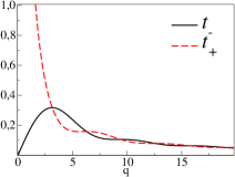
Figure 1: Eigenvalues of the dwell-time-operator as a function of $q=kL$, in units $mL^{2}/\hbar$, for a freely moving particle in a region of length $L$

It is important to notice that the inverse function is multivalued. Due to this multivaluedness we have kept generalized eigenfunctions with the dimensionality of $|k\rangle$, instead of normalizing them to the delta function in dwell times. With this normalization it is easy to check that the resolution of the identity has the form (9).

Interestingly, $t_{-}(k)$ tends to zero as $k\to 0$, one more very non-classical effect that is better understood from the coordinate representation of the eigenvectors,

$$\langle x|t_{+}\rangle = \frac{\mathrm{e}^{\mathrm{i}kL/2}}{\pi^{1/2}}\cos[k(x-L/2)]\;,$$

$$\langle x|t_{-}\rangle = \frac{\mathrm{i}\mathrm{e}^{\mathrm{i}kL/2}}{\pi^{1/2}}\sin[k(x-L/2)]\;,$$ (16)

symmetric and antisymmetric with respect to the interval center. $\langle x|t_{-}\rangle$ vanishes at $L/2$, so the particle density tends to vanish in $D$ with longer wavelengths as $k\to 0$.

The dwell-time operator for an interval $D^{\prime}=[a,a+L]$ is obtained from the one above by translation,

$$\widehat{T}_{D\,^{\prime}}=\mathrm{e}^{-\mathrm{i}a\widehat{k}}\widehat{T}_{D}\mathrm{e}^{\mathrm{i}a\widehat{k}}\;,$$ (17)

and, as a consequence, the eigenvalues are not modified, while the new eigenfunctions are easily computed as

$$|t_{\pm}(k),D^{\prime}\rangle = \mathrm{e}^{-\mathrm{i}a\widehat{k}}|t_{\pm}(k),D\rangle$$ (18)

$$= \frac{1}{\sqrt{2}}\left[\mathrm{e}^{-\mathrm{i}ak}|k\rangle\pm\mathrm{e}^{\mathrm{i}k(a+L)}|-k\rangle\right]\;.$$

It is straightforward to compute directly the action of $\widehat{T}_{D}$ in the wavenumber representation,

$$\langle k|\widehat{T}_{D}|\psi\rangle=\frac{mL}{|k|\hbar}\left[\widetilde{\psi}(k)+\mathrm{e}^{-\mathrm{i}kL}\frac{1}{kL}\sin\left({kL}\right)\widetilde{\psi}(-k)\right]\;,$$ (19)

where $\widetilde{\psi}(k)=\langle k|\psi\rangle$. This allows us to study the functional aspects of the operator. In particular, it is easy to check, using the requirement of normalizability, that the domain of the operator is given by functions such that $\widetilde{\psi}(k)/k\rightarrow 0$ as $k\rightarrow 0$. The requirement of symmetry does not add further limitations to the domain. As to the deficiency indices, they are computed to be $(0,0)$. These computations are carried out for the interval $D=[0,L]$, but, given the unitary equivalence of other intervals of the same length, see Eq. (17), the same results carry over for regions composed of an arbitrary number of closed intervals.

It should come as no surprise that functions in the domain of the (free particle) dwell-time operator must vanish at $p=0$ fast enough, since the characteristic evolution of a generic wavefunction is dictated by the free propagator, with its $t^{-1/2}$ temporal behavior. This entails the divergence of the dwell time unless the state has no $p=0$ component and the amplitude decay is faster (for a simple analysis, see DEM02 ). The divergence of the average dwell time for states with nonvanishing $p=0$ components also occurs for ensembles of classical particles.

To calculate the distribution $\Pi_{\psi}(t)$, see Eqs. (10) and (11), we have in this case the characteristic function

$$f_{\psi}(\omega) = \int_{-\infty}^{\infty}\mathrm{d}k\,\mathrm{e}^{\mathrm{i}\omega mL/(|k|\hbar)}\cos\left[\frac{\omega m}{k^{2}\hbar}\sin(kL)\right]\,|\widetilde{\psi}(k)|^{2}+$$ (20)

$$\,\mathrm{i}\,\int_{-\infty}^{\infty}\mathrm{d}k\,\mathrm{e}^{\mathrm{i}\omega mL/(|k|\hbar)}\sin\left[\frac{\omega m}{|k|k\hbar}\sin(kL)\right]\quad\mathrm{e}^{-\mathrm{i}kL}\widetilde{\psi}(k)\overline{\widetilde{\psi}(-k)}\;.$$

The distribution $\Pi_{\psi}(t)$ has support only on the positive semi-axis, as can be seen from the explicit expression for the eigenvalues. This, in turn, is a nontrivial check of the correctness of the definition.

A further initially surprising result of this analysis is that for highly monochromatic wavepackets (i.e., highly concentrated in one point in the momentum representation), the probability density for dwell times is generically bimodal because of the two eigenvalues $t_{\pm}(k)$ expounded in Eq. (15). An experimental verification of the eigenvalues, and of the quantum nature of the dwell time, could be realized with the aid of a matter-wave mirror located at a point $X>L$, reflecting an incident plane wave $|k\rangle$. The resulting standing wave would take the form, up to a global phase factor,

$$|\psi_{X}\rangle=|k\rangle-\mathrm{e}^{-2\mathrm{i}kX}|-k\rangle\;.$$ (21)

We may now compute the average dwell time between $0$ and $L$,

$$\langle\psi_{X}|\mathsf{T}|\psi_{X}\rangle = \mathsf{T}_{kk}+\mathsf{T}_{-k-k}-2\mathrm{Re}(\mathrm{e}^{-2\mathrm{i}kX}T_{k-k})$$ (22)

$$= 2\frac{Lm}{|k|\hbar}\left\{1-\cos[k(L+2X)]\frac{\sin(kL)}{kL}\right\}\;,$$

which oscillates between the maximum and minimum values $2t_{\pm}$, see (15); they occur at specific locations of the mirror, namely,

$$X_{-} = -\frac{L}{2}+\frac{\pi n}{k}\;,$$ (23)

$$X_{+} = -\frac{L}{2}+\frac{\pi n}{k}+\frac{\pi}{2k}\;,$$ (24)

($n$ integer such that $X>L$), for which the standing wave $|\psi_{X}\rangle$ becomes proportional to $|t_{\pm}\rangle$. The proportionality factor $2^{1/2}$ accounts for the fact that the extrema correspond to twice the eigenvalues, which is easy to interpret physically with reference to a corresponding classical scenario: the classical particle under similar circumstances would traverse the region twice, first rightwards and then leftwards. For any $X$ between the priviledged values $X_{\pm}$ given above, $|\psi_{X}\rangle$ is a linear superposition of the dwell time eigenvectors and thus the resulting average dwell time lies in a continuum between two times the eigenvalues. In a proposed experiment a highly monochromatic continuous beam would be sent towards the mirror and the particle density could be measured between $0$ and $L$ by fluorescence or other means. The oscillations of the signal as a function of $X$ would be in sharp contrast to the classical case, for which the the beam density and dwell time would remain unaffected by a change of the mirror’s position.

III.1 A comparison with classicality

We have already noticed some of the peculiarities of the quantum dwell time compared to the classical dwell time. Here we elaborate this comparison further. Consider a classical ensemble of free particles, described by the initial probability density on phase space, $F(x,p)$. The dwell-time distribution for this case is given by

$$\Pi_{\mathrm{class}}(t) = \int dx\,dp\,\delta\left(t-\frac{mL}{|p|}\right)\,F(x,p)$$ (25)

$$= \frac{mL}{t^{2}}\int dx\,\left[F\left(x,\frac{mL}{t}\right)+F\left(x,\frac{mL}{-t}\right)\right]\;,$$

that is to say, the marginal momentum distribution evaluated at $mL/t$ and $-mL/t$, and multiplied by the normalization factor $mL/t^{2}$. On the other hand, the distribution (11) obtained from Eq. (20) includes effects of interferences between positive and negative momentum components, in two different ways. In the first place, there is the obvious interference of the last line of (20); but, additional to this, the argument of the cosine also reveals these effects. In order to see better this point, let us examine a different operator,

$$\widehat{t}_{D}:=\widehat{\lambda}_{+}\widehat{T}_{D}\widehat{\lambda}_{+}+\widehat{\lambda}_{-}\widehat{T}_{D}\widehat{\lambda}_{-}=mL/|\widehat{p}|\;,$$ (26)

where $\widehat{\lambda}_{\pm}$ are the projectors onto the positive/negative momentum subspaces. Notice that $\widehat{\lambda}_{\pm}$ do not commute with $\widehat{T}_{D}$. The last form in Eq. (26), specific of free motion, is particularly transparent and reproduces the one of the classical dwell time. The eigenfunctions are $|\pm k\rangle$, $k>0$, and the corresponding eigenvalues are twofold degenerate and equal to the classical time, $mL/\hbar|k|$. The distribution of dwell times for this operator, and for positive-momentum states, is given by

$$\pi_{\psi}(\tau)=\frac{mL}{\hbar\tau^{2}}\left|\widetilde{\psi}\left(\frac{mL}{\hbar\tau}\right)\right|^{2}\;,$$ (27)

which coincides with the classical distribution for initial wave functions whose support is limited to positive momenta. In this manner we see that the distribution (11) incorporates interferences even if only positive momenta are present. To be even more explicit, observe that, for a state $\psi$ with only positive momenta components, the second moment of the dwell-time operator (1) is given by

$$\left\langle\widehat{T}_{D}^{2}\right\rangle = \int_{0}^{\infty}\mathrm{d}k(\mathsf{T}^{\,2})_{kk}|\widetilde{\psi}(k)|^{2}=\int_{0}^{\infty}\mathrm{d}k(|\mathsf{T}_{kk}|^{2}+|\mathsf{T}_{k-k}|^{2})|\widetilde{\psi}(k)|^{2}$$ (28)

$$= \int_{0}^{\infty}\mathrm{d}k\,\frac{m^{2}L^{2}}{k^{2}\hbar^{2}}\,\left[1+\frac{1}{k^{2}L^{2}}\sin^{2}\left({kL}\right)\right]\left|\widetilde{\psi}(k)\right|^{2}\;,$$

which contrasts with

$$\left\langle\widehat{{t}}^{\,\,2}_{D}\right\rangle=\int_{0}^{\infty}\mathrm{d}k\,\frac{m^{2}L^{2}}{k^{2}\hbar^{2}}\,\left|\widetilde{\psi}(k)\right|^{2}\,,$$

thus indicating that indeed the second term is due to quantum interference.

As indicated above, there is another rather striking way of seeing this point, by considering a highly monochromatic wavepacket. The classical distribution would have a very sharply defined peak around $mL/p_{0}$, where $p_{0}$ is the central momentum of the wavefunction, $p_{0}=k_{0}\hbar$; on the other hand, the quantum distribution would have two sharp peaks, centered on $t_{+}(k_{0})$ and $t_{-}(k_{0})$ respectively. The distance between peaks goes to zero as $p_{0}$ increases, as was to be expected since that is the classical limit.

The on-the-energy-shell version of $\widehat{t}_{D}$, $\mathsf{t}$, is also worth examining. By factoring out an energy delta function as in Eq. (4) we get for a plane wave $|k\rangle$ the average $\mathsf{t}_{kk}=mL/(\hbar k)$, which is equal to $\mathsf{T}_{kk}$, but the second moment differs, $(\mathsf{t}^{2})_{kk}=(\mathsf{t}_{kk})^{2}=(\mathsf{T}_{kk})^{2}\leq(\mathsf{T}^{2})_{kk}$, see Fig. 1; in other words, the variance on the energy shell is zero since only one eigenvalue is possible for $\mathsf{t}$. Contrast this with the extra term in Eq. (28), which again emphasizes the non-classicality of the dwell-time operator $\widehat{T}_{D}$ and its quantum fluctuation.

IV The scattering case

Let us now study the dwell time in a potential barrier or well without bound states, that is, the dwell time in an interval which coincides with the finite support of the potential $V(x)$, which presents no bound states. For simplicity, we shall assume as before that this interval starts at point $x=0$ and has length $L$. We shall use the complete basis of incoming scattering stationary states, $\left|k^{+}\right\rangle$, with the following position representation, for $k>0$,

$$\left\langle x\big{|}k^{+}\right\rangle=\frac{1}{\sqrt{2\pi}}\left\{\begin{array}[]{ll}\mathrm{e}^{\mathrm{i}kx}+R^{l}(k)\mathrm{e}^{-\mathrm{i}kx}&\textrm{for }x<0\\ T^{l}(k)\mathrm{e}^{\mathrm{i}kx}&\textrm{for }x>L\end{array}\right.\;,$$ (29)

whereas, for $k<0$, we have

$$\left\langle x\big{|}k^{+}\right\rangle=\frac{1}{\sqrt{2\pi}}\left\{\begin{array}[]{ll}T^{r}(-k)\mathrm{e}^{\mathrm{i}kx}&\textrm{for }x<0\\ \mathrm{e}^{\mathrm{i}kx}+R^{r}(-k)\mathrm{e}^{-\mathrm{i}kx}&\textrm{for }x>L\end{array}\right.$$ (30)

(the superscripts $l,r$ in $T^{l}$, $R^{l}$, and $T^{r}$, $R^{r}$ stand for left and right incidence). We have omitted any explicit expression in the interval $[0,L]$ because of the potential dependence. The eigenvalues and eigenstates of the dwell-time operator can be formally computed using $\widehat{H}\left|k^{+}\right\rangle=(k^{2}\hbar^{2}/2m)\left|k^{+}\right\rangle$. To that end define

$$\xi(k)=\frac{\left\langle k^{+}\left|\chi_{D}(\widehat{x})\right|k^{+}\right\rangle}{2\sigma(k)}\;,$$ (31)

where

$$\sigma(k)=\left|\left\langle-k^{+}\left|\chi_{D}(\widehat{x})\right|k^{+}\right\rangle\right|\;,$$ (32)

and

$$\mathrm{e}^{\mathrm{i}\varphi(k)}=\frac{\left\langle-k^{+}\left|\chi_{D}(\widehat{x})\right|k^{+}\right\rangle}{\sigma(k)}\;.$$ (33)

Additionally, for the sake of compactness in later formulae, let

$$\mu(k)=\frac{1}{2}\left[\xi(-k)-\xi(k)\right]\,.$$ (34)

We then have that the eigenvalues of the dwell-time operator are given by

$$t_{\pm}(k)=\frac{2\pi m\sigma(k)}{|k|\hbar}\,\left[\frac{\xi(k)+\xi(-k)}{2}\pm\sqrt{1+\mu^{2}(k)}\right]\;,$$ (35)

while the eigenfunctions are

$$|t_{\pm}(k)\rangle=N_{\pm}\left\{\left|k^{+}\right\rangle+\mathrm{e}^{\mathrm{i}\varphi(k)}\left[\mu(k)\pm\sqrt{1+\mu^{2}(k)}\right]\left|-k^{+}\right\rangle\right\}\;,$$ (36)

and the normalization is given by

$$N_{\pm}=\frac{1}{\sqrt{2}}\left[1+\mu^{2}\pm\mu\sqrt{1+\mu^{2}(k)}\right]^{-1/2}\;.$$ (37)

In fact, we can relate the quantities $\xi(k)$, $\sigma(k)$ and $\varphi(k)$ to scattering data whenever the support of the scattering potential is completely included in the region $D$. Let $\bar{\chi}_{D}(x)$ be the complementary function to $\chi_{D}(x)$. We can compute $\left\langle k^{\prime\,+}\right|\bar{\chi}(\widehat{x})\left|k^{+}\right\rangle$ explicitly, and, using unitarity and the conditions this imposes on the scattering amplitudes, we are led to the following expressions (where we omit the arguments of the scattering amplitudes, since all are evaluated at $k$, and denote derivative with respect to $k$ as $\partial_{k}$):

$$\left\langle k^{+}\left|\chi_{D}(\widehat{x})\right|k^{+}\right\rangle = \frac{L}{2\pi}\left|T^{l}\right|^{2}+\frac{\mathrm{i}}{2\pi}\left[R^{l}\partial_{k}\bar{R}^{l}+T^{l}\partial_{k}\bar{T}^{l}\right]+\frac{\mathrm{i}}{4\pi k}\left[\bar{R}^{l}-R^{l}\right]\,,$$

$$\left\langle-k^{+}\left|\chi_{D}(\widehat{x})\right|-k^{+}\right\rangle = \frac{L}{2\pi}\left[1+\left|R^{r}\right|^{2}\right]+\frac{\mathrm{i}}{2\pi}\left[R^{r}\partial_{k}\bar{R}^{r}+T^{r}\partial_{k}\bar{T}^{r}\right]$$

$$+ \frac{\mathrm{i}}{4\pi k}\left[\mathrm{e}^{-2\mathrm{i}kL}\bar{R}^{r}-\mathrm{e}^{2\mathrm{i}kL}R^{r}\right]\,,$$

$$\left\langle-k^{+}\left|\chi_{D}(\widehat{x})\right|k^{+}\right\rangle = \frac{L}{2\pi}T^{l}\bar{R}^{r}+\frac{\mathrm{i}}{2\pi}\left[R^{l}\partial_{k}\bar{T}^{r}+T^{l}\partial_{k}\bar{R}^{r}\right]+\frac{\mathrm{i}}{4\pi k}\left[\bar{T}^{r}-\mathrm{e}^{2\mathrm{i}kL}T^{l}\right]\,.$$

Notice that the second term of each of the previous expressions can be identified with the corresponding on-shell matrix elements of $-(\mathrm{i}m/k\hbar)S^{\dagger}\partial_{k}S$. That is, with Smith’s delay time!

IV.1 The Square Barrier

For the specific case of a square barrier, in which $V(x)=V_{0}[\theta(x-L)-\theta(x)]$, with $\theta(x)$ being Heaviside’s unit step function, we can put to good use the symmetries of the Hamiltonian, namely $x\to L-x$ and $k\to-k$. These are realized on the scattering states as

$$\langle L-x|k^{+}\rangle=\mathrm{e}^{\mathrm{i}kL}\langle x\left|-k^{+}\right\rangle\;,$$

whence $\xi(k)=\xi(-k)$, and $\mu(k)=0$. Furthermore,

$$\left\langle k^{+}\left|\chi_{D}(\widehat{x})\right|k^{+}\right\rangle=\frac{L\left|T(k)\right|^{2}}{2\pi\kappa^{2}}\left\{k^{2}-\frac{mV_{0}}{\hbar^{2}}\left[1+\frac{1}{2\kappa L}\sin\left({2\kappa L}\right)\right]\right\}\;,$$

where $\kappa=\sqrt{k^{2}-2mV_{0}/\hbar^{2}},$ real and positive for positive above-the-barrier momenta, and with positive imaginary part for tunneling momenta. After some cumbersome algebra, one readily obtains

$$t_{\pm}(k)=\frac{\left|T(k)\right|^{2}mL}{2\hbar\left|k\right|\kappa^{2}}\left[k^{2}+\kappa^{2}\pm\left(\kappa^{2}-k^{2}\right)\cos{\kappa L}\right]\left[1\pm\frac{1}{kL}\sin{kL}\right]\;,$$

which is to be compared with (15); namely, the free particle result gets modulated by the transmission amplitude and a potential dependent oscillatory factor. For high energies the modulating term tends to one, and we recover the free particle case, as one should. For small momenta, both eigenvalues tend linearly to zero with the momentum, unlike the free case where one of them diverges. It is also relevant that the dwell-time eigenvalues are bounded above, and therefore the average value is also bounded! In order to have a better grasp of this result, it is convenient to express the eigenvalues in dimensionless terms ($k=q/L$, $V_{0}=\hbar^{2}Q^{2}/(2mL^{2})$ ):

$$t_{\pm}(k)=\frac{2mL^{2}}{\hbar}\frac{q\pm\frac{q}{\sqrt{{q^{2}-Q^{2}}}}\sin\sqrt{{q^{2}-Q^{2}}}}{2q^{2}-Q^{2}\pm Q^{2}\cos\sqrt{{q^{2}-Q^{2}}}}\;,$$

see Fig. 2.

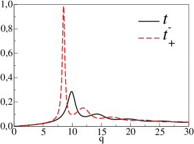
Figure 2: Dwell time eigenvalues for the square barrier, in units of $mL^{2}/\hbar$, for $Q=8$

IV.2 Average dwell time from fluorescence measurements

In this subsection we shall model the measurement of the average dwell time $\tau_{D}=\langle\widehat{T}_{D}\rangle$ of an ultracold atom at a square barrier created by a laser shining perpendicularly to its motion with homogeneous intensity between $0$ and $L$.

Consider a two level system coupled in a spatial region to an off-resonance laser with large detuning, $\Delta\gg\gamma,\Omega$, where $\Delta$ is defined as the laser frequency minus the frequency of the atomic transition, $\gamma$ is the decay constant (inverse lifetime or Einstein’s coefficient), and $\Omega$ is the Rabi frequency.

The amplitude for the atomic ground state up to the first photon detection is governed then by the following effective potential, see Heinzen ; NEMH2003 or Chapter …,

$$V(x)=V_{R}-\mathrm{i}V_{I}=\frac{\hbar\Omega^{2}}{4\Delta}-\mathrm{i}\frac{\hbar\gamma\Omega^{2}}{8\Delta^{2}}\;.$$ (38)

so that the average detection delay (life time of the ground state if the atom at rest is put in the laser-illuminated region) is, see e.g. ME08 , $4\Delta^{2}/\Omega^{2}\gamma$. Whereas $\gamma$ is fixed for the atomic transition, $\Omega$ and $\Delta$ may be controlled experimentally, and the ratio $\Omega^{2}/\Delta$ can always be chosen so that the real part of $V$ remains constant. This still leaves some freedom to fix their exact values which we may use to set the imaginary part. If we do so making sure that at most one fluorescence photon is emitted per atom, i.e., $\tau_{D}\gg 4\Delta^{2}/\Omega^{2}\gamma$, so that the fluorescence signal produced by an atomic ensemble will be proportional to the absorption probability $A$, this signal provides, after calibration to take into the detector solid angle and efficiency, and approximation for the derivative (40) and therefore to the average dwell time for the potential (38) as

$$\tau_{D}\approx\hbar A/(2V_{I})\;.$$ (39)

This follows by integrating $-dN/dt=(2V_{I}/\hbar)\langle\psi(t)|{\chi}_{D}(\widehat{x})|\psi(t)\rangle$ over time, $N$ being the surviving norm, and $A=1-N$ the absorption (fraction of atoms detected). In the limit $V_{I}\to 0$ and for highly monochromatic incidence, the average (stationary) dwell time at the real potential is obtained,

$$\mathsf{T}_{kk}=\lim_{V_{I}\to 0}(\hbar/2)\partial_{V_{I}}A(k)\;,$$ (40)

where $A(k)$ is the total absorption probability for incident wavenumber $k$. The equivalence of this quantity with $(t_{+}(k)+t_{-}(k))/2$ can readily be checked.

Figure 3: Exact average dwell time (solid line) for Cs atoms crossing a square barrier of width 2$\mu$m and height $8.2674\times 10^{3}s^{-1}\hbar$ (in velocity units, $0,28$ cm/s) versus incident velocity. Approximations are calculated with Eq. (39) for $V_{I}=3.307s^{-1}\hbar=V_{1}$ (indistinguishable from the exact result, $\Delta=2500\gamma$, $\Omega=1.57\gamma$), 10 $V_{1}$ (double dotted-dashed line, $\Delta=250\gamma$, $\Omega=0.5\gamma$), $10^{2}V_{1}$ (dashed line, $\Delta=25\gamma$, $\Omega=.16\gamma$), and $10^{3}V_{1}$ (dotted dashed line, $\Delta=2.5\gamma$, $\Omega=0.05\gamma$). The transition is at 852 nm with $\gamma$=33.3$\times 10^{6}$s^-1; $\Delta$ and $\Omega$ are obtained from Eq. (38)

One may think of relaxing the one-photon condition to get a proxy for the dwell time of an individual atom of the ensemble from the photons detected in an idealized one-atom-at-a-time experiment. For $V_{R}$ negligible versus $E$, it could be expected that for some regime this distribution of emitted photons would also be bimodal. For the bimodality to be observed, the characteristic interval between modes ($\hbar/E$, where $E$ is the particle’s energy) should be greater than the characteristic interval between successive emission of fluorescence photons, but these conditions and $\Delta>\gamma$ are not compatible, and similar difficulties are found for on-resonance excitation. A pending task is the application of (deconvolution or operator normalization) techniques which have been successfully applied to the arrival time, at least in theory.

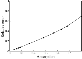
Figure 4: Relative errors, calculated from the maxima of exact and approximate results, $|\tau_{D}(\rm{exact})-\tau_{D}(\rm{approx})|/\tau_{D}(\rm{exact})$, versus the absorption (i.e., detection) probability used to calculate $\tau_{D}(approx)$ at the maximum. Same system as for the previous figure

Figure 3 shows the exact dwell time and approximations for several values of $V_{I}$ calculated for a transition of $Cs$ atoms (the details are in the figure caption). A larger $V_{I}$ implies larger errors but also a stronger signal. In practice the minimal signal requirements will determine the accuracy with which the dwell time can be measured. Figure 4 shows the relative error of the dwell-time maxima versus the corresponding absorption probability. In this figures the beam is monochromatic. We can check the reality of the quantum prediction at hand, differing from the classical one; namely, that for all ingoing waves the quantum mechanical dwell time is bounded, unlike the classical one.

V Some extensions

In this section we present miscellaneous extensions of the previous formalism and results: for bound states, for dwelling into states rather than in a spatial region, and for multiparticle systems.

V.1 The Harmonic oscillator and systems with bound states

If we were to try the direct application of definition (1) to the case of the harmonic oscillator we would soon run into trouble due to divergent integrals. A natural option is to restrict the total time to one period of the system, as follows:

$$\widehat{T}_{D}=\int_{-T/2}^{T/2}\mathrm{d}\tau\,\mathrm{e}^{\mathrm{i}\widehat{H}\tau/\hbar}\chi_{D}(\widehat{x})\,\mathrm{e}^{-\mathrm{i}\widehat{H}\tau/\hbar}\;,$$ (41)

where the Hamiltonian is $\widehat{p}^{\,2}/2m+m\omega^{2}\widehat{x}^{\,2}/2$, and $T=2\pi/\omega$. We can thus write the dwell-time operator, restricted to one period, as

$$\widehat{T}_{D}=T\sum_{n=0}^{\infty}\left\langle n\left|\chi_{D}(\widehat{x})\right|n\right\rangle\left|n\right\rangle\left\langle n\right|\;.$$ (42)

The eigenvalues, $T\left\langle n\left|\chi_{D}(\widehat{x})\right|n\right\rangle$, can be understood as the period times the proportion of that period spent by the particle in the stationary state in the region $D$. This suggests an alternative useful quantity for systems whose Hamiltonian has a purely point spectrum. Define

$$\widehat{\tau}_{D}=\lim_{T\rightarrow\infty}\frac{1}{T}\int_{-T/2}^{T/2}\mathrm{d}\tau\,\mathrm{e}^{\mathrm{i}\widehat{H}\tau/\hbar}\chi_{D}(\widehat{x})\,\mathrm{e}^{-\mathrm{i}\widehat{H}\tau/\hbar}\;.$$ (43)

Let the Hamiltonian be given by

$$\widehat{H}=\sum_{n,\alpha}E_{n}\left|E_{n},\alpha\right\rangle\left\langle E_{n},\alpha\right|\;,$$ (44)

with $\alpha$ a degeneracy index. Then it is easy to compute

$$\widehat{\tau}_{D}=\sum_{n,\alpha,\beta}\left|E_{n},\alpha\right\rangle\left\langle E_{n},\alpha\right|\chi_{D}(\widehat{x})\left|E_{n},\beta\right\rangle\left\langle E_{n},\beta\right|\;,$$ (45)

that is to say, the operator that gives us the fraction of time spent in region $D$ is diagonal in the energy basis, up to degeneracy in energy.

V.2 Times of Residence

The construction above suggests an extension to the time of residence, which is an analogue of the dwell time valid for systems in which the concept of a region in space is not applicable. The question we now purport to answer is the following one: how much time has a system spent in a state $\left|\psi\right\rangle$? Or, alternatively, from time 0 to $T$, what is the proportion of time the system has spent in that state? Let then the projector associated with the state $\left|\psi\right\rangle$ be denoted by $P$, and the unitary evolution operator by $U(t)$. We define the time-of-residence operator as

$$\widehat{\tau}_{\psi}(0;T)=\int_{0}^{T}\mathrm{d}t\,U^{{\dagger}}(t)PU(t)\;.$$

For example S04 , consider a two-level system with Hamiltonian

$$\widehat{H}=\frac{\hbar}{2}\left(\begin{array}[]{cc}0&\Omega\\ \Omega&0\end{array}\right)\;,$$

and the state $\left|\psi\right\rangle=\left(\begin{array}[]{c}1\\ 0\end{array}\right)$. The time of residence gets written as

$$\widehat{\tau}_{\psi}(0;T)=\left(\begin{array}[]{cc}\frac{T}{2}+\frac{1}{2\Omega}\sin\left(\Omega T\right)&\frac{-\mathrm{i}}{2\Omega}\left(1-\cos\left(\Omega T\right)\right)\\ \frac{\mathrm{i}}{2\Omega}\left(1-\cos\left(\Omega T\right)\right)&\frac{T}{2}-\frac{1}{2\Omega}\sin\left(\Omega T\right)\end{array}\right)\;.$$

This entails that the measurement of this quantity would inevitably lead to one of the following two (eigen)values:

$$\tau_{\pm}=\frac{T}{2}\pm\frac{\sin\left(\Omega T/2\right)}{\Omega}\;.$$

The fact that only two values can be obtained in each realization of the experiment, and not a continuous distribution of time of presence in the state $\left|\psi\right\rangle=\left(\begin{array}[]{c}1\\ 0\end{array}\right)$, has been attributed to a predictive character of the measurement involved, as opposed to an observation that extends over time through the coupling with a weakly interacting clocking system S04 .

As a matter of fact, the average time spent by a particle prepared at instant 0 in a generic state ranges from $\tau_{-}$ to $\tau_{+}$ for the eigenstate of $P$. Represent a generic pure or mixed state $\rho$ by a vector in or on the Bloch sphere, $\rho=({1}+\vec{r}\cdot\vec{\sigma})/2$; then the average time of residence in state $\left(\begin{array}[]{c}1\\ 0\end{array}\right)$ over the time interval $[0,T]$ is $T/2+\left[(1-\cos\left(\Omega T\right))r_{y}+\sin\left(\Omega T\right)r_{x}\right]/2\Omega$, which, as stated, ranges over $[\tau_{-},\tau_{+}]$.

It should be noticed that the operator of time of residence from instant 0 to instant $T$ is generically not stationary; for the example at hand we have

$$\left[\widehat{H},\widehat{\tau}_{\psi}(0;T)\right]=\frac{\mathrm{i}\hbar}{2}\left(\begin{array}[]{cc}1-\cos\left(\Omega T\right)&i\sin\left(\Omega T\right)\\ -i\sin\left(\Omega T\right)&-1+\cos\left(\Omega T\right)\end{array}\right)\;.$$

Notice that whenever $T=2n\pi/\Omega$, with $n$ a natural number, the corresponding time of residence does indeed commute with the Hamiltonian; this is in keeping with the expressions of Section V.1.

V.3 Multi-particle systems

The definition (1) admits a straightforward extension to systems of many particles, using the formalism of second quantization, in which we perform the substitution

$$\chi_{D}(\widehat{x})\rightarrow\widehat{n}_{D}=\int_{D}\mathrm{d}x\,\widehat{a}_{x}^{\dagger}\widehat{a}_{x}\,,$$ (46)

where $\widehat{a}_{x}$ is the annihilation operator at point $x$. For free particles, that is to say, for a Hamiltonian of the form

$$\widehat{H}=\int_{-\infty}^{\infty}\mathrm{d}k\,\frac{\hbar^{2}k^{2}}{2m}\widehat{n}_{k}=\int_{-\infty}^{\infty}\mathrm{d}k\,\frac{\hbar^{2}k^{2}}{2m}\widehat{a}_{k}^{\dagger}\widehat{a}_{k}\;,$$ (47)

with $\widehat{a}_{k}$ the operator that annihilates a particle with wavenumber $k$, we can compute the dwell-time operator as

$$\widehat{T}_{D}=\int_{-\infty}^{\infty}\mathrm{d}k\,\frac{mL}{|k|\hbar}\left[\widehat{a}_{k}^{\dagger}\widehat{a}_{k}+\frac{1}{kL}\mathrm{e}^{\mathrm{i}kL}\sin\left({kL}\right)\widehat{a}_{-k}^{\dagger}\widehat{a}_{k}\right]\;.$$ (48)

It is also feasible to write a dwell-time density operator, which for the free case reads

$$\widehat{\Pi}_{\mathrm{a}}(t) = \int_{-\infty}^{\infty}\mathrm{d}k\,\left\{\frac{1}{2}\left[\delta\left(t-t_{+}(k)\right)+\delta\left(t-t_{-}(k)\right)\right]a_{k}^{\dagger}a_{k}\right.$$

$$+\left.\frac{\mathrm{e}^{-\mathrm{i}kL}}{2}\left[\delta\left(t-t_{+}(k)\right)-\delta\left(t-t_{-}(k)\right)\right]a_{k}^{\dagger}a_{-k}\right\}\;.$$

It is easy to see that $\langle\psi|\widehat{\Pi}_{\mathrm{a}}(t)|\psi\rangle$ reduces to the dwell-time density for the one particle marginal wavefunction. The real multiparticle aspect of this construction will only be accessible through dwell time - dwell-time correlation functions, for which a suitable operational interpretation needs to be built.

In addition, we note that for multiparticle systems, the alternative question might be posed, as to what is the time during which a given number of particles $n$ can be found in the region $D$. This naturally leads to the introduction of the dwell-time operator for $n$-particles

$$\widehat{T}_{D}(n) = \int_{-\infty}^{\infty}\mathrm{d}t\widehat{U}^{\dagger}(t)\delta_{\widehat{n}_{D},n}\widehat{U}(t)$$ (49)

$$= \frac{1}{2\pi}\int_{-\infty}^{\infty}\mathrm{d}t\int_{0}^{2\pi}\mathrm{d}\theta\widehat{U}^{\dagger}(t)\mathrm{e}^{\mathrm{i}\theta(\widehat{n}_{D}-n)}\widehat{U}(t)\;,$$

where $\widehat{n}_{D}$ is the density operator restricted to the region $D$, defined in Eq. (46). Letting $\widehat{\rho}$ be the density matrix describing the state of the system, it is convenient to introduce the characteristic function,

$$F(\theta;t)=\mathrm{Tr}[\widehat{\rho}\widehat{U}^{\dagger}(t)\mathrm{e}^{\mathrm{i}\theta\hat{n}_{D}}\widehat{U}(t)]\;,$$ (50)

whose Fourier transform is the atom number distribution in the region $D$ KKS00 ,

$$P_{D}(n,t)=\frac{1}{2\pi}\int_{0}^{2\pi}\mathrm{e}^{-\mathrm{i}n\theta}F(\theta;t)\mathrm{d}\theta\;.$$ (51)

The meaning of $P_{D}(n,t)$ is precisely the probability for $n$ particles to be found in the spatial domain $D$ at time $t$.

Knowledge of the atom-number distribution can be used to compute the average dwell time for different number of particles, namely,

$$\langle\widehat{T}_{D}(n)\rangle=\int_{-\infty}^{\infty}\mathrm{d}t\mathrm{Tr}[\widehat{\rho}(t)\delta_{\widehat{n}_{D},n}]=\int_{-\infty}^{\infty}\mathrm{d}tP_{D}(n,t)\;.$$ (52)

VI Relation to flux-flux correlation functions

This section follows Munoz , and examines a link between the dwell time and flux-flux correlation functions (ffcf) that have been considered mostly in chemical physics to define reaction rates for microcanonical or canonical ensembles MST83 . The motivation for this exercise is to relate the dwell-time distribution, and not just the average value, to other observables.

VI.1 Stationary flux-flux correlation function

Pollak and Miller PoMi-PRL-1984 have shown a connection between the average stationary dwell time and the first moment of a ffcf. They define a quantum microcanonical ffcf $C_{PM}(\tau,k)=\mathrm{Tr}\{\mathrm{Re}\,\widehat{C}_{PM}(\tau,k)\}$ by means of the operator

$$\widehat{C}_{PM}(\tau,k) = 2\pi\hbar[\widehat{J}(x_{2},\tau)\widehat{J}(x_{1},0)+\widehat{J}(x_{1},\tau)\widehat{J}(x_{2},0)$$ (53)

$$- \widehat{J}(x_{1},\tau)\widehat{J}(x_{1},0)-\widehat{J}(x_{2},\tau)\widehat{J}(x_{2},0)]\delta(E-\widehat{H})\;,$$

where $\widehat{J}(x,t)=\mathrm{e}^{\mathrm{i}\widehat{H}t/\hbar}\frac{1}{2m}[\widehat{p}\delta(\widehat{x}-x)+\delta(\widehat{x}-x)\widehat{p}]\mathrm{e}^{-\mathrm{i}\widehat{H}t/\hbar}$ is the quantum mechanical flux operator in the Heisenberg picture, and $\widehat{p}$ and $\widehat{x}$ are the momentum and position operators.

This definition is motivated from classical mechanics: Eq. (53) counts flux correlations of particles entering $D$ through $x_{1}$ ($x_{2}$) and leaving it through $x_{2}$ ($x_{1}$) a time $\tau$ later. Moreover, particles may be reflected and may leave the region $D$ through its entrance point. This is described by the last two terms, where the minus sign compensates for the change of sign of a back-moving flux. Note that these negative terms lead to a self-correlation contribution that diverges for $\tau\to 0$.

We shall first derive the average correlation time and show its equivalence with the average dwell time. We shall only consider positive incident momenta, and define $\widehat{C}^{+}_{PM}$ by substituting $\delta(E-\widehat{H})$ by $\delta^{+}(E-\widehat{H}):=\delta(E-\widehat{H})\Lambda_{+}$, where $\Lambda_{+}$ is the projector onto the subspace of eigenstates of $H$ with positive momentum incidence. By means of the continuity equation,

$$-\frac{\mathrm{d}missing}{\mathrm{d}x}\widehat{J}(x,t)=\frac{\mathrm{d}missing}{\mathrm{d}t}\widehat{\rho}(x,t)\;,$$ (54)

where $\widehat{\rho}(x,t)=\mathrm{e}^{\mathrm{i}\widehat{H}t/\hbar}\delta(\widehat{x}-x)\mathrm{e}^{-\mathrm{i}\widehat{H}t/\hbar}$ is the (Heisenberg) density operator, $\widehat{C}^{+}_{PM}(\tau,k)$ can be written as

$$\widehat{C}^{+}_{PM}(\tau,k)=-2\pi\hbar\left(\frac{\mathrm{d}missing}{\mathrm{d}\tau}\widehat{\chi}_{D}(\tau)\right)\left(\frac{\mathrm{d}missing}{\mathrm{d}t}\widehat{\chi}_{D}(t)\right)_{t=0}\delta^{+}(E-\widehat{H})\;.$$ (55)

By a partial integration and using the Heisenberg equation of motion the first moment of the Pollak-Miller correlation function is given by

$$\mathrm{Tr}\left\{\int_{0}^{\infty}\mathrm{d}\tau\,\tau\widehat{C}^{+}_{PM}(\tau,k)\right\}=\mathrm{Tr}\left\{2\pi\hbar\int_{0}^{\infty}\mathrm{d}\tau\widehat{\chi}_{D}(\tau)\frac{1}{i\hbar}[\widehat{\chi}_{D}(0),\widehat{H}]\delta^{+}(E-\widehat{H})\right\}\;.$$ (56)

Boundary terms of the form $\lim_{\tau\to\infty}\tau^{\gamma}\widehat{\chi}_{D}(\tau),\gamma=0,1,2$, are omitted here and in the following. The contribution of these terms should vanish when an integration over stationary wavefunctions is performed to account for the wavepacket dynamics, as it is done explicitly in the next section. For potential scattering the probability density decays generically as $\tau^{-3}$, which assures a finite dwell-time average, but for free motion it decays as $\tau^{-1}$ MDS95 , making $\tau_{D}$ infinite, unless the momentum wave function vanishes at $k=0$ sufficiently fast as $k$ tends to zero DEMN04 , as we have discussed before.

Writing the commutator explicitly and using the cyclic property of the trace gives

$$\mathrm{Tr}\left\{\int_{0}^{\infty}\mathrm{d}\tau\,\tau\widehat{C}^{+}_{PM}(\tau,k)\right\}$$ (57)

$$= \mathrm{Tr}\left\{2\pi\hbar\int_{0}^{\infty}\mathrm{d}\tau\left(-\frac{\mathrm{d}missing}{\mathrm{d}\tau}\widehat{\chi}_{D}(\tau)\right)\widehat{\chi}_{D}(0)\delta^{+}(E-\widehat{H})\right\}\;,$$

and integration over $\tau$ yields the final result,

$$\mathrm{Tr}\left\{\int_{0}^{\infty}\mathrm{d}\tau\,\tau\widehat{C}^{+}_{PM}(\tau,k)\right\}=2\pi\hbar\mathrm{Tr}\left\{\widehat{\chi}_{D}(0)\delta^{+}(E-\widehat{H})\right\}=\mathsf{T}_{kk}\;.$$ (58)

Expressing the trace in the basis $|\phi_{k}\rangle$ gives back the stationary dwell time of Eq. (6), i.e. the diagonal element of the on-the-energy-shell dwell-time operator, $\mathsf{T}_{kk}$.

The calculation of the average in PoMi-PRL-1984 is different in some respects: The coordinates $x_{1}$ and $x_{2}$ are taken to minus and plus infinity, but it can be carried out for finite values modifying Eq. (8) of PoMi-PRL-1984 accordingly; Formally there are no explicit boundary terms at infinity but a regularization is required in Eq. (16) of PoMi-PRL-1984 , which is justified for wave packets; (c) $\delta(E-\widehat{H})$ is used instead of $\delta^{+}(E-\widehat{H})$. That simply provides an additional contribution for negative momenta parallel to the one obtained here for positive momenta; (d) In our derivation the average correlation time is found to be real directly, even though $\widehat{C}^{+}_{PM}(\tau,k)$ is not selfadjoint, whereas in PoMi-PRL-1984 the real part is taken. (The discussion of the imaginary time average in PoMi-PRL-1984 is based on a modified version of Eq. (53).)

Next, we will show that the second moment of the Pollak-Miller ffcf equals the second moment of $\mathsf{T}$. This was not observed in Ref. PoMi-PRL-1984 . Proceeding in a similar way as above, we start with

$${\cal I}=\mathrm{Tr}\left\{\int_{0}^{\infty}\mathrm{d}\tau\tau^{2}\widehat{C}^{+}_{PM}(\tau,k)\right\}\;.$$ (59)

Integrating by parts twice, neglecting the term at infinity, using Heisenberg’s equation of motion, and the fact that $\phi_{k}$ is an eigenstate of $\widehat{H}$, the real part is

$$\frac{{\cal I}+{\cal I}^{*}}{2}\!=\!\frac{2\pi m}{\hbar k}\!\int_{0}^{\infty}\!\!\!\mathrm{d}\tau\langle\phi_{k}|[\widehat{\chi}_{D}(\tau)\widehat{\chi}_{D}(0)+\widehat{\chi}_{D}(0)\widehat{\chi}_{D}(\tau)]|\phi_{k}\rangle\;.$$ (60)

Introducing resolutions of the identity,

$$\mathrm{Re}{\cal I} = \!\Bigg{\{}\!\!\frac{2\pi m}{\hbar k}\!\!\int_{0}^{\infty}\!\!\!\!\mathrm{d}\tau\!\!\int_{-\infty}^{\infty}\!\!\!\mathrm{d}k^{\prime}\!\!\int_{x_{1}}^{x_{2}}\!\!\!\mathrm{d}x\!\!\int_{x_{1}}^{x_{2}}\!\!\!\mathrm{d}x^{\prime}\mathrm{e}^{\mathrm{i}(E-E^{\prime})\tau/\hbar}\phi_{k}^{*}(x)\phi_{k^{\prime}}(x)\phi_{k^{\prime}}^{*}(x^{\prime})\phi_{k}(x^{\prime})\!\Bigg{\}}$$ (61)

$$+ c.c.\;,$$

where $c.c$ means complex conjugate. Making the changes $\tau\to-\tau$ and $x,x^{\prime}\to x^{\prime},x$ in the $c.c$-term, it takes the same form as the first one, but with the time integral from $-\infty$ to $0$. Adding the two terms, the $\tau$-integral provides an energy delta function that can be separated into two deltas which select $k^{\prime}=\pm k$ to arrive at

$$\mathrm{Tr}\left\{\mathrm{Re}\int_{0}^{\infty}\mathrm{d}\tau\,\tau^{2}\widehat{C}^{+}_{PM}(\tau,k)\right\} = \frac{4\pi^{2}m^{2}}{\hbar^{2}k^{2}}\Bigg{[}\Big{(}\int_{x_{1}}^{x_{2}}\mathrm{d}x\,|\phi_{k}(x)|^{2}\Big{)}^{2}$$ (62)

$$+ \Big{|}\int_{x_{1}}^{x_{2}}\!\mathrm{d}x\,\phi_{k}^{*}(x)\phi_{-k}(x)\Big{|}^{2}\Bigg{]}=(\mathsf{T}^{2})_{kk}\;.$$

In other words, the relation between dwell times and flux-flux correlation functions goes beyond average values and $C^{+}_{PM}(\tau,k)$ includes quantum features of the dwell time: note that the first summand in Eq. (62) is nothing but $(\mathsf{T}_{kk})^{2}$, whereas the second summand is positive, which allows for a non-zero on-the-energy shell dwell-time variance $(\mathsf{T}^{2})_{kk}-(\mathsf{T}_{kk})^{2}$. We insist that the stationary state considered has positive momentum, $\phi_{k}(x)$, $k>0$, but this second term implies the degenerate partner $\phi_{-k}(x)$ as well, and is generically non-zero.

We shall see in the next section with a more general approach, that these connections do not hold for higher moments.

VI.2 Time-dependent flux-flux correlation function

A time-dependent version of the above flux-flux correlation function can be defined in terms of the operator

$$\widehat{C}(\tau) = \int_{-\infty}^{\infty}\mathrm{d}t\,\bigl{[}\widehat{J}(x_{2},t+\tau)\widehat{J}(x_{1},t)+\widehat{J}(x_{1},t+\tau)\widehat{J}(x_{2},t)$$ (63)

$$- \widehat{J}(x_{1},t+\tau)\widehat{J}(x_{1},t)-\widehat{J}(x_{2},t+\tau)\widehat{J}(x_{2},t)\bigr{]}\;,$$

which leads to the flux-flux correlation function

$$C(\tau)=\langle\mathrm{Re}\,\widehat{C}(\tau)\rangle_{\psi}\;,$$ (64)

where the real part is taken to symmetrize the non-selfadjoint operator $\widehat{C}(\tau)$ as before.

As in the stationary case, Eq. (64) counts flux correlations of particles entering $D$ through $x_{1}$ or $x_{2}$ at a time $t$ and leaving it either through $x_{1}$ or $x_{2}$ a time $\tau$ later. Moreover we integrate over the entrance time $t$. It can be shown that the first moment of the classical version of Eq. (63), where $\widehat{J}$ is replaced by the classical dynamical variable of the flux, gives the average of the classical dwell time.

As in Eq. (55), we may rewrite $\widehat{C}(\tau)$ as

$$\widehat{C}(\tau)=-\int_{-\infty}^{\infty}\mathrm{d}t\frac{\mathrm{d}missing}{\mathrm{d}\tau}\widehat{\chi}_{D}(\widehat{x},t+\tau)\frac{\mathrm{d}missing}{\mathrm{d}t}\widehat{\chi}_{D}(\widehat{x},t)\;.$$ (65)

From here we note that the ffcf $C(\tau)$ is not normalized,

$$\int_{0}^{\infty}\mathrm{d}\tau\,\widehat{C}(\tau)=\int_{-\infty}^{\infty}\mathrm{d}t\,\widehat{\chi}_{D}(t)\frac{\mathrm{d}missing}{\mathrm{d}t}\widehat{\chi}_{D}(t)=0\;,$$ (66)

as a result of the self-correlation.

Next we derive the average of the time-dependent correlation function. With a partial integration one finds

$$\int_{0}^{\infty}\mathrm{d}\tau\,\tau\widehat{C}(\tau)=\int_{-\infty}^{\infty}\!\mathrm{d}t\int_{0}^{\infty}\!\mathrm{d}\tau\,\widehat{\chi}_{D}(\widehat{x},t+\tau)\frac{\mathrm{d}missing}{\mathrm{d}t}\widehat{\chi}_{D}(\widehat{x},t)\;.$$

A second partial integration with respect to $t$, replacing $\mathrm{d}/\mathrm{d}t$ by $\mathrm{d}/\mathrm{d}\tau$ and integrating over $\tau$ gives

$$\int_{0}^{\infty}\mathrm{d}\tau\,\tau\widehat{C}(\tau)=\int_{-\infty}^{\infty}\!\mathrm{d}t\,\widehat{\chi}_{D}^{2}(\widehat{x},t)=\int_{-\infty}^{\infty}\mathrm{d}t\,\widehat{\chi}_{D}(\widehat{x},t)=\widehat{T}_{D}\;,$$ (67)

where $\widehat{\chi}_{D}^{2}=\widehat{\chi}_{D}$ has been used. Eq. (67) generalizes the result of Pollak and Miller to time-dependent dwell times.

A similar calculation can be performed for the second moment of $C(\tau)$. After three partial integrations with vanishing boundary contributions to get rid of the factor $\tau^{2}$ one obtains

$$\int_{0}^{\infty}\mathrm{d}\tau\,\tau^{2}\widehat{C}(\tau)=2\int_{-\infty}^{\infty}\!\mathrm{d}t\int_{0}^{\infty}\mathrm{d}\tau\,\widehat{\chi}_{D}(\widehat{x},t+\tau)\widehat{\chi}_{D}(\widehat{x},t)\;.$$

Making the substitutions $t+\tau\to t$ and $\tau\to-\tau$ in the complex conjugated term, we find

$$\mathrm{Re}\int_{0}^{\infty}\mathrm{d}\tau\,\tau^{2}\widehat{C}(\tau)=\widehat{T}_{D}^{2}\;.$$ (68)

VI.3 Example: free motion

For a stationary flux of freely-moving particles with energy $E_{k}$, $k>0$, described by $\phi_{k}(x)=\langle x|k\rangle=(2\pi)^{-1/2}\mathrm{e}^{\mathrm{i}kx}$, the first three moments of the ideal dwell-time distribution on the energy shell are given by

$$\mathsf{T}_{kk} = \frac{mL}{\hbar k}\;,$$ (69)

$$(\mathsf{T}^{2})_{kk} = \frac{m^{2}L^{2}}{\hbar^{2}k^{2}}\left(1+\frac{\sin^{2}(kL)}{k^{2}L^{2}}\right)\;,$$ (70)

$$(\mathsf{T}^{3})_{kk} = \frac{m^{3}L^{3}}{\hbar^{3}k^{3}}\left(1+3\frac{\sin^{2}(kL)}{k^{2}L^{2}}\right)\;.$$ (71)

As proved above, the first two moments agree with the corresponding moments of the Pollak-Miller ffcf, but for the third moment we obtain instead

$$\mathrm{Tr}\left\{\mathrm{Re}\int_{0}^{\infty}\mathrm{d}\tau\,\tau^{3}\widehat{C}^{+}_{PM}(\tau,k)\right\}=\frac{m^{3}L^{3}}{\hbar^{3}k^{3}}\left[1-\frac{3[1+\cos^{2}(kL)]}{k^{2}L^{2}}+\frac{3\sin(2kL)}{L^{3}k^{3}}\right]\;.$$ (72)

In Fig. 5 the first three moments are compared. The agreement between $(\mathsf{T}^{3})_{kk}$ and Eq. (72) is very good for large values of $k$, but they clearly differ for small $k$. Nevertheless, the agreement of the first two moments suggests a similar behavior of $\Pi(\tau)$ and $C(\tau)$.

To calculate $\Pi_{\psi}(\tau)$ for a wavefunction $\widetilde{\psi}(k):=\langle k|\psi\rangle$ with only positive momentum components we use Eq. (11) and the explicit forms of the eigenvectors, Eq. (14) and eigenvalues $t_{\pm}$, Eq. (15),

$$\Pi_{\psi}(\tau)=\frac{1}{2}\sum_{j}\sum_{\gamma=\pm}\frac{|\widetilde{\psi}(k_{j}^{\gamma}(\tau))|^{2}}{|F^{\prime}_{\gamma}(k_{j}^{\gamma}(\tau))|}\;,$$ (73)

where the $j$-sum is over the solutions $k_{j}^{\gamma}(\tau)$ of the equation $F_{\gamma}(k)\equiv t_{\gamma}(k)-\tau=0$ and the derivative is with respect to $k$.

We use the following wavefunction charac ,

$$\widetilde{\psi}(k)={\cal N}(1-\mathrm{e}^{-\alpha k^{2}})\,\mathrm{e}^{-(k-k_{0})^{2}/[4(\Delta k)^{2}]}\mathrm{e}^{-\mathrm{i}kx_{0}}\Theta(k)\;,$$ (74)

where ${\cal N}$ is the normalization constant and $\Theta(k)$ the step function. For the free flux-flux correlation function we write

$$C(\tau)=\mathrm{Re}\int_{0}^{\infty}\mathrm{d}k\int_{0}^{\infty}\mathrm{d}k^{\prime}\,\widetilde{\psi}^{*}(k)\widetilde{\psi}(k^{\prime})\langle k|\widehat{C}(\tau)|k^{\prime}\rangle\;,$$ (75)

and $C_{kk^{\prime}}(\tau)=\langle k|\widehat{C}(\tau)|k^{\prime}\rangle$ in the free case

$$C_{kk^{\prime}}(\tau)=\frac{m}{2\pi\hbar k}\delta(k-k^{\prime})\frac{\mathrm{d}^{2}}{\mathrm{d}\tau^{2}}\Big{[}2g(\hbar k\tau/m)-g(\hbar k\tau/m-L)-g(\hbar k\tau/m+L)\Big{]}\;,$$ (76)

where

$$g(x)=-2\mathrm{e}^{\mathrm{i}mx^{2}/(2\hbar\tau)}\left(\frac{\mathrm{i}\pi\hbar\tau}{2m}\right)^{1/2}+\mathrm{i}\pi x\,\mathrm{erfi}\left(\sqrt{\frac{\mathrm{i}m}{2\hbar\tau}}\,x\right)\;.$$ (77)

The result is shown in Fig. 6. The ffcf shows a hump around the mean dwell time but it oscillates for small $\tau$ and diverges for $\tau\to 0$. As discussed above, this is due to the self-correlation contribution of wavepackets which are at $x_{1}$ or $x_{2}$ at the times $t$ and $t+\tau$ without changing the direction of motion in between. A similar feature has been observed in a traversal-time distribution derived by means of a path integral approach Fertig-PRL-1990 .

In contrast, $\Pi_{\psi}(\tau)$ behaves regularly for $\tau\to 0$, but shows peaks in the region of the hump. This is because the denominator of Eq. (73) becomes zero if the slope of the eigenvalues $t_{\pm}(k)$ is zero, which occurs at every crossing of $t_{+}(k)$ and $t_{-}(k)$.

The distribution $\pi_{\psi}(\tau)$, see Eq. (27), is also computed: it agrees with $C(\tau)$ in the region near the average dwell time and it tends to zero for $\tau\to 0$. However, it does not show the resonance peaks of $\Pi_{\psi}(\tau)$.

In absence of a direct dwell-time measurement, the physical significance $\widehat{T}_{D}$ and $\widehat{t}_{D}$ depends on their relation to other observables. The present results indicate that the second moment of the flux-flux correlation function is related to the former and not to the later, providing indirect support for the physical relevance of the dwell-time resonance peaks, but other observables could behave differently.

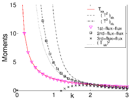
Figure 5: Comparison of the first three moments: $\mathsf{T}_{kk}$, $(\mathsf{T}^{2})_{kk}$ and $(\mathsf{T}^{3})_{kk}$ (dotted-dashed line) with the corresponding moments of the flux-flux correlation function, for a free-motion stationary state with fixed $k$. $(\mathsf{T}_{kk})^{2}$ is also shown (dotted line). $\hbar=m=1$ and $L=2$

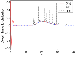
Figure 6: Comparison of dwell-time distribution $\Pi(\tau)$ (dashed line) and flux-flux correlation function $C(\tau)$ (solid line) for the freely moving wave packet (74). Furthermore, the alternative free-motion dwell-time distribution $\pi(\tau)$, Eq. (27), is plotted (circles). We set $\hbar=m=1$ and $|x_{0}|$ large enough to avoid overlap of the initial state with the space region $D=[0,45]$. $k_{0}=2$, $\Delta k=0.4$, and $\alpha=0.5$

VI.4 Approximations

While the previous results bring dwell-time information closer to experimental realization, the difficulty is translated onto the measurement of the ffcf, not necessarily an easy task. A simple approximation is to substitute the expectation of the product of two flux operators by the product of their expectation values, which are the current densities. Using the wave packet of Eq. (74), we have compared the times obtained with the full expression (64) and with this approximation in Fig. 7. The two results approach each other as $\Delta_{k}\to 0$, also by increasing $L$ and/or $k_{0}$.

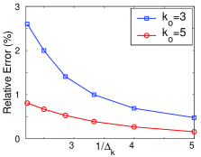
Figure 7: Comparison of the relative error of $\langle\widehat{T}_{D}^{2}\rangle$ using the approximation ${C_{0}}(\tau)$ instead of $C(\tau)$ for free motion. $\alpha=0.5$, $\hbar=m=1$ and $L=100$

The exact result can be approached systematically, still making use of ordinary current densities, as follows: First decompose $\widehat{J}(x_{i},t+\tau)\widehat{J}(x_{j},t)$ by means of

$$\widehat{1} = \widehat{P}+\widehat{Q}\;,$$ (78)

$$\widehat{P} = |\psi\rangle\langle\psi|\;,$$ (79)

so that

$$\widehat{J}(x_{i},t+\tau)\widehat{J}(x_{j},t)=\widehat{J}(x_{i},t+\tau)(|\psi\rangle\langle\psi|+\widehat{Q})\widehat{J}(x_{j},t)\;.$$ (80)

It is useful to decompose $\widehat{Q}$ further in terms of a basis of states orthogonal to $|\psi\rangle$ and to each other, $\{|\psi_{j}^{Q}\rangle\}$,

$$\widehat{Q}=\sum_{j}|\psi_{j}^{Q}\rangle\langle\psi_{j}^{Q}|\;,$$ (81)

that could be generated by means of a Gram-Schmidt orthogonalization procedure. Now we can split Eq. (63),

$$\widehat{C}(\tau)=\widehat{C}_{0}(\tau)+\widehat{C}_{1}(\tau)\;,$$ (82)

where $\widehat{C}_{0}(\tau)$ has the structure of $\widehat{C}$, but with $P$ inserted between the two flux operators in each of the four terms. Similarly $\widehat{C}_{1}(\tau)$ has $Q$ inserted and can be itself decomposed using Eq. (81).

We define $C(\tau)=C_{0}(\tau)+C_{1}(\tau)$ by taking the real real part of $\langle\psi|\widehat{C}_{0}(\tau)+\widehat{C}_{1}(\tau)|\psi\rangle$. $C_{0}$ is the zeroth order approximation discussed before and only involves ordinary, measurable current densities DEHM2002 . The non-diagonal terms from $C_{1}$, $\langle\psi|\widehat{J}(x_{i},t)|\psi_{j}^{Q}\rangle\langle\psi_{j}^{Q}|\widehat{J}(x_{j},t+\tau)|\psi\rangle$ can also be related to diagonal elements of $\widehat{J}$ by means of the auxiliary states

$$|\psi_{1}\rangle = |\psi\rangle+|\psi_{j}^{Q}\rangle\;,$$

$$|\psi_{2}\rangle = |\psi\rangle+\mathrm{i}|\psi_{j}^{Q}\rangle\;,$$

$$|\psi_{3}\rangle = |\psi\rangle-\mathrm{i}|\psi_{j}^{Q}\rangle\;,$$ (83)

since

$$\langle\psi|\widehat{J}(x,t)|\psi_{j}^{Q}\rangle = \frac{1}{2}\langle\psi_{1}|\widehat{J}(x,t)|\psi_{1}\rangle-\frac{1}{4}\langle\psi_{2}|\widehat{J}(x,t)|\psi_{2}\rangle$$ (84)

$$- \frac{1}{4}\langle\psi_{3}|\widehat{J}(x,t)|\psi_{3}\rangle+\frac{\mathrm{i}}{4}\langle\psi_{3}|\widehat{J}(x,t)|\psi_{3}\rangle$$

$$- \frac{\mathrm{i}}{4}\langle\psi_{2}|\widehat{J}(x,t)|\psi_{2}\rangle\;.$$

VII Final comments

The quantum dwell-time distribution of a particle in a spatial region, and its second moment present non-classical features even for the simplest case of a freely moving particle, such as bimodality (due to two different eigenvalues for the same energy) with the strongest deviations from classical behavior occurring for de Broglie wavelengths of the order or larger than the region width. Progress in ultracold atom manipulation makes plausible the observation of these effects, and motivates further effort to achieve an elusive direct measurement of the dwell times, or to link the distribution and its moments to other observables. We have in this regard pointed out that the flux-flux correlation function provides access to the second moment. The potential impact in cold atom time-frequency metrology sei07 ; mou07 , and other fields in which the dwell time plays a prominent role (such as conductivity Bu , or chaos) remains an open question.

References

• (1) D. Alonso, R. Sala Mayato, J. G. Muga, Phys. Rev. A 67, 032105 (2003). This paper states incorrectly that the distributions for $\widehat{T}_{D}$ and $\widehat{t}_{D}$ coincide, see the last two equations in it and the related paragraph.
• (2) A. Baz’, Sov. J. Nucl. Phys. 4, 182 (1967)
• (3) S. Boonchui, V. Sa-yakanit, Phys. Rev. 77, 044101 (2008)
• (4) C. Bracher, J. Phys. B: At. Mol. Opt. Phys. 30, 2717 (1997)
• (5) S. Brouard, R. Sala, J.G. Muga, Phys. Rev. A 49, 4312 (1994)
• (6) M. Büttiker, Phys. Rev. B 27, 6178 (1983)
• (7) M. Büttiker, H. Thomas, A. Pr$\hat{e}$tre, Phys. Lett. A 180, 364 (1993)
• (8) C.A.A. de Carvalho, H.M. Nussenzveig, Phys. Rep. 364, 83 (2002)
• (9) J.A. Damborenea, I.L. Egusquiza, G.C. Hegerfeldt, J.G. Muga, Phys. Rev. A 66, 052104 (2002)
• (10) J.A. Damborenea, I.L. Egusquiza, J.G. Muga, J. Am. Phys. 70, 738 (2002)
• (11) J.A. Damborenea, I.L. Egusquiza, J.G. Muga, B. Navarro, arXiv:quant-ph/0403081 (2004)
• (12) I.L. Egusquiza, J.G. Muga, A.D. Baute: in Time in Quantum Mechanics, Vol. 1, ed. by J.G. Muga, R. Sala and I. Egusquiza ( Springer, Berlin, 2008), Chapter 10
• (13) H. Ekstein, A.J.F. Siegert, Ann. Phys. 68, 509 (1971)
• (14) H.A. Fertig, Phys. Rev. Lett. 65, 2321 (1990)
• (15) M.L. Goldberger, K.M. Watson, Collision theory (Krieger, Huntington, 1975)
• (16) R. Golub, S. Felber, R. Gähler, E. Gutsmiedl, Phys. Lett. A 148, 27 (1990)
• (17) E.H. Hauge, J.A. Støvneng, Rev. Mod. Phys. 61, 917 (1989)
• (18) Z. Huang, C.M. Wang, J. Phys.: Cond. Matt 3, 5915 (1991)
• (19) W. Jaworski, D.M. Wardlaw, Phys. Rev. A 37, 2843 (1988)
• (20) W. Jaworski, D.M. Wardlaw, Phys. Rev. A 40, 6210 (1989)
• (21) N.G. Kelkar, Phys. Rev. Lett. 99, 210403 (2007)
• (22) V.V. Kocharovsky, Vl.V. Kocharovsky, M.O. Scully, Phys. Rev. Lett. 84, 2306 (2000)
• (23) R. Landauer, T. Martin, Rev. Mod. Phys. 66, 217 (1994)
• (24) C.R. Leavens, W.R. McKinnon, Phys. Lett. A 194, 12 (1994)
• (25) H. Lewenkopf R.O. Vallejos, Phys. Rev. E 70, 036214 (2004)
• (26) W.H. Miller, S.D. Schwartz, J.W. Tromp, J. Chem. Phys. 79, 4889 (1983)
• (27) J.D. Miller, R.A. Cline, D.J. Heinzen, Phys. Rev. A 47 (1993) R4567
• (28) S.V. Mousavi, A. del Campo, I. Lizuain, J.G. Muga, Phys. Rev. A 76, 033607 (2007)
• (29) J. G. Muga in Time in Quantum Mechanics, Vol. 1, ed. by J.G. Muga, R. Sala and I. Egusquiza ( Springer, Berlin, 2008), Chapter 2
• (30) J.G. Muga, G.R. Leavens, Phys. Rep. 338, 353 (2000)
• (31) J.G. Muga, D. Wardlaw, Phys. Rev. E 51, 5377 (1995)
• (32) J.G. Muga, S. Brouard, R. Sala, Phys. Lett. A 167, 24 (1992)
• (33) J.G. Muga, S. Brouard, R. Sala, J. Phys.: Cond. Matt. 4, L579 (1992)
• (34) J.G. Muga, V. Delgado, R.F. Snider, Phys. Rev. 52, 16381 (1995)
• (35) J.G. Muga, R. Sala Mayato, I.L. Egusquiza (eds.), Time in Quantum Mechanics - Vol. 1, (Springer, Berlin, 2008).
• (36) J. G. Muga, J. Echanobe, A. del Campo, I Lizuain, J. Phys. B: At. Mol. Opt. Phys. 41, 175501 (2008)
• (37) J. Mu oz, D. Seidel, J.G. Muga, Phys. Rev. A (2009)
• (38) B. Navarro B, I.L. Egusquiza, J.G. Muga, G.C. Hegerfeldt, J. Phys. B: At. Mol. Opt. Phys. 36 3899 (2003)
• (39) J.P. Palao, J.G. Muga, S. Brouard, A. Jadczyk, Phys. Lett. A 233, 227 (1997)
• (40) E. Pollak, W.H. Miller, Phys. Rev. Lett. 53, 115 (1984)
• (41) A. Ruschhaupt, Phys. Lett. A 250, 249 (1998)
• (42) A. Ruschhaupt, J.A. Damborenea, B. Navarro, J.G. Muga, G.C. Hegerfeldt, Europhys. Lett. 67, 1 (2004)
• (43) V. Rybachenko, Sov. J. Nucl. Phys. 5, 635 (1967)
• (44) D. Seidel, J.G. Muga, Eur. Phys. J. D 41, 71 (2007)
• (45) F. Smith, Phys. Rev. 118, 349 (1960)
• (46) D. Sokolovski, Phys. Rev. A 66, 032107 (2002)
• (47) D. Sokolovski, Proc. R. Soc. Lond. A 460, 1505 (2004)
• (48) D. Sokolovski, Phys. Rev. A 76, 042125 (2007)
• (49) D. Sokolovski in Time in Quantum Mechanics, Vol. 1, ed. by J.G. Muga, R. Sala and I. Egusquiza ( Springer, Berlin, 2008), Chapter 7
• (50) D. Sokolovski, J.N.L. Connor, Phys. Rev. A 44, 1500 (1991)
• (51) H.G. Winful, Phys. Rep. 436, 1 (2006)
• (52) N. Yamada, Phys. Rev. Lett. 93, 170401 (2004)