A Theoretical Study on an Optical Switch Using Interfered Evanescent Light

Abstract

In an optical configuration consisting of a flat plate of vacuum between upper and lower spaces of uniform dielectric regions of $n>1$, we have calculated two output light intensities for two input lights from the Maxwell’s equations as functions of the incision angle, a light intensity ratio, a phase difference of the two input lights, and a thickness of the vacuum layer, where the two input lights come from upper and lower dielectric regions with the same incision angles, and one of the output light goes into upper dielectric and the other goes into lower dielectric. We have found that, when evanescent lights exist at the upper and lower boundary and interfere each other, there is one set of incision angles and phase differences for any combination of an input light ratio and a thickness of the vacuum layer where one of output lights becomes zero. This finding will possibly lead to an innovative optical switch with which an optical output light can be switched on and off with a control light with an intensity much lower than that of the output light.

I Introduction

In the present wired tele-communication, the optical fiber using an infrared light with wavelength around 1500 nm is playing the main role, but the signal processing at both ends of the transmission optical fiber is done with electronics. That means there are optoelectronic and electro-optic converter circuits between optical fibers and electronic circuits. In order to avoid a demerit of electronic circuits that they are vulnerable of electro-magnetic noise and also to simplify devices by eliminating optoelectronic and electro-optic converters, a purely optical signal processing device represented by optical switches has long been desired.

Optical waveguides are utilized in optical communication devices as star-couplers and array waveguide gratings (AWG) to add or to divide optical signals. A star-coupler is a device to divide the energy of an optical signal carried by the core of an optical fiber into several output optical signals. The AWG is used for a filter using a characteristic that multiple optical signals interfere each other in a small space of a optical waveguide circuit.

Figure 1: An optical switch of the present article

An optical splitter and an optical coupler are made of an optical fiber or an optical waveguide. They can be the same device by exchanging their inputs and outputs of lights. To divide or add optical signals, the device can be an optical waveguide with a geometrical branch shape or two parallel optical fibers. When two optical fibers are located in parallel and very close to each other, the energy of an optical signal is transferred from an optical fiber to other fiber. As the optical switching elements, semi-conductors or ceramics having characteristics of changing their optical properties such as refractive index with electric field, magnetic field, or temperature have been developed and utilized. Such devices as the one composed of a lattice of optical waveguides with optical switching materials buried at each cross point of the lattice are proposed and some of them have been realized.

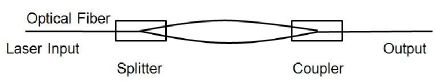
Figure 2: Mach-Zehnder Circuit

The evanescent light is a kind of light existing on places such as the back side of a total reflection prism within a very small area, typically within a distance of one wavelength. The evanescent light can be developed from the Maxwell’s equations, but it is only a decade ago that the evanescent light became one of major research subjects. The evanescent light has already been utilized probably based on the empirical findings. That is the divider or coupler made of two parallel optical fibers mentioned above. The evanescent light appears on the surface of the input optical fiber and the energy of light moves into the output optical fiber running close by and in parallel. The amount of light energy transferred to the output fiber depends on the gap between two fibers and the length of these two fibers running together in parallel. The ratio of light energy splitting/coupling can be controlled in the manufacturing. This type of a coupler/splitter is produced with carefully adjusting the gap and length watching the intensity of output light. The produced coupler/splitter has two input optical fibers and two output fibers, and that is one of the simplest example of the four terminal circuits as shown in Fig.1.

An example of a coupler/splitter application is the Mach-Zehnder interferometer which is composed of a 50:50 splitter and a 50:50 coupler with two transmission lines between them, as shown in Fig.2. The splitter and coupler in this case are the same configuration as the four terminal circuit explained above but one of four terminals is neglected or the ratio of light energy to one of four terminals is designed to be zero.  The Mach-Zehnder interferometer can also be made by dielectric optical waveguides.

A coherent light injected to the input of the Mach-Zehnder interferometer is divided equally to two transmission lines and when the two transmission lines are same, lights from the two transmission lines are simply added at the coupler and the same light as the input light goes out. When there occurs a phase difference between two transmission lines between the splitter and the coupler, sum of two lights having phase difference is given to the output terminal. If the phase difference is $\pi$, then the output is zero. Therefore, a light switch or a light modulator can be made by using a light phase controller and a Mach-Zehnder interferometer.

In this paper, we propose a new type of optical switch which is expressed by a four terminal circuit as Fig.1. Two lights having a particular relation between them injected into two input terminals produce their evanescent lights and through interference of the evanescent lights in this new device, the two output lights are switched on and off. We have theoretically studied the mechanism by solving the Maxwell’s equations including evanescent lights.

Figure 3: A theoretical model

II Calculation model and contents of this paper

As shown in Fig.3, we set a calculation model consisting of three regions. Region 1 : $z>d/2$, refractive index $n$, region 2 : $-d/2<z<d/2$, vacuum (refractive index 1), and region 3 : $z<-d/2$, refractive index $n$. A light (I1) with a vacuum wave length $\lambda$ and intensity 1 is injected from region 1 with an injection angle $\theta$, and another light (I2) of same wave length with intensity $\alpha$ is injected from region 3 with the same injection angle $\theta$. I2 has a phase difference (delay) $\eta$ relative to I1 when the two lights arrive at the boundary at the same $x$.

In section III, we have calculated the ratio $\overline{R}$ of an output light (O1) intensity to an input light (I1) intensity, both in the region 1, with $\theta$ less than the critical angle where refraction lights propagate in region 2. We have also calculated $\overline{R}$ with $\theta$ larger than the critical angle in section IV taking the evanescent light in region 2 into account. In section V, we have discussed the conditions where $\overline{R}=0$ based on the results attained in sections III and IV. The conditions for $\overline{T}=0$, the condition for the output light into the region 3 being zero, is not discussed because the total energy of the input lights (I1 + I2) is conserved to that of the output lights (O1 + O2) in the present model, and the condition is clearly $\overline{R}+\overline{T}=1+\alpha$.

III Output intensity when the injection angle is less than the critical angle

Because no electric charge and no electric current exist in the model of Fig.3, the Maxwell’s equations to be solved are:

$$\nabla\times{\bf E}+\partial_{t}{\bf B} ={\bf 0},$$ (1a)

$$\nabla\cdot{\bf B} =0,$$ (1b)

$$\nabla\times{\bf H}-\partial_{t}{\bf D} ={\bf 0},$$ (1c)

$$\nabla\cdot{\bf D} =0,$$ (1d)

where $\partial_{t}$ means $\frac{\partial}{\partial t}$, ${\bf E}$ and ${\bf D}$ are the electric field vector and electric flux vector, respectively, and ${\bf H}$ and ${\bf B}$ are the magnetic field vector and magnetic flux vector, respectively. Using the dielectric constant $\varepsilon$ and the magnetic permeability $\mu$, the ${\bf D}$ and ${\bf B}$ are expressed as:

$${\bf D} =\varepsilon{\bf E}, {\bf B} =\mu{\bf H}.$$ (2)

In the present calculation, we set $\mu=1$ in all the regions.

Figure 4: definition of parameters

In general, equations (1a) and (1b) indicate that there exist a scalar potential $f$ and a vector potential ${\bf A}$ which fit to

$${\bf E} =-\nabla f-\partial_{t}{\bf A},$$ (3)

$${\bf B} =\nabla\times{\bf A},$$ (4)

and for a gauge transformation below using any scalar function $g$:

$${\bf A} \rightarrow{\bf A}+\nabla g,$$ (5)

$$f \rightarrow f-\partial_{t}g,$$ (6)

${\bf E}$ and ${\bf B}$ are invariant Jackson ; Berkeley .

Because we are solving a reflection and refraction problem, we take the gauge transformation above and particularly we take the Lorentz gauge of:

$$\nabla\cdot{\bf A} =0, f =0.$$ (7)

Then we have expressed the incision light and the reflection light in the region 1 as below using the vector potential:

$${\bf A}^{1} =\frac{-1}{i\omega}\begin{pmatrix}A^{1}_{TM}\cos\theta\\ A^{1}_{TE}\\ A^{1}_{TM}\sin\theta\end{pmatrix}e^{i\left(\omega t-n\frac{\sin\theta x-\cos\theta z}{\lambdabar}\right)},$$ (8)

$${\bf A}^{R} =\frac{-1}{i\omega}\begin{pmatrix}A^{R}_{TM}\cos\theta\\ A^{R}_{TE}\\ -A^{R}_{TM}\sin\theta\end{pmatrix}e^{i\left(\omega t-n\frac{\sin\theta x+\cos\theta z}{\lambdabar}\right)}.$$ (9)

Similarly, we have expressed those in the region 2 as:

$${\bf A}^{(2,1)} =\frac{-1}{i\omega}\begin{pmatrix}A^{(2,1)}_{TM}\cos\varphi\\ A^{(2,1)}_{TE}\\ A^{(2,1)}_{TM}\sin\varphi\end{pmatrix}e^{i\left(\omega t-\frac{\sin\varphi x-\cos\varphi z}{\lambdabar}\right)},$$ (10)

$${\bf A}^{(2,2)} =\frac{-1}{i\omega}\begin{pmatrix}A^{(2,2)}_{TM}\cos\varphi\\ A^{(2,2)}_{TE}\\ -A^{(2,2)}_{TM}\sin\varphi\end{pmatrix}e^{i\left(\omega t-\frac{\sin\varphi x+\cos\varphi z}{\lambdabar}\right)},$$ (11)

and we have expressed those in the region 3 as:

$${\bf A}^{\alpha} =\frac{-1}{i\omega}\begin{pmatrix}A^{\alpha}_{TM}\cos\theta\\ A^{\alpha}_{TE}\\ A^{\alpha}_{TM}\sin\theta\end{pmatrix}e^{i\left(\omega t-n\frac{\sin\theta x-\cos\theta z}{\lambdabar}\right)},$$ (12)

$${\bf A}^{R} =\frac{-1}{i\omega}\begin{pmatrix}A^{T}_{TM}\cos\theta\\ A^{T}_{TE}\\ -A^{T}_{TM}\sin\theta\end{pmatrix}e^{i\left(\omega t-n\frac{\sin\theta x+\cos\theta z}{\lambdabar}\right)}.$$ (13)

Here, $\omega,\lambdabar$ and $n$ in equations (8)-(13) are angular frequency, $\frac{\lambda}{2\pi}$ of light, and refractive index of region 1 and 3, respectively.

Equations (8)-(13) satisfy the condition of Lorentz gauge (7), and variables with suffix $TM$ are for the TM mode and those with suffix $TE$ are for the TE mode.

The wave equation of the vector potential:

$$\frac{1}{c^{2}}\partial^{2}_{t}{\bf A}-\nabla^{2}{\bf A}=0.$$ (14)

is derived using the Maxwell’s equations (1), the relation between field and flux (2), the relation between the vector potential ${\bf A}$ and the electric field ${\bf E}$ (3), the relation between vector potential and magnetic flux ${\bf B}$ (4), and also the relation between the light velocity $c$ and the dielectric constant $\varepsilon$ and the magnetic permeability $\mu$

$$c^{2}=\frac{1}{\varepsilon\mu},$$ (15)

where $\mu=1$ in the present study.

Therefore, the vector potentials in each region satisfy the dispersion relations:

$$\frac{\omega^{2}}{c_{1}^{2}}=\frac{n^{2}}{{\lambdabar}^{2}}, ~{}\hskip 20.00003pt\text{regions 1 and 3},$$ (16)

$$\frac{\omega^{2}}{c^{2}}=\frac{1}{{\lambdabar}^{2}}, ~{}\hskip 20.00003pt\text{region 2},$$ (17)

where $c_{1}$ is the light velocity in regions 1 and 3, $c$ is the light velocity in vacuum or region 2 and $\lambda$ is the wave-length in vacuum.

From equations (3), (4), (8)-(13), we have derived the electric field and magnetic fields in region 1 as:

$${\bf E}^{1}(t,{\bf x}) =\begin{pmatrix}A^{1}_{TM}\cos\theta\\ A^{1}_{TE}\\ A^{1}_{TM}\sin\theta\end{pmatrix}e^{i\left(\omega t-n\frac{\sin\theta x-\cos\theta z}{\lambdabar}\right)}$$

$$+\begin{pmatrix}A^{R}_{TM}\cos\theta\\ A^{R}_{TE}\\ -A^{R}_{TM}\sin\theta\end{pmatrix}e^{i\left(\omega t-n\frac{\sin\theta x+\cos\theta z}{\lambdabar}\right)},$$ (18)

$${\bf B}^{1}(t,{\bf x}) =\frac{n}{\omega\lambdabar}\begin{pmatrix}A^{1}_{TE}\cos\theta\\ -A^{1}_{TM}\\ A^{1}_{TE}\sin\theta\end{pmatrix}e^{i\left(\omega t-n\frac{\sin\theta x-\cos\theta z}{\lambdabar}\right)}$$

$$+\frac{n}{\omega\lambdabar}\begin{pmatrix}-A^{R}_{TE}\cos\theta\\ A^{R}_{TM}\\ A^{R}_{TE}\sin\theta\end{pmatrix}e^{i\left(\omega t-n\frac{\sin\theta x+\cos\theta z}{\lambdabar}\right)},$$ (19)

those in region 2 as:

$${\bf E}^{2}(t,{\bf x}) =\begin{pmatrix}A^{(2,1)}_{TM}\cos\varphi\\ A^{(2,1)}_{TE}\\ A^{(2,1)}_{TM}\sin\varphi\end{pmatrix}e^{i\left(\omega t-\frac{\sin\varphi x-\cos\varphi z}{\lambdabar}\right)}$$

$$+\begin{pmatrix}A^{(2,2)}_{TM}\cos\varphi\\ A^{(2,2)}_{TE}\\ -A^{(2,2)}_{TM}\sin\varphi\end{pmatrix}e^{i\left(\omega t-\frac{\sin\varphi x+\cos\varphi z}{\lambdabar}\right)},$$ (20)

$${\bf B}^{2}(t,{\bf x}) =\frac{1}{\omega\lambdabar}\begin{pmatrix}A^{(2,1)}_{TE}\cos\varphi\\ -A^{(2,1)}_{TM}\\ A^{(2,1)}_{TE}\sin\varphi\end{pmatrix}e^{i\left(\omega t-\frac{\sin\varphi x-\cos\varphi z}{\lambdabar}\right)}$$

$$+\frac{1}{\omega\lambdabar}\begin{pmatrix}-A^{(2,2)}_{TE}\cos\varphi\\ A^{(2,2)}_{TM}\\ A^{(2,2)}_{TE}\sin\varphi\end{pmatrix}e^{i\left(\omega t-\frac{\sin\varphi x+\cos\varphi z}{\lambdabar}\right)},$$ (21)

and also those in region 3 as:

$${\bf E}^{3}(t,{\bf x}) =\begin{pmatrix}A^{T}_{TM}\cos\theta\\ A^{T}_{TE}\\ A^{T}_{TM}\sin\theta\end{pmatrix}e^{i\left(\omega t-n\frac{\sin\theta x-\cos\theta z}{\lambdabar}\right)}$$

$$+\begin{pmatrix}A^{3}_{TM}\cos\theta\\ A^{3}_{TE}\\ -A^{3}_{TM}\sin\theta\end{pmatrix}e^{i\left(\omega t-n\frac{\sin\theta x+\cos\theta z}{\lambdabar}\right)},$$ (22)

$${\bf B}^{3}(t,{\bf x}) =\frac{n}{\omega\lambdabar}\begin{pmatrix}A^{T}_{TE}\cos\theta\\ -A^{T}_{TM}\\ A^{T}_{TE}\sin\theta\end{pmatrix}e^{i\left(\omega t-\frac{\sin\theta x-\cos\theta z}{\lambdabar}\right)}$$

$$+\frac{n}{\omega\lambdabar}\begin{pmatrix}-A^{3}_{TE}\cos\theta\\ A^{3}_{TM}\\ A^{3}_{TE}\sin\theta\end{pmatrix}e^{i\left(\omega t-\frac{\sin\theta x+\cos\theta z}{\lambdabar}\right)}.$$ (23)

The ratios $\overline{R}$ and $\overline{T}$ of the output light intensities into regions 1 and 3 (O1 and O2) to the input light intensity I1, respectively, can be derived from the ratios of long time averages of z-components (vertical to the boundary plane) of the Poynting’s vectors of regions 1 and 3, where each of the long time average of Poynting’s vector is derived as:

$$\overline{\bf S}=\frac{1}{2}Re\bigl{[}{\bf E}\times{\bf B}^{*}\bigr{]}.$$ (24)

We have calculated the long time average of Poynting’s vector of the input light in region 1 (I1), that of output light in region 1 (O1), that of input light in region 3 (I2) and that of output light in region 3 (O2) as following, respectively.

$$\overline{{\bf S}^{1}} =n\frac{|A^{1}_{TM}|^{2}+|A^{1}_{TE}|^{2}}{2\omega\lambdabar}\begin{pmatrix}\sin\theta\\ 0\\ -\cos\theta\end{pmatrix},$$ (25)

$$\overline{{\bf S}^{R}} =n\frac{|A^{R}_{TM}|^{2}+|A^{R}_{TE}|^{2}}{2\omega\lambdabar}\begin{pmatrix}\sin\theta\\ 0\\ \cos\theta\end{pmatrix},$$ (26)

$$\overline{{\bf S}^{3}} =n\frac{|A^{3}_{TM}|^{2}+|A^{3}_{TE}|^{2}}{2\omega\lambdabar}\begin{pmatrix}\sin\theta\\ 0\\ \cos\theta\end{pmatrix},$$ (27)

$$\overline{{\bf S}^{T}} =n\frac{|A^{T}_{TM}|^{2}+|A^{T}_{TE}|^{2}}{2\omega\lambdabar}\begin{pmatrix}\sin\theta\\ 0\\ -\cos\theta\end{pmatrix}.$$ (28)

Using these equations (25-28), we have defined the light intensities $\overline{R}$ and $\overline{T}$ for TM and TE modes, respectively, as:

$$\overline{R}_{TM} =\frac{|A^{R}_{TM}|^{2}}{|A^{1}_{TM}|^{2}}, \overline{R}_{TE} =\frac{|A^{R}_{TE}|^{2}}{|A^{1}_{TE}|^{2}},$$ (29)

$$\overline{T}_{TM} =\frac{|A^{T}_{TM}|^{2}}{|A^{1}_{TM}|^{2}}, \overline{T}_{TE} =\frac{|A^{T}_{TE}|^{2}}{|A^{1}_{TE}|^{2}}.$$ (30)

Note here that these light intensities are relative to the input light intensity (I1) which has a value 1. This why symbols $\overline{R}$ and $\overline{T}$ are used instead of $R$ and $T$.

We also have defined the ratio of an intensity of the input light in region 3 (I2) to that of the input light in region 1 (I1) as:

$$\alpha=\frac{|A^{3}_{TM}|^{2}}{|A^{1}_{TM}|^{2}}=\frac{|A^{3}_{TE}|^{2}}{|A^{1}_{TE}|^{2}}.$$ (31)

From equation (31), it is possible to exist a phase difference $\eta$ between two incident lights (I1) and (I2) such as:

$$\begin{pmatrix}A^{3}_{TM}\\ A^{3}_{TE}\end{pmatrix}=\alpha e^{i\eta}\begin{pmatrix}A^{1}_{TM}\\ A^{1}_{TE}\end{pmatrix}.$$ (32)

Notice that we can mathematically define modewise phase differences to satisfy equation (31), however, we are interested in a phase difference caused by an optical path difference of a Mach-Zehnder circuit as shown in Fig.2. Thus, we adapt only one phase difference $\eta$ which is independent of modes.

Now, ${\bf E,H,D}$ and ${\bf B}$ have to fit to the boundary conditions based on the Maxwell’s equations (1):

• The parallel components to the boundaries of the electric and magnetic fields $(E_{x},E_{y})$ and $(H_{x},H_{y})$ should be continuous on the boundaries, and

• The vertical components to the boundaries of the electric and magnetic fluxes $D_{z}$ and $B_{z}$ should be continuous.

From these conditions, we have derived the boundary conditions as follows at $z=\frac{d}{2}$:

$$\begin{pmatrix}A^{1}_{TM}\!\cos\theta\\ A^{1}_{TE}\end{pmatrix}\!e^{i\frac{nd\cos\theta}{2\lambdabar}}\!\!+\!\!\begin{pmatrix}A^{R}_{TM}\!\cos\theta\\ A^{R}_{TE}\end{pmatrix}\!e^{-i\frac{nd\cos\theta}{2\lambdabar}}$$

$$=\!\begin{pmatrix}A^{(2,1)}_{TM}\!\cos\varphi\\ A^{(2,1)}_{TE}\end{pmatrix}\!e^{i\frac{d\cos\varphi}{2\lambdabar}}\!\!+\!\!\begin{pmatrix}A^{(2,2)}_{TM}\!\cos\varphi\\ A^{(2,2)}_{TE}\end{pmatrix}\!e^{-i\frac{d\cos\varphi}{2\lambdabar}},$$ (33)

$$\varepsilon_{1}\sin\theta\bigl{(}A^{1}_{TM}e^{i\frac{nd\cos\theta}{2\lambdabar}}-A^{R}_{TM}e^{-i\frac{nd\cos\theta}{2\lambdabar}}\bigr{)}$$

$$=\varepsilon_{2}\sin\varphi\bigl{(}A^{(2,1)}_{TM}e^{i\frac{nd\cos\varphi}{2\lambdabar}}-A^{(2,2)}_{TM}e^{-i\frac{nd\cos\varphi}{2\lambdabar}}\bigr{)},$$ (34)

$$\frac{n}{\omega\lambdabar}\!\!\left[\!\!\begin{pmatrix}\!\!A^{1}_{TE}\!\cos\theta\!\!\\ -A^{1}_{TM}\end{pmatrix}e^{i\frac{nd\cos\theta}{2\lambdabar}}\!\!+\!\!\begin{pmatrix}\!\!-A^{R}_{TE}\!\cos\theta\!\!\\ A^{R}_{TM}\end{pmatrix}e^{-i\frac{nd\cos\theta}{2\lambdabar}}\!\!\right]$$

$$~{}=\!\frac{1}{\omega\lambdabar}\!\!\left[\!\!\begin{pmatrix}\!\!A^{(\!2\!,\!1\!)}_{TE}\!\cos\varphi\!\!\\ -A^{(\!2\!,\!1\!)}_{TM}\end{pmatrix}\!\!e^{i\frac{nd\cos\varphi}{2\lambdabar}}\!\!+\!\!\begin{pmatrix}\!\!-A^{(\!2\!,\!2\!)}_{TE}\!\cos\varphi\!\!\\ A^{(\!2\!,\!2\!)}_{TM}\end{pmatrix}\!\!e^{-i\frac{nd\cos\varphi}{2\lambdabar}}\!\!\right],$$ (35)

$$\frac{n\sin\theta}{\omega\lambdabar}\bigl{(}A^{1}_{TE}e^{i\frac{nd\cos\theta}{2\lambdabar}}+A^{R}_{TE}e^{-i\frac{nd\cos\theta}{2\lambdabar}}\bigr{)}$$

$$=\frac{\sin\varphi}{\omega\lambdabar}\bigl{(}A^{(2,1)}_{TE}e^{i\frac{nd\cos\varphi}{2\lambdabar}}+A^{(2,2)}_{TE}e^{-i\frac{nd\cos\varphi}{2\lambdabar}}\bigr{)}.$$ (36)

These equations (33)-(36) express the boundary conditions for $E_{x}$ and $E_{y}$, that for $D_{z}$, those for $H_{x}$ and $H_{y}$ and the boundary condition for $B_{z}$, respectively. Because the equations (34) and (36) are included in equations (33) and (35), we have selected the independent boundary condition equations as:

$$\cos\theta\bigl{(}A^{1}_{TM}e^{i\frac{nd\cos\theta}{2\lambdabar}}+A^{R}_{TM}e^{-i\frac{nd\cos\theta}{2\lambdabar}}\bigr{)}$$

$$=\cos\varphi\bigl{(}A^{(2,1)}_{TM}e^{i\frac{d\cos\varphi}{2\lambdabar}}+A^{(2,2)}_{TM}e^{-i\frac{d\cos\varphi}{2\lambdabar}}\bigr{)},$$ (37)

$$n\bigl{(}A^{1}_{TM}e^{i\frac{nd\cos\theta}{2\lambdabar}}-A^{R}_{TM}e^{-i\frac{nd\cos\theta}{2\lambdabar}}\bigr{)}$$

$$=A^{(2,1)}_{TM}e^{i\frac{d\cos\varphi}{2\lambdabar}}-A^{(2,2)}_{TM}e^{-i\frac{d\cos\varphi}{2\lambdabar}},$$ (38)

$$A^{1}_{TE}e^{i\frac{nd\cos\theta}{2\lambdabar}}+A^{R}_{TE}e^{-i\frac{nd\cos\theta}{2\lambdabar}}$$

$$=A^{(2,1)}_{TE}e^{i\frac{d\cos\varphi}{2\lambdabar}}+A^{(2,2)}_{TE}e^{-i\frac{d\cos\varphi}{2\lambdabar}},$$ (39)

$$n\cos\theta\bigl{(}A^{1}_{TE}e^{i\frac{nd\cos\theta}{2\lambdabar}}-A^{R}_{TE}e^{-i\frac{nd\cos\theta}{2\lambdabar}}\bigr{)}$$

$$=\cos\varphi\bigl{(}A^{(2,1)}_{TE}e^{i\frac{d\cos\varphi}{2\lambdabar}}-A^{(2,2)}_{TE}e^{-i\frac{d\cos\varphi}{2\lambdabar}}\bigr{)}.$$ (40)

These are two sets of boundary condition equations for TM and TE mode, respectively.

We have found from equations (37) and (38) that there exist two $2\times 2$ matrices $M_{TM_{+}}$ and $N_{TM_{+}}$ such as:

$$M_{TM_{+}}\begin{pmatrix}A^{1}_{TM}\\ A^{R}_{TM}\end{pmatrix}=N_{TM_{+}}\begin{pmatrix}A^{(2,1)}_{TM}\\ A^{(2,2)}_{TM}\end{pmatrix},$$ (41)

and we have solved the equation as:

$$\begin{pmatrix}A^{(2,1)}_{TM}\\ A^{(2,2)}_{TM}\end{pmatrix} =N^{-1}_{TM_{+}}M_{TM_{+}}\begin{pmatrix}A^{1}_{TM}\\ A^{R}_{TM}\end{pmatrix},$$ (42)

$$=P_{TM_{+}}\begin{pmatrix}A^{1}_{TM}\\ A^{R}_{TM}\end{pmatrix},$$ (43)

where

$$P_{TM_{+}}=N^{-1}_{TM_{+}}M_{TM_{+}}.$$ (44)

We have also derived another $2\times 2$ matrices for TE mode from (39) and (40), and the solution is:

$$\begin{pmatrix}A^{(2,1)}_{TE}\\ A^{(2,2)}_{TE}\end{pmatrix}=P_{TE_{+}}\begin{pmatrix}A^{1}_{TE}\\ A^{R}_{TE}\end{pmatrix}.$$ (45)

Similarly, we have derived the boundary conditions at $z=-\frac{d}{2}$ as:

$$\begin{pmatrix}\!A^{(\!2\!,\!1\!)}_{TM}\cos\varphi\!\\ A^{(\!2\!,\!1)}_{TE}\end{pmatrix}e^{-i\frac{d\cos\varphi}{2\lambdabar}}+\begin{pmatrix}\!A^{(\!2\!,\!2\!)}_{TM}\cos\varphi\!\\ A^{(\!2\!,\!2\!)}_{TE}\end{pmatrix}e^{i\frac{d\cos\varphi}{2\lambdabar}}$$

$$=\begin{pmatrix}\!A^{T}_{TM}\!\cos\theta\!\\ A^{T}_{TE}\end{pmatrix}e^{-i\frac{nd\cos\theta}{2\lambdabar}}+\begin{pmatrix}\!A^{3}_{TM}\cos\theta\!\\ A^{3}_{TE}\end{pmatrix}e^{i\frac{nd\cos\theta}{2\lambdabar}},$$ (46)

$$\varepsilon_{2}\sin\varphi\bigl{(}A^{(2,1)}_{TM}e^{-i\frac{d\cos\varphi}{2\lambdabar}}+A^{(2,2)}_{TM}e^{i\frac{d\cos\varphi}{2\lambdabar}}\bigr{)}$$

$$=\varepsilon_{1}\sin\theta\bigl{(}A^{T}_{TM}e^{-i\frac{nd\cos\theta}{2\lambdabar}}-A^{3}_{TM}e^{i\frac{nd\cos\theta}{2\lambdabar}}\bigr{)},$$ (47)

$$\frac{1}{\omega\lambdabar}\!\!\left[\!\!\begin{pmatrix}\!A^{(\!2\!,\!1\!)}_{TE}\cos\varphi\!\\ -A^{(\!2\!,\!1\!)}_{TM}\end{pmatrix}\!e^{-i\frac{nd\cos\varphi}{2\lambdabar}}\!\!\!+\!\!\begin{pmatrix}\!-\!A^{(\!2\!,\!2\!)}_{TE}\cos\varphi\!\\ A^{(\!2\!,\!2\!)}_{TM}\end{pmatrix}e^{i\frac{d\cos\varphi}{2\lambdabar}}\right]$$

$$=\!\!\frac{n}{\omega\lambdabar}\!\!\left[\!\!\begin{pmatrix}\!A^{T}_{TE}\cos\theta\!\\ -A^{T}_{TM}\end{pmatrix}\!\!e^{-i\frac{nd\cos\theta}{2\lambdabar}}\!\!+\!\!\begin{pmatrix}\!-A^{3}_{TE}\cos\theta\!\\ A^{3}_{TM}\end{pmatrix}\!\!e^{i\frac{nd\cos\theta}{2\lambdabar}}\!\!\right],$$ (48)

$$\frac{\sin\varphi}{\omega\lambdabar}\bigl{(}A^{(2,1)}_{TE}e^{-i\frac{d\cos\varphi}{2\lambdabar}}+A^{(2,2)}_{TE}e^{i\frac{d\cos\varphi}{2\lambdabar}}\bigr{)}$$

$$=\frac{n\sin\theta}{\omega\lambdabar}\bigl{(}A^{T}_{TE}e^{-i\frac{nd\cos\theta}{2\lambdabar}}+A^{3}_{TE}e^{i\frac{nd\cos\theta}{2\lambdabar}}\bigr{)},$$ (49)

and we have found the independent boundary conditions as:

$$\cos\varphi\bigl{(}A^{(2,1)}_{TM}e^{-i\frac{d\cos\varphi}{2\lambdabar}}+A^{(2,2)}_{TM}e^{i\frac{d\cos\varphi}{2\lambdabar}}\bigr{)}$$

$$=\cos\theta\bigl{(}A^{T}_{TM}e^{-i\frac{nd\cos\theta}{2\lambdabar}}+A^{3}_{TM}e^{i\frac{nd\cos\theta}{2\lambdabar}}\bigr{)},$$ (50)

$$\bigl{(}A^{(2,1)}_{TM}e^{-i\frac{d\cos\varphi}{2\lambdabar}}-A^{(2,2)}_{TM}e^{i\frac{d\cos\varphi}{2\lambdabar}}\bigr{)}$$

$$=n\bigl{(}A^{T}_{TM}e^{-i\frac{nd\cos\theta}{2\lambdabar}}-A^{3}_{TM}e^{i\frac{d\cos\theta}{2\lambdabar}}\bigr{)},$$ (51)

$$A^{(2,1)}_{TE}e^{-i\frac{d\cos\varphi}{2\lambdabar}}+A^{(2,2)}_{TE}e^{i\frac{d\cos\varphi}{2\lambdabar}}$$

$$=A^{T}_{TE}e^{-i\frac{nd\cos\theta}{2\lambdabar}}+A^{3}_{TE}e^{i\frac{nd\cos\theta}{2\lambdabar}},$$ (52)

$$\cos\varphi\bigl{(}A^{(2,1)}_{TE}e^{-i\frac{d\cos\varphi}{2\lambdabar}}-A^{(2,2)}_{TE}e^{i\frac{d\cos\varphi}{2\lambdabar}}\bigr{)}$$

$$=n\cos\theta\bigl{(}A^{T}_{TE}e^{-i\frac{nd\cos\theta}{2\lambdabar}}-A^{3}_{TE}e^{i\frac{nd\cos\theta}{2\lambdabar}}\bigr{)}.$$ (53)

We have derived a $2\times 2$ matrices $P_{TM_{-}}$ and $P_{TE_{-}}$ from equations (50)-(53) as:

$$\begin{pmatrix}A^{(2,1)}_{TM}\\ A^{(2,2)}_{TM}\end{pmatrix} =P_{TM_{-}}\begin{pmatrix}A^{3}_{TM}\\ A^{T}_{TM}\end{pmatrix},$$ (54)

$$\begin{pmatrix}A^{(2,1)}_{TE}\\ A^{(2,2)}_{TE}\end{pmatrix} =P_{TE_{-}}\begin{pmatrix}A^{3}_{TE}\\ A^{T}_{TE}\end{pmatrix}.$$ (55)

Combining those with equations (43) and (54), we have calculated the dependences of the output lights $A^{R}_{TM}$ and $A^{T}_{TM}$ on $A^{1}_{TM}$ and $A^{3}_{TM}$ for TM mode as:

$$A^{R}_{TM} =-\frac{\begin{bmatrix}\!\!\bigl{(}\!\cos^{2}\!\theta\!-\!n^{2}\!\cos^{2}\!\varphi\!\bigr{)}\sin\bigl{(}\frac{d\cos\varphi}{\lambdabar}\bigr{)}A^{1}_{TM}\!\!\\ +i2n\cos\theta\cos\varphi A^{3}_{TM}\end{bmatrix}}{\begin{bmatrix}\bigl{(}\!\cos^{2}\theta\!+\!n^{2}\cos^{2}\varphi\!\bigr{)}\!\sin\bigl{(}\frac{d\cos\varphi}{\lambdabar}\bigr{)}\\ \!-\!i2n\cos\theta\cos\varphi\cos\bigl{(}\frac{d\cos\varphi}{\lambdabar}\bigr{)}\!\end{bmatrix}}e^{i\!\frac{nd\!\cos\!\theta}{\lambdabar}},$$ (56)

$$A^{T}_{TM} =-\frac{\begin{bmatrix}in\cos\theta\cos\varphi A^{1}_{TM}+\\ \!\!\bigl{(}\!\cos^{2}\theta\!-\!n^{2}\!\cos^{2}\varphi\!\bigr{)}\!\sin\bigl{(}\frac{d\cos\varphi}{\lambdabar}\bigr{)}A^{3}_{TM}\!\!\end{bmatrix}}{\begin{bmatrix}\bigl{(}\!\cos^{2}\theta\!+\!n^{2}\!\cos^{2}\varphi\!\bigr{)}\!\sin\bigl{(}\frac{d\cos\varphi}{\lambdabar}\bigr{)}\\ -i2n\cos\theta\cos\varphi\cos\bigl{(}\frac{d\cos\varphi}{\lambdabar}\bigr{)}\end{bmatrix}}e^{i\frac{nd\cos\theta}{2\lambdabar}}.$$ (57)

We have also calculated those for TE mode as:

$$A^{R}_{TE} =-\frac{\begin{bmatrix}\!\!\bigl{(}\!\cos^{2}\!\varphi\!-\!n^{2}\cos^{2}\!\theta\!\bigr{)}\!\sin\bigl{(}\frac{d\cos\varphi}{\lambdabar}\bigr{)}A^{1}_{TE}\!\!\\ +i2n\cos\theta\cos\varphi A^{3}_{TE}\end{bmatrix}}{\begin{bmatrix}\bigl{(}\cos^{2}\!\varphi\!+\!n^{2}\!\cos^{2}\!\theta\!\bigr{)}\!\sin\bigl{(}\frac{d\cos\varphi}{\lambdabar}\bigr{)}\\ -i2n\cos\theta\cos\varphi\cos\bigl{(}\frac{d\cos\varphi}{\lambdabar}\bigr{)}\end{bmatrix}}e^{i\frac{nd\cos\theta}{\lambdabar}},$$ (58)

$$A^{T}_{TE} =-\frac{\begin{bmatrix}i2n\cos\theta\cos\varphi A^{1}_{TE}+\\ \!\!\bigl{(}\cos^{2}\!\varphi\!-\!n^{1}\!\cos\!\theta\!\bigr{)}\!\sin\bigl{(}\frac{d\cos\varphi}{\lambdabar}\bigr{)}A^{3}_{TE}\!\!\end{bmatrix}}{\begin{bmatrix}\bigl{(}\cos^{2}\!\varphi\!+\!n^{2}\!\cos^{2}\!\theta\!\bigr{)}\!\sin\bigl{(}\frac{d\cos\varphi}{\lambdabar}\bigr{)}\\ -i2n\cos\theta\cos\varphi\cos\bigl{(}\frac{d\cos\varphi}{\lambdabar}\bigr{)}\end{bmatrix}}e^{i\frac{d\cos\theta}{\lambdabar}}.$$ (59)

We have combined equations (29), (32), (56) and (58) to derive:

$$\overline{R}_{TM} =\frac{\begin{bmatrix}(\cos^{2}\!\theta\!-\!n^{2}\!\cos^{2}\!\varphi)^{2}\!\sin^{2}\bigl{(}\frac{d\cos\varphi}{\lambdabar}\bigr{)}\\ +4\alpha n^{2}\cos^{2}\!\theta\cos^{2}\!\varphi\\ -\sqrt{\alpha}n\sin\!\eta\cos\!\theta\cos\!\varphi\\ \times(\cos^{2}\!\theta\!-\!n\!\cos^{2}\!\varphi)\!\sin\bigl{(}\frac{d\cos\varphi}{\lambdabar}\bigr{)}\end{bmatrix}}{\begin{bmatrix}4n^{2}\cos^{2}\!\theta\cos^{2}\!\varphi+\\ (\cos^{2}\!\theta\!-\!n^{2}\cos^{2}\!\varphi)^{2}\!\sin^{2}\bigl{(}\frac{d\cos\varphi}{\lambdabar}\bigr{)}\end{bmatrix}},$$ (60)

$$\overline{R}_{TE} =\frac{\begin{bmatrix}(\cos^{2}\!\varphi\!-\!n^{2}\!\cos^{2}\!\theta)^{2}\!\sin^{2}\bigl{(}\frac{d\cos\varphi}{\lambdabar}\bigr{)}\\ +\!4\alpha n^{2}\cos^{2}\theta\cos^{2}\varphi\\ -4n\sqrt{\alpha}\sin\!\eta\cos\!\theta\cos\!\varphi\\ \times(\cos^{2}\!\varphi\!-\!n^{2}\!\cos^{2}\!\theta)\!\sin\bigl{(}\frac{d\cos\varphi}{\lambdabar}\bigr{)}\end{bmatrix}}{\begin{bmatrix}4n^{2}\cos^{2}\!\theta\cos^{2}\!\varphi+\\ (\cos^{2}\!\varphi\!-\!n^{2}\!\cos^{2}\!\theta)^{2}\!\sin^{2}\bigl{(}\frac{d\cos\varphi}{\lambdabar}\bigr{)}\end{bmatrix}}.$$ (61)

We can also calculate $\overline{T}_{TM}$ and $\overline{T}_{TE}$ which are not shown, and easily check the relations:

$$\overline{R}_{TM}+\overline{T}_{TM}=1+\alpha,$$ (62)

$$\overline{R}_{TE}+\overline{T}_{TE}=1+\alpha,$$ (63)

which tell that the energy in this model is conserved.

Furthermore, from Snell’s equation:

$$\sin\varphi=n\sin\theta,$$ (64)

and a definition of variable $\kappa$:

$$\kappa=\tan^{2}\theta,$$ (65)

we have led the relations among $\kappa,\theta,n$ and $\varphi$ expressed as:

$$\frac{\cos\varphi}{\cos\theta}=\sqrt{1-(n^{2}-1)\kappa},$$ (66)

$$\cos\varphi=\sqrt{\frac{1-(n^{2}-1)\kappa}{1+\kappa}},$$ (67)

Using the relations (66) and (67), we have finally derived $\overline{R}_{TM}$ and $\overline{R}_{TE}$ as functions of $d,\lambdabar,\alpha,n$, and $\kappa$ as:

$$\overline{R}_{TM} =\frac{\begin{bmatrix}\!(n^{2}\!-\!1)^{2}\!(1\!-n^{2}\!\kappa)^{2}\!\sin^{2}\bigl{(}\!\frac{d}{\lambdabar}\!\sqrt{\frac{1\!-\!(n^{2}\!-\!1)\kappa}{1\!+\!\kappa}}\bigr{)}\!\\ +\!4\alpha n^{2}(1-(n^{2}-1)\kappa)\\ +4\!\sqrt{\!\alpha\!}\sin\!\eta n(n^{2}\!-\!1)\\ \times\!\sqrt{1\!-\!(n^{2}\!-\!1)\kappa}\sin\!\bigl{(}\!\frac{d}{\lambdabar}\sqrt{\!\frac{1\!-\!(n^{2}\!-\!1)\kappa}{1+\kappa}}\bigr{)}\end{bmatrix}}{\begin{bmatrix}(n^{2}\!-\!1)^{2}\!(1\!-\!n^{2}\kappa)^{2}\sin^{2}\!\bigl{(}\!\frac{d}{\lambdabar}\!\sqrt{\!\frac{1\!-\!(n^{2}\!-\!1)\kappa}{1+\kappa}}\bigr{)}\\ +\!4n^{2}\!(1\!-\!(n^{2}\!-\!1)\kappa)\end{bmatrix}},$$ (68)

$$\overline{R}_{TE} =\frac{\begin{bmatrix}(n^{1}\!-\!1)^{2}\!(1\!+\!\kappa)^{2}\sin^{2}\!\bigl{(}\!\frac{d}{\lambdabar}\!\sqrt{\!\frac{1\!-\!(n^{2}\!-\!1)\kappa}{1+\kappa}}\bigr{)}\\ +4\alpha n^{2}(1\!-\!(n^{2}\!-\!1)\kappa)\\ +4\sqrt{\alpha}\sin\!\eta n\!(n^{2}\!-\!1)(1\!+\!\kappa)\\ \times\!\sqrt{1\!-\!(n^{2}\!-\!1)\kappa}\sin\!\bigl{(}\!\frac{d}{\lambdabar}\!\sqrt{\!\frac{1\!-\!(n^{2}\!-\!1)x}{1+\kappa}}\bigr{)}\end{bmatrix}}{\begin{bmatrix}(n^{1}\!-\!1)^{2}(1\!+\!\kappa)^{2}\sin\!\bigl{(}\!\frac{d}{\lambdabar}\!\sqrt{\!\frac{1\!-\!(n^{2}\!-\!1)\kappa}{1+\kappa}}\bigr{)}\\ +4n^{2}(1\!-\!(n^{2}\!-\!1)\kappa)\end{bmatrix}}.$$ (69)

IV Output intensity when the injection angle exceeds the critical angle

When the injection angle exceeds the critical angle, the vector potential in region 2 is expressed by, instead of equation (10) and (11), a linear combination of:

$${\bf A}^{(2,1)} =\frac{-1}{i\omega}\!\!\begin{pmatrix}A^{(2,1)}_{TM}\sinh\varphi^{\prime}\\ A^{(2,1)}_{TE}\\ iA^{(2,1)}_{TM}\cosh\varphi^{\prime}\end{pmatrix}\!\!e^{i\left(\omega t\!-\!\frac{\cosh\!\varphi^{\prime}\!x\!-\!i\!\sinh\!\varphi^{\prime}\!z}{\lambdabar}\right)},$$ (70)

$${\bf A}^{(2,2)} =\frac{-1}{i\omega}\!\!\begin{pmatrix}A^{(2,2)}_{TM}\sinh\varphi^{\prime}\\ A^{(2,2)}_{TE}\\ -iA^{(2,2)}_{TM}\cosh\varphi^{\prime}\end{pmatrix}\!\!e^{i\left(\omega t\!-\!\frac{\cosh\!\varphi^{\prime}\!x\!+\!i\!\sinh\!\varphi^{\prime}\!z}{\lambdabar}\right)}.$$ (71)

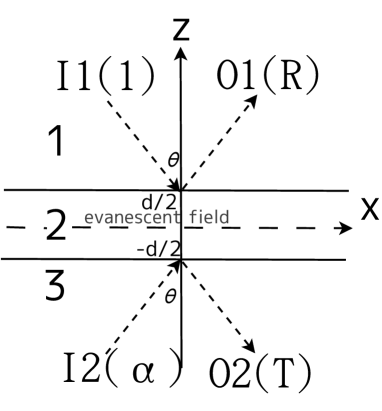
Figure 5: definition of parameters

With the boundary between region 1 and region 2 and in the large $d$ limit, which means to remove region 3, the injected light is reflected back to region 1 by the ’total reflection’, and there exists no light propagating into region 2 to $z$ direction. Instead, the evanescent light expressed by equation (71) is generated which decays in a short distance of order of wavelength exponentially according to distance from the boundary. Both (70) and (71) are solutions of the Maxwell’s equations, but usually (70) is not considered because the intensity of the electro-magnetic field becomes infinity at $z=-\infty$, contrary to locality that is common understanding of physics.

However, in the present model where the region 2 is not infinite but has a definite value of width (thickness), we have to be careful that equation (70) is finite intensity everywhere in region 2 and therefore we cannot neglect (70).

Different from the usual light propagation expressed by equations (10) and (11), the energy propagation in region 2 appears only in the cross term of (70) and (71) expressing the interaction of evanescent lights which decays exponentially to the directions of $+z$ and $-z$, respectively. This is supported with the fact that, in the large $d$ limit with fixed boundary between region 1 and region 2, where region 3 is removed, there occurs the total reflection and (71) becomes the only solution for region 2, and there exists no energy propagation to $-z$ direction in region 2.

We have calculated the electric field and magnetic field in region 2 from equations (70) and (71) as:

$${\bf E}^{2} =\begin{pmatrix}A^{(2,1)}_{TM}\sinh\varphi^{\prime}\\ A^{(2,1)}_{TE}\\ iA^{(2,1)}_{TM}\cosh\varphi^{\prime}\end{pmatrix}e^{i\left(\omega t-\frac{\cosh\varphi^{\prime}x+i\sinh\varphi^{\prime}z}{\lambdabar}\right)}$$

$$+\begin{pmatrix}A^{(2,2)}_{TM}\sinh\varphi^{\prime}\\ A^{(2,2)}_{TE}\\ -iA^{(2,2)}_{TM}\cosh\varphi^{\prime}\end{pmatrix}e^{i\left(\omega t-\frac{\cosh\varphi^{\prime}x-i\sinh\varphi^{\prime}z}{\lambdabar}\right)},$$ (72)

$${\bf B}^{2} =\frac{1}{\omega\lambdabar}\begin{pmatrix}-iA^{(2,1)}_{TE}\sinh\varphi^{\prime}\\ -iA^{(2,1)}_{TM}\\ A^{(2,1)}_{TE}\cosh\varphi^{\prime}\end{pmatrix}e^{i\left(\omega t-\frac{\cosh\varphi^{\prime}x+i\sinh\varphi^{\prime}z}{\lambdabar}\right)}$$

$$+\frac{1}{\omega\lambdabar}\begin{pmatrix}iA^{(2,2)}_{TE}\sinh\varphi^{\prime}\\ iA^{(2,2)}_{TM}\\ A^{(2,2)}_{TE}\cosh\varphi^{\prime}\end{pmatrix}e^{i\left(\omega t-\frac{\cosh\varphi^{\prime}x-i\sinh\varphi^{\prime}z}{\lambdabar}\right)}.$$ (73)

With derivation similar to that in section III, and using equations (18, 72, 22, 19, 73, 23), we have derived the independent boundary conditions at $z=\frac{d}{2}$ as:

$$\cos\theta(A^{1}_{TM}e^{i\frac{nd\cos\theta}{2\lambdabar}}+A^{R}_{TM}e^{-i\frac{nd\cos\theta}{2\lambdabar}})$$

$$=\sinh\varphi^{\prime}(A^{(2,1)}_{TM}e^{\frac{d\sinh\varphi^{\prime}}{2\lambdabar}}+A^{(2,2)}_{TM}e^{-\frac{d\sinh\varphi^{\prime}}{2\lambdabar}}),$$ (74)

$$n(A^{1}_{TM}e^{i\frac{nd\cos\theta}{2\lambdabar}}-A^{R}_{TM}e^{-i\frac{nd\cos\theta}{2\lambdabar}})$$

$$=i(A^{(2,1)}_{TM}e^{\frac{d\sinh\varphi^{\prime}}{2\lambdabar}}-A^{(2,2)}_{TM}e^{-\frac{d\sinh\varphi^{\prime}}{2\lambdabar}}),$$ (75)

$$A^{1}_{TE}e^{i\frac{nd\cos\theta}{2\lambdabar}}+A^{R}_{TE}e^{-i\frac{nd\cos\theta}{2\lambdabar}}$$

$$=A^{(2,1)}_{TE}e^{\frac{d\sinh\varphi^{\prime}}{2\lambdabar}}+A^{(2,2)}_{TE}e^{-\frac{d\sinh\varphi^{\prime}}{2\lambdabar}},$$ (76)

$$n\cos\theta(A^{1}_{TE}e^{i\frac{nd\cos\theta}{2\lambdabar}}-A^{R}_{TE}e^{-i\frac{nd\cos\theta}{2\lambdabar}})$$

$$=-i\sinh\varphi^{\prime}(A^{(2,1)}_{TE}e^{\frac{d\sinh\varphi^{\prime}}{2\lambdabar}}-A^{(2,2)}_{TE}e^{-\frac{d\sinh\varphi^{\prime}}{2\lambdabar}}).$$ (77)

and

$$\begin{pmatrix}A^{(2,1)}_{TM}e^{\frac{d\sinh\varphi^{\prime}}{2\lambdabar}}\\ A^{(2,2)}_{TM}e^{-\frac{d\sinh\varphi^{\prime}}{2\lambdabar}}\end{pmatrix}$$

$$=\!\!\begin{pmatrix}\frac{\cos\!\theta\!+\!in\!\sinh\!\varphi^{\prime}}{2\sinh\varphi^{\prime}}&\frac{\cos\!\theta\!-\!in\!\sinh\!\varphi^{\prime}}{2\sinh\varphi^{\prime}}\\ \frac{\cos\!\theta\!-\!in\!\sinh\!\varphi^{\prime}}{2\sinh\varphi^{\prime}}&\frac{\cos\!\theta\!+\!in\!\sinh\!\varphi^{\prime}}{2\sinh\varphi^{\prime}}\end{pmatrix}\!\!\begin{pmatrix}A^{3}_{TM}e^{i\frac{d\cos\theta}{2\lambdabar}}\\ A^{T}_{TM}e^{-i\frac{d\cos\theta}{2\lambdabar}}\end{pmatrix},$$ (78)

$$\begin{pmatrix}A^{(2,1)}_{TE}e^{\frac{d\omega\sinh\varphi^{\prime}}{2c_{2}}}\\ A^{(2,2)}_{TE}e^{-\frac{d\omega\sinh\varphi^{\prime}}{2c_{2}}}\end{pmatrix}$$

$$=\!\!\begin{pmatrix}\!\!\frac{n\cos\!\theta\!+\!i\sinh\!\varphi^{\prime}}{i\sinh\varphi^{\prime}}&\!\!-\frac{n\cos\!\theta\!-\!i\sinh\!\varphi^{\prime}}{i\sinh\varphi^{\prime}}\\ \!\!-\frac{n\cos\!\theta\!-\!i\sinh\!\varphi^{\prime}}{i\sinh\varphi^{\prime}}&\!\!\frac{n\cos\!\theta\!+\!i\sinh\!\varphi^{\prime}}{i\sinh\varphi^{\prime}}\end{pmatrix}\!\!\begin{pmatrix}A^{3}_{TE}e^{i\frac{nd\cos\!\theta}{2\lambdabar}}\\ A^{T}_{TE}e^{-i\frac{nd\cos\!\theta}{2\lambdabar}}\end{pmatrix}.$$ (79)

We have also derived those at $z=-\frac{d}{2}$ as:

$$\sinh\varphi^{\prime}(A^{(2,1)}_{TM}e^{-\frac{d\sinh\varphi^{\prime}}{2\lambdabar}}+A^{(2,2)}_{TM}e^{\frac{d\sinh\varphi^{\prime}}{2\lambdabar}})$$

$$=\cos\theta(A^{3}_{TM}e^{i\frac{nd\cos\theta}{2\lambdabar}}+A^{T}_{TM}e^{-i\frac{nd\cos\theta}{2\lambdabar}}),$$ (80)

$$i(A^{(2,1)}_{TM}e^{-\frac{d\sinh\varphi^{\prime}}{2\lambdabar}}-A^{(2,2)}_{TM}e^{\frac{d\sinh\varphi^{\prime}}{2\lambdabar}})$$

$$=-n(A^{3}_{TM}e^{i\frac{nd\cos\theta}{2\lambdabar}}-A^{T}_{TM}e^{-i\frac{nd\cos\theta}{2\lambdabar}}),$$ (81)

$$A^{(2,1)}_{TE}e^{-\frac{d\sinh\varphi^{\prime}}{2\lambdabar}}+A^{(2,2)}_{TE}e^{\frac{d\sinh\varphi^{\prime}}{2\lambdabar}}$$

$$=A^{3}_{TE}e^{i\frac{nd\cos\theta}{2\lambdabar}}+A^{T}_{TE}e^{-i\frac{nd\cos\theta}{2\lambdabar}},$$ (82)

$$-i\sinh\varphi^{\prime}(A^{(2,1)}_{TE}e^{-\frac{d\cos\theta}{2\lambdabar}}-A^{(2,2)}_{TE}e^{\frac{d\cos\theta}{2\lambdabar}})$$

$$=n\cos\theta(A^{3}_{TE}e^{i\frac{nd\cos\theta}{2\lambdabar}}-A^{T}_{TE}e^{-i\frac{nd\cos\theta}{2\lambdabar}}),$$ (83)

and

$$\begin{pmatrix}A^{(2,1)}_{TM}e^{-\frac{d\sinh\varphi^{\prime}}{2\lambdabar}}\\ A^{(2,2)}_{TM}e^{\frac{d\sinh\varphi^{\prime}}{2\lambdabar}}\end{pmatrix}$$

$$=\!\!\begin{pmatrix}\frac{\cos\!\theta\!+\!in\sinh\!\varphi^{\prime}}{2\sinh\varphi^{\prime}}&\!\!\frac{\cos\!\theta\!-\!in\sinh\!\varphi^{\prime}}{2\sinh\varphi^{\prime}}\\ \frac{\cos\!\theta\!-\!in\sinh\!\varphi^{\prime}}{2\sinh\varphi^{\prime}}&\!\!\frac{\cos\!\theta\!+\!in\sinh\!\varphi^{\prime}}{2\sinh\varphi^{\prime}}\end{pmatrix}\!\!\begin{pmatrix}\!\!A^{3}_{TM}e^{i\frac{nd\!\cos\!\theta}{2\lambdabar}}\\ \!\!A^{T}_{TM}e^{-i\frac{nd\!\cos\!\theta}{2\lambdabar}}\end{pmatrix},$$ (84)

$$\begin{pmatrix}A^{(2,1)}_{TE}e^{-\frac{d\sinh\varphi^{\prime}}{2\lambdabar}}\\ A^{(2,2)}_{TE}e^{\frac{d\sinh\varphi^{\prime}}{2\lambdabar}}\end{pmatrix}$$

$$=\!\!\begin{pmatrix}\frac{n\!\cos\!\theta\!+\!i\sinh\!\varphi^{\prime}}{i2\sinh\varphi^{\prime}}&\!\!-\frac{n\!\cos\!\theta\!-\!i\sinh\!\varphi^{\prime}}{i2\sinh\varphi^{\prime}}\\ -\frac{n\!\cos\!\theta\!-\!i\sinh\!\varphi^{\prime}}{i2\sinh\varphi^{\prime}}&\!\!\frac{n\!\cos\!\theta\!+\!i\sinh\!\varphi^{\prime}}{i2\sinh\varphi^{\prime}}\end{pmatrix}\!\!\begin{pmatrix}A^{3}_{TE}e^{i\frac{nd\cos\theta}{2\lambdabar}}\\ A^{T}_{TE}e^{-i\frac{nd\cos\theta}{2\lambdabar}}\end{pmatrix}.$$ (85)

From equations (78), (79), (84), (85), we have calculated the Poynting’s vectors as:

$$A^{R}_{TM} =\frac{\begin{bmatrix}-i(\!\cos^{2}\!\theta\!\!+\!\!n^{2}\!\sinh^{2}\!\varphi^{\prime}\!)\sinh(\!\frac{d\sinh\varphi^{\prime}}{\lambdabar}\!)A^{1}_{TM}\\ +2n\cos\theta\sinh\varphi^{\prime}A^{3}_{TM}\end{bmatrix}}{\begin{bmatrix}2n\cos\theta\sinh\varphi^{\prime}\cosh(\frac{d\sin\varphi^{\prime}}{\lambdabar})\\ +i(\cos^{2}\theta-n^{2}\sinh^{2}\varphi^{\prime})\sinh(\frac{d\sin\varphi^{\prime}}{\lambdabar})\end{bmatrix}}e^{in\frac{d\cos\theta}{\lambdabar}},$$ (86)

$$A^{R}_{TE} =\frac{\begin{bmatrix}i(n^{2}\!\!\cos^{2}\!\theta\!\!+\!\!\sinh^{2}\!\!\varphi^{\prime})\sinh(\frac{d\sinh\varphi^{\prime}}{\lambdabar})A^{1}_{TE}\\ +2n\cos\theta\sinh\varphi^{\prime}A^{3}_{TE}\end{bmatrix}}{\begin{bmatrix}2n\cos\theta\sinh\varphi^{\prime}\cosh(\frac{d\sin\varphi^{\prime}}{\lambdabar})\\ +i(n^{2}\cos^{2}\theta-\sinh^{2}\varphi^{\prime})\sinh(\frac{d\sin\varphi^{\prime}}{\lambdabar})\end{bmatrix}}e^{in\frac{d\cos\theta}{\lambdabar}},$$ (87)

and

$$A^{T}_{TM} =\frac{\begin{bmatrix}2n\cos\theta\sinh\varphi^{\prime}A^{1}_{TM}\\ -i(\cos^{2}\!\theta\!\!+\!\!n^{2}\!\sinh^{2}\!\!\varphi^{\prime}\!)\sinh(\!\frac{d\sinh\varphi^{\prime}}{\lambdabar}\!)A^{3}_{TM}\end{bmatrix}}{\begin{bmatrix}2n\cos\theta\sinh\varphi^{\prime}\cosh(\frac{d\sinh\varphi^{\prime}}{\lambdabar})\\ +i(\cos^{2}\theta-n^{2}\sinh^{2}\varphi^{\prime})\sinh(\frac{d\sinh\varphi^{\prime}}{\lambdabar})\end{bmatrix}}e^{in\frac{d\cos\theta}{\lambdabar}},$$ (88)

$$A^{T}_{TE} =\frac{\begin{bmatrix}2n\cos\theta\sinh\varphi^{\prime}A^{1}_{TE}\\ +i(n^{2}\!\!\cos^{2}\!\theta\!\!+\!\!\sinh^{2}\!\!\varphi^{\prime}\!)\sinh(\!\frac{d\sinh\varphi^{\prime}}{\lambdabar}\!\!)A^{3}_{TE}\end{bmatrix}}{\begin{bmatrix}2n\cos\theta\sinh\varphi^{\prime}\cosh(\frac{d\sin\varphi^{\prime}}{\lambdabar})\\ +i(n^{2}\cos^{2}\theta-\sinh^{2}\varphi^{\prime})\sinh(\frac{d\sin\varphi^{\prime}}{\lambdabar})\end{bmatrix}}e^{in\frac{d\cos\theta}{\lambdabar}}.$$ (89)

We have calculated the intensity ratios by taking the long time average as in section III:

$$\overline{R}_{TM} =\frac{\begin{bmatrix}(\cos^{2}\!\theta\!+\!n^{2}\!\sinh^{2}\!\varphi^{\prime})^{2}\sinh^{2}(\frac{d\omega\sinh\varphi^{\prime}}{c_{2}})\\ \!+\!4\alpha n^{2}\cos^{2}\!\theta\sinh^{2}\varphi^{\prime}\\ -4\sqrt{\alpha}n\sin\!\eta\cos\!\theta\sinh\!\varphi^{\prime}\\ \times\!(\cos^{2}\!\theta\!+\!n^{2}\!\sinh^{2}\!\varphi^{\prime})\!\sinh(\frac{d\sinh\varphi^{\prime}}{\lambdabar})\end{bmatrix}}{\begin{bmatrix}(\cos^{2}\!\theta\!+\!n^{2}\!\sinh^{2}\!\varphi^{\prime})^{2}\!\sinh^{2}(\frac{d\sinh\varphi^{\prime}}{\lambdabar})\\ +\!4n^{2}\cos^{2}\theta\sinh^{2}\varphi^{\prime}\end{bmatrix}},$$ (90)

$$\overline{R}_{TE} =\frac{\begin{bmatrix}(\sinh^{2}\!\varphi^{\prime}\!+\!n^{2}\!\cos^{2}\!\theta)^{2}\!\sinh^{2}(\frac{d\sinh\varphi^{\prime}}{\lambdabar})\\ +\!4\alpha n\sinh\!\varphi^{\prime}\cos\!\theta\\ +4\!\sin\!\eta\sqrt{\alpha}n\sinh\!\varphi^{\prime}\cos\!\theta\\ \times\!(\sinh^{2}\!\varphi^{\prime}\!+\!n^{2}\!\cos^{2}\!\theta)^{2}\!\sinh(\frac{d\sinh\varphi^{\prime}}{\lambdabar})\end{bmatrix}}{\begin{bmatrix}(\sinh^{2}\!\varphi^{\prime}\!+\!n^{2}\!\cos\!\theta)^{2}\!\sinh^{2}(\frac{d\sinh\!\varphi^{\prime}}{\lambdabar})\\ +4n^{2}\cos^{2}\!\theta\sinh^{2}\!\varphi^{\prime}\end{bmatrix}}.$$ (91)

Using Snell’s equation (64)and the definition of $\kappa$ expressed in equation (65), we have led the relations among $\kappa,\theta,n$, and $\varphi^{\prime}$ expressed as:

$$\frac{\sinh\varphi^{\prime}}{\cos\theta}=\sqrt{(n^{2}-1)\kappa-1},$$ (92)

$$\sinh\varphi^{\prime}=\sqrt{\frac{(n^{2}-1)\kappa-1}{\kappa+1}},$$ (93)

Using the relations (92) and (93), we have finally derived $\overline{R}_{TM}$ and $\overline{R}_{TE}$ as functions of $d,\lambdabar,\alpha,n$, and $\kappa$ as:

$$\overline{R}_{TM} =\frac{\begin{bmatrix}(n^{2}\!-1)^{2}(n^{2}\kappa\!-\!1)^{2}\!\sinh^{2}\bigl{(}\!\frac{d}{\lambdabar}\sqrt{\!\frac{(n^{2}\!-\!1)\kappa\!-\!1}{\kappa+1}}\bigr{)}\\ +\!4\alpha n^{2}[(n^{2}\!-\!1)\kappa\!-\!1]\\ -4\sqrt{\alpha}\sin\!\eta n\sqrt{(n^{2}\!-\!1)\kappa\!-\!1}\\ \times\!(n^{2}\!-\!1)(n^{2}\kappa\!-\!1)\!\sinh\bigl{(}\!\frac{d}{\lambdabar}\sqrt{\!\frac{(n^{2}\!-\!1)\kappa\!-\!1}{\kappa+1}}\bigr{)}\end{bmatrix}}{\begin{bmatrix}(n^{2}\!-\!1)^{2}\!(n^{2}\kappa\!-\!1)^{2}\!\sinh^{2}\bigl{(}\!\!\frac{d}{\lambdabar}\!\sqrt{\!\frac{(n^{2}\!-\!1)\kappa\!-\!1}{\kappa+1}}\bigr{)}\\ +4n^{2}[(n^{2}-1)\kappa-1]\end{bmatrix}},$$ (94)

$$\overline{R}_{TE} =\frac{\begin{bmatrix}(n^{2}\!-\!1)^{2}(\kappa\!+\!1)^{2}\sinh^{2}\bigl{(}\!\frac{d}{\lambdabar}\!\!\sqrt{\!\frac{(n^{2}\!-\!1)\kappa\!-\!1}{\kappa+1}}\!\bigr{)}\\ +4\alpha n^{2}[(n^{2}\!-\!1)\kappa\!-\!1]\\ +4n^{2}[(n^{2}-1)\kappa-1]\\ +4\sqrt{\alpha}\sin\!\eta n\sqrt{(n^{2}\!-\!1)\kappa\!-\!1}\\ \times\!(n^{2}\!-\!1)(\kappa\!+\!1)\!\sinh\bigl{(}\!\frac{d}{\lambdabar}\!\sqrt{\frac{(n^{2}\!-\!1)\kappa\!-\!1}{\kappa+1}}\bigr{)}\end{bmatrix}}{\begin{bmatrix}(n^{2}\!-\!1)^{2}(\kappa\!+\!1)^{2}\sinh^{2}\bigl{(}\frac{d}{\lambdabar}\!\!\sqrt{\frac{(n^{2}-1)\kappa-1}{\kappa+1}}\bigr{)}\\ +\!4n^{2}[(n^{2}-1)\kappa-1]\end{bmatrix}}.$$ (95)

V Conditions for $\overline{R}=0$

Summing up results in sections III and IV, we have attained the following equations:

$$\overline{R}_{TM} =\frac{\begin{bmatrix}(n^{2}\!-1)^{2}(n^{2}\kappa\!-\!1)^{2}\!S_{d}^{2}(\kappa)\\ +\!4\alpha n^{2}|(n^{2}\!-\!1)\kappa\!-\!1|\\ -4\sqrt{\alpha}\sin\!\eta n\sqrt{|(n^{2}\!-\!1)\kappa\!-\!1|}\\ \times\!(n^{2}\!-\!1)(n^{2}\kappa\!-\!1)\!S_{d}(\kappa)\end{bmatrix}}{\begin{bmatrix}(n^{2}\!-\!1)^{2}\!(n^{2}\kappa\!-\!1)^{2}\!S_{d}^{2}(\kappa)\\ +4n^{2}|(n^{2}-1)\kappa-1|\end{bmatrix}},$$ (96)

$$\overline{R}_{TE} =\frac{\begin{bmatrix}(n^{2}\!-\!1)^{2}(\kappa\!+\!1)^{2}S_{d}^{2}(\kappa)\\ +4\alpha n^{2}|(n^{2}\!-\!1)\kappa\!-\!1|\\ +4\sqrt{\alpha}\sin\!\eta n\sqrt{|(n^{2}\!-\!1)\kappa\!-\!1|}\\ \times\!(n^{2}\!-\!1)(\kappa\!+\!1)\!S_{d}(\kappa)\end{bmatrix}}{\begin{bmatrix}(n^{2}\!-\!1)^{2}(\kappa\!+\!1)^{2}S_{d}^{2}(\kappa)\\ +\!4n^{2}|(n^{2}-1)\kappa-1|\end{bmatrix}},$$ (97)

where

$$S_{d}(\kappa):=\left\{\begin{matrix}\sin\bigl{(}\!\frac{d}{\lambdabar}\!\sqrt{\!\frac{1-(n^{2}\!-\!1)\kappa}{1+\kappa}}\bigr{)},&\text{if }0\leq\kappa\leq\frac{1}{n^{2}-1},\\ \sinh\bigl{(}\!\frac{d}{\lambdabar}\!\sqrt{\!\frac{(n^{2}\!-\!1)\kappa\!-\!1}{\kappa+1}}\bigr{)},&\text{if }\frac{1}{n^{2}-1}\leq\kappa\end{matrix}\right..$$ (98)

At $\eta=\frac{\pi}{2}$ for TM mode and at $\eta=-\frac{\pi}{2}$ for TE mode, we have derived equations (96) and (97) respectively:

$$\overline{R}_{TM} =\frac{\begin{bmatrix}\left[(n^{2}\!-1)(n^{2}\kappa\!-\!1)\!S_{d}(\kappa)\right.\\ \left.-\!2\sqrt{\alpha}n\sqrt{|(n^{2}\!-\!1)\kappa\!-\!1|}\right]^{2}\end{bmatrix}}{\begin{bmatrix}(n^{2}\!-\!1)^{2}\!(n^{2}\kappa\!-\!1)^{2}\!S_{d}^{2}(\kappa)\\ +4n^{2}|(n^{2}-1)\kappa-1|\end{bmatrix}},$$ (99)

$$\overline{R}_{TE} =\frac{\begin{bmatrix}\left[(n^{2}\!-\!1)(\kappa\!+\!1)S_{d}(\kappa)\right.\\ \left.-2\sqrt{\alpha}n\sqrt{|(n^{2}\!-\!1)\kappa\!-\!1|}\right]^{2}\end{bmatrix}}{\begin{bmatrix}(n^{2}\!-\!1)^{2}(\kappa\!+\!1)^{2}S_{d}^{2}(\kappa)\\ +\!4n^{2}|(n^{2}-1)\kappa-1|\end{bmatrix}}.$$ (100)

Because each of the numerators of (99) and (100) is perfect square of a difference, we can realize $\overline{R}_{TM}=0$ or $\overline{R}_{TE}=0$ by selecting appropriate values for a set of free parameters $(\kappa,\alpha,n)$. For TM mode, those parameters should satisfy:

$$(n^{2}-1)(n^{2}\kappa-1)S_{d}(\kappa)=2\sqrt{\alpha}n\sqrt{|(n^{2}-1)\kappa-1|},$$ (101)

and for TE mode:

$$(n^{2}-1)(\kappa+1)S_{d}(\kappa)=2\sqrt{\alpha}n\sqrt{|(n^{2}-1)\kappa-1|}.$$ (102)

Rewriting (101) and (102):

$$\alpha =\frac{(n^{2}-1)^{2}(n^{2}\kappa-1)^{2}S_{d}^{2}(\kappa)}{4n^{2}|(n^{2}-1)\kappa-1|}, TM\text{ mode},$$ (103)

$$\alpha =\frac{(n^{2}-1)^{2}(\kappa+1)^{2}S_{d}^{2}(\kappa)}{4n^{2}|(n^{2}-1)\kappa-1|}, TE\text{ mode}.$$ (104)

Equations (103) and (104) are shown in Figs.6 and 7, respectively, for $n=1.5$.

\psfrag{kappa}{$\kappa$}\psfrag{alpha}{$\alpha$}\psfrag{d/l=pi/2}[Br][Br]{$d/\lambdabar=\frac{\pi}{2}$}\psfrag{d/l=pi}[Br][Br]{$d/\lambdabar=\pi$}\psfrag{d/l=4}[Br][Br]{$d/\lambdabar=4$}\psfrag{1/n^2}{$\frac{1}{n^{2}}$}\psfrag{1/(n^2-1)}{$\frac{1}{n^{2}-1}$}\includegraphics[width=199.16928pt]{3over2TM.eps}

Figure 6: $\kappa-\alpha$ relation for $TM$ mode with $n=1.5$

\psfrag{kappa}{$\kappa$}\psfrag{alpha}{$\alpha$}\psfrag{d/l=pi/2}[Br][Br]{$d/\lambdabar=\frac{\pi}{2}$}\psfrag{d/l=pi}[Br][Br]{$d/\lambdabar=\pi$}\psfrag{d/l=4}[Br][Br]{$d/\lambdabar=4$}\psfrag{1/(n^2-1)}{$\frac{1}{n^{2}-1}$}\includegraphics[width=199.16928pt]{3over2TE.eps}

Figure 7: $\kappa-\alpha$ relation for $TE$ mode with $n=1.5$

Namely, when $\alpha$ is on either curve of Fig.6 or Fig.7, $\overline{R}_{TM}$ or $\overline{R}_{TE}$ can be switched to $0$ and a finite value depending on $\eta$ as:

$$\overline{R}_{TM} =\left\{\begin{array}[]{cl}0,&\text{at }\eta=\frac{\pi}{2},\\ \frac{4\alpha}{\alpha+1},&\text{at }\eta=-\frac{\pi}{2}\end{array}\right.,$$ (107)

$$\overline{R}_{TE} =\left\{\begin{array}[]{cl}0,&\text{at }\eta=-\frac{\pi}{2},\\ \frac{4\alpha}{\alpha+1},&\text{at }\eta=\frac{\pi}{2}\end{array}\right..$$ (110)

\psfrag{ALPHA}{$\frac{4\alpha}{\alpha+1}$}\psfrag{alpha}{$\alpha$}\includegraphics[width=199.16928pt]{Ron.eps}

Figure 8: $\overline{R}$ at $\eta=\eta_{0}+\pi$

The finite value of $\overline{R}$ above is shown in Fig.8 as a function of $\alpha$. Equations (107) and (110) tell that when this device is coupled with a Mach-Zehnder interferometer of Fig.1 and composed as an optical switch as Fig.1 using some kind of phase controller in one of transmission lines of the interferometer, the intensity of the output light at ’on’ does not explicitly depend on incision angle $\theta$ nor width of vacuum layer $d$.

Finally, we will discuss on inverse functions $\kappa=\kappa(\alpha)$ of equations (103) and (104). For equations (107) and (110), it seems more realistic to decide incision angle $\theta$ corresponding to $\overline{R}$ after deciding the intensity ratio $\alpha$ of the light intensity of I2 to that of I1.

For TM mode, equation (103) shows that $\alpha$ is a monotonic increasing function of $\kappa\in[\frac{1}{n^{2}},\infty)$ with $\alpha(\frac{1}{n^{2}})=0$ and $\alpha\rightarrow\infty$ in large $\kappa$ limit, so that for any $\alpha\geq 0$, there uniquely exists $\kappa\in[\frac{1}{n^{2}},\infty)$ which satisfy equation (103).

On the other hand, for TE mode, as shown by Fig.7, there exists some range of $\alpha$ value which cannot be reached for any $\kappa$ value. Actually, equation (104) becomes around $\kappa=0$,

$$\alpha =\frac{(n^{2}-1)^{2}}{4n^{2}}\sin^{2}\bigl{(}\frac{d}{\lambdabar}\bigr{)}$$

$$+\!\!\frac{(n^{2}\!\!-\!\!1)^{2}\!(n^{2}\!\!+\!\!1)^{2}}{8n^{2}}\!\sin\bigl{(}\!\frac{2d}{\lambdabar}\!\bigr{)}\!\bigl{\{}\!\tan\bigl{(}\!\frac{d}{\lambdabar}\!\bigr{)}\!-\!\frac{n^{2}}{n^{2}\!+\!1}\frac{d}{\lambdabar}\!\bigr{\}}\kappa$$

$$+O(\kappa^{2}).$$ (111)

The coefficient of the first order of $\kappa$ in equation (111) is positive for a region $0\leq\frac{d}{\lambdabar}<\pi$, and within this region, $\alpha$ is a monotonic increasing function of $\kappa$ around $\kappa=0$. Therefore, in the region $0\leq\frac{d}{\lambdabar}<\pi$, the $\alpha$ takes the minimum value $\frac{(n^{2}-1)^{2}}{4n^{2}}\sin^{2}\bigl{(}\frac{d}{\lambdabar}\bigr{)}$ at $\kappa=0$. For the region $\pi\leq\frac{d}{\lambdabar}$, since $\alpha=0$ at $\kappa=\frac{d-\pi\lambdabar}{dn^{2}+\pi\lambdabar-d}$, there exists at least one $\kappa\geq\frac{d-\pi\lambdabar}{dn^{2}+\pi\lambdabar-d}$ for any $\alpha\geq 0$.

Based on those discussion results, we have attained the following statements for $\alpha$ value for $\overline{R}_{TE}=0$ in TE mode:

• for $0\leq\frac{d}{\lambdabar}<\pi$:
  There exists a $\kappa$ for $\overline{R}_{TE}=0$ for any non-negative value of $\alpha$ larger than $\frac{(n^{2}-1)^{2}}{4n^{2}}\sin^{2}\bigl{(}\frac{d}{\lambdabar}\bigr{)}$, and

• for $\pi\leq\frac{d}{\lambdabar}$:
  there exists $\kappa$ for $\overline{R}_{TE}=0$ for any non-negative value of $\alpha$.

VI Conclusion

We have taken as the study model an infinite dielectric region with refractive index $n$ divided by an two dimensionally infinite vacuum layer between $z=\frac{d}{2}$ and $z=-\frac{d}{2}$. Two input lights are injected from the upper region 1 ($z>\frac{d}{2}$) and the lower region ($z<-\frac{d}{2}$) with intensity of 1 and $\alpha$, respectively, and with the same injection angle $\theta$. We have solved the intensity of output lights into region 1 and 3 directly from the Maxwell’s equations. As the results, we have found that one of two output lights can be made zero by appropriately selecting set of values of $\alpha$, phase difference of the two input lights $\eta$, $d$ and $\theta$. Namely,

1. There exists a set of parameters $(\alpha_{0},\theta_{0},d_{0},\eta_{0})$ that makes one of output light zero ($\overline{R}=0$). And for these set of values and replacing $\eta_{0}$ to $\eta_{0}+\pi$,

   $$\overline{R}=\frac{4\alpha}{\alpha+1}.$$

   Here $\eta_{0}$ is $\frac{\pi}{2}$ for TM mode and $-\frac{\pi}{2}$ for TE mode,

2. When a TM mode light is used as the input light, for any set of $(\theta,d)$, a value of $\alpha$ can be obtained by equation (103) which makes $\overline{R}=0$ at $\eta=\frac{\pi}{2}$. Particularly for $\theta$ larger than the critical angle and evanescent light exist in region 2 (vacuum region between upper and lower dielectric region), $\alpha$ for $\overline{R}=0$ satisfies $\alpha\geq\frac{(n^{2}-1)^{2}}{4n^{4}}(\frac{d}{\lambdabar})^{2}$, and

3. When a TE mode light is used as the input light, for any set of $(\theta,d)$, a value of $\alpha$ can be obtained by equation (104) which makes $\overline{R}=0$ at $\eta=-\frac{\pi}{2}$. Particularly for $\theta$ larger than the critical angle and evanescent light exist in region 2, $\alpha$ for $\overline{R}=0$ satisfies $\alpha\geq\frac{n^{2}-1}{4}(\frac{d}{\lambdabar})^{2}$.

The above results 1-3 suggests a possibility that, using a Mach-Zehnder interferometer with controlling phase difference between two transmission lines to $\frac{\pi}{2}$ or $-\frac{\pi}{2}$, we can control the output light on and off. One point is that the output light is perfectly eliminated at switched ’off’ without depending on $\alpha$. This tells that the new switch proposed here is better than the usual Mach-Zehnder interferometer because in a Mach-Zehnder interferometer, a perfect branching of input light of 50 : 50 is necessary to get the output zero at ’off’. More notable point better than a Mach-Zehnder interferometer is that, the output light is controlled to on and off with a light much weaker than the output light at ’on’. In a case of $\alpha=0.10$ for example, the output light intensity at ’on’ is $\frac{4\alpha}{\alpha+1}=0.36$. In this case, the output light is controlled by a control light with intensity of $\frac{1}{3.6}$ of the output light. From engineering point of view, this means that a control light can be divided to several optical switches which is one of critically important features for the switch to be applied in logic circuits.

Since a real optical device has a finite size of several to ten times larger than the light wavelength whereas an infinite model is studied in this paper, effects of finite size such as the effect of the higher modes must be investigated in future. Furthermore, effect of real boundary plane being not perfectly flat and not perfectly parallel shall also be investigated.

References

(1)John David Jackson: Classical Electrodynamics,
John Willey & Sons, Inc. (1974)
(2)Edward M. Purcell: ELECTRICITY AND MAGNETISM,
Berkeley Physics Course, McGraw-Hill, Inc. (1985)