B. Aubert
M. Bona
Y. Karyotakis
J. P. Lees
V. Poireau
E. Prencipe
X. Prudent
V. Tisserand
Laboratoire de Physique des Particules, IN2P3/CNRS et Université de Savoie, F-74941 Annecy-Le-Vieux, France
J. Garra Tico
E. Grauges
Universitat de Barcelona, Facultat de Fisica, Departament ECM, E-08028 Barcelona, Spain
L. LopezabA. PalanoabM. PappagalloabINFN Sezione di Baria; Dipartmento di Fisica, Università di Barib, I-70126 Bari, Italy
G. Eigen
B. Stugu
L. Sun
University of Bergen, Institute of Physics, N-5007 Bergen, Norway
G. S. Abrams
M. Battaglia
D. N. Brown
R. G. Jacobsen
L. T. Kerth
Yu. G. Kolomensky
G. Lynch
I. L. Osipenkov
M. T. Ronan
K. Tackmann
T. Tanabe
Lawrence Berkeley National Laboratory and University of California, Berkeley, California 94720, USA
C. M. Hawkes
N. Soni
A. T. Watson
University of Birmingham, Birmingham, B15 2TT, United Kingdom
H. Koch
T. Schroeder
Ruhr Universität Bochum, Institut für Experimentalphysik 1, D-44780 Bochum, Germany
D. J. Asgeirsson
B. G. Fulsom
C. Hearty
T. S. Mattison
J. A. McKenna
University of British Columbia, Vancouver, British Columbia, Canada V6T 1Z1
M. Barrett
A. Khan
Brunel University, Uxbridge, Middlesex UB8 3PH, United Kingdom
V. E. Blinov
A. D. Bukin
A. R. Buzykaev
V. P. Druzhinin
V. B. Golubev
A. P. Onuchin
S. I. Serednyakov
Yu. I. Skovpen
E. P. Solodov
K. Yu. Todyshev
Budker Institute of Nuclear Physics, Novosibirsk 630090, Russia
M. Bondioli
S. Curry
I. Eschrich
D. Kirkby
A. J. Lankford
P. Lund
M. Mandelkern
E. C. Martin
D. P. Stoker
University of California at Irvine, Irvine, California 92697, USA
S. Abachi
C. Buchanan
University of California at Los Angeles, Los Angeles, California 90024, USA
H. Atmacan
J. W. Gary
F. Liu
O. Long
G. M. Vitug
Z. Yasin
L. Zhang
University of California at Riverside, Riverside, California 92521, USA
V. Sharma
University of California at San Diego, La Jolla, California 92093, USA
C. Campagnari
T. M. Hong
D. Kovalskyi
M. A. Mazur
J. D. Richman
University of California at Santa Barbara, Santa Barbara, California 93106, USA
T. W. Beck
A. M. Eisner
C. J. Flacco
C. A. Heusch
J. Kroseberg
W. S. Lockman
A. J. Martinez
T. Schalk
B. A. Schumm
A. Seiden
M. G. Wilson
L. O. Winstrom
University of California at Santa Cruz, Institute for Particle Physics, Santa Cruz, California 95064, USA
C. H. Cheng
D. A. Doll
B. Echenard
F. Fang
D. G. Hitlin
I. Narsky
T. Piatenko
F. C. Porter
California Institute of Technology, Pasadena, California 91125, USA
R. Andreassen
G. Mancinelli
B. T. Meadows
K. Mishra
M. D. Sokoloff
University of Cincinnati, Cincinnati, Ohio 45221, USA
P. C. Bloom
W. T. Ford
A. Gaz
J. F. Hirschauer
M. Nagel
U. Nauenberg
J. G. Smith
S. R. Wagner
University of Colorado, Boulder, Colorado 80309, USA
R. Ayad
Now at Temple University, Philadelphia, Pennsylvania 19122, USA
A. Soffer
Now at Tel Aviv University, Tel Aviv, 69978, Israel
W. H. Toki
R. J. Wilson
Colorado State University, Fort Collins, Colorado 80523, USA
E. Feltresi
A. Hauke
H. Jasper
M. Karbach
J. Merkel
A. Petzold
B. Spaan
K. Wacker
Technische Universität Dortmund, Fakultät Physik, D-44221 Dortmund, Germany
M. J. Kobel
R. Nogowski
K. R. Schubert
R. Schwierz
A. Volk
Technische Universität Dresden, Institut für Kern- und Teilchenphysik, D-01062 Dresden, Germany
D. Bernard
G. R. Bonneaud
E. Latour
M. Verderi
Laboratoire Leprince-Ringuet, CNRS/IN2P3, Ecole Polytechnique, F-91128 Palaiseau, France
P. J. Clark
S. Playfer
J. E. Watson
University of Edinburgh, Edinburgh EH9 3JZ, United Kingdom
M. AndreottiabD. BettoniaC. BozziaR. CalabreseabA. CecchiabG. CibinettoabP. FranchiniabE. LuppiabM. NegriniabA. PetrellaabL. PiemonteseaV. SantoroabINFN Sezione di Ferraraa; Dipartimento di Fisica, Università di Ferrarab, I-44100 Ferrara, Italy
R. Baldini-Ferroli
A. Calcaterra
R. de Sangro
G. Finocchiaro
S. Pacetti
P. Patteri
I. M. Peruzzi
Also with Università di Perugia, Dipartimento di Fisica, Perugia, Italy
M. Piccolo
M. Rama
A. Zallo
INFN Laboratori Nazionali di Frascati, I-00044 Frascati, Italy
A. BuzzoaR. ContriabM. Lo VetereabM. M. MacriaM. R. MongeabS. PassaggioaC. PatrignaniabE. RobuttiaA. SantroniabS. TosiabINFN Sezione di Genovaa; Dipartimento di Fisica, Università di Genovab, I-16146 Genova, Italy
K. S. Chaisanguanthum
M. Morii
Harvard University, Cambridge, Massachusetts 02138, USA
A. Adametz
J. Marks
S. Schenk
U. Uwer
Universität Heidelberg, Physikalisches Institut, Philosophenweg 12, D-69120 Heidelberg, Germany
V. Klose
H. M. Lacker
Humboldt-Universität zu Berlin, Institut für Physik, Newtonstr. 15, D-12489 Berlin, Germany
D. J. Bard
P. D. Dauncey
M. Tibbetts
Imperial College London, London, SW7 2AZ, United Kingdom
P. K. Behera
X. Chai
M. J. Charles
U. Mallik
University of Iowa, Iowa City, Iowa 52242, USA
J. Cochran
H. B. Crawley
L. Dong
W. T. Meyer
S. Prell
E. I. Rosenberg
A. E. Rubin
Iowa State University, Ames, Iowa 50011-3160, USA
Y. Y. Gao
A. V. Gritsan
Z. J. Guo
C. K. Lae
Johns Hopkins University, Baltimore, Maryland 21218, USA
N. Arnaud
J. Béquilleux
A. D’Orazio
M. Davier
J. Firmino da Costa
G. Grosdidier
F. Le Diberder
V. Lepeltier
A. M. Lutz
S. Pruvot
P. Roudeau
M. H. Schune
J. Serrano
V. Sordini
Also with Università di Roma La Sapienza, I-00185 Roma, Italy
A. Stocchi
G. Wormser
Laboratoire de l’Accélérateur Linéaire, IN2P3/CNRS et Université Paris-Sud 11, Centre Scientifique d’Orsay, B. P. 34, F-91898 Orsay Cedex, France
D. J. Lange
D. M. Wright
Lawrence Livermore National Laboratory, Livermore, California 94550, USA
I. Bingham
J. P. Burke
C. A. Chavez
J. R. Fry
E. Gabathuler
R. Gamet
D. E. Hutchcroft
D. J. Payne
C. Touramanis
University of Liverpool, Liverpool L69 7ZE, United Kingdom
A. J. Bevan
C. K. Clarke
F. Di Lodovico
R. Sacco
M. Sigamani
Queen Mary, University of London, London, E1 4NS, United Kingdom
G. Cowan
S. Paramesvaran
A. C. Wren
University of London, Royal Holloway and Bedford New College, Egham, Surrey TW20 0EX, United Kingdom
D. N. Brown
C. L. Davis
University of Louisville, Louisville, Kentucky 40292, USA
A. G. Denig
M. Fritsch
W. Gradl
Johannes Gutenberg-Universität Mainz, Institut für Kernphysik, D-55099 Mainz, Germany
K. E. Alwyn
D. Bailey
R. J. Barlow
G. Jackson
G. D. Lafferty
T. J. West
J. I. Yi
University of Manchester, Manchester M13 9PL, United Kingdom
J. Anderson
C. Chen
A. Jawahery
D. A. Roberts
G. Simi
J. M. Tuggle
University of Maryland, College Park, Maryland 20742, USA
C. Dallapiccola
X. Li
E. Salvati
S. Saremi
University of Massachusetts, Amherst, Massachusetts 01003, USA
R. Cowan
D. Dujmic
P. H. Fisher
S. W. Henderson
G. Sciolla
M. Spitznagel
F. Taylor
R. K. Yamamoto
M. Zhao
Massachusetts Institute of Technology, Laboratory for Nuclear Science, Cambridge, Massachusetts 02139, USA
P. M. Patel
S. H. Robertson
McGill University, Montréal, Québec, Canada H3A 2T8
A. LazzaroabV. LombardoaF. PalomboabINFN Sezione di Milanoa; Dipartimento di Fisica, Università di Milanob, I-20133 Milano, Italy
J. M. Bauer
L. Cremaldi
R. Godang
Now at University of South Alabama, Mobile, Alabama 36688, USA
R. Kroeger
D. J. Summers
H. W. Zhao
University of Mississippi, University, Mississippi 38677, USA
M. Simard
P. Taras
Université de Montréal, Physique des Particules, Montréal, Québec, Canada H3C 3J7
H. Nicholson
Mount Holyoke College, South Hadley, Massachusetts 01075, USA
G. De NardoabL. ListaaD. MonorchioabG. OnoratoabC. SciaccaabINFN Sezione di Napolia; Dipartimento di Scienze Fisiche, Università di Napoli Federico IIb, I-80126 Napoli, Italy
G. Raven
H. L. Snoek
NIKHEF, National Institute for Nuclear Physics and High Energy Physics, NL-1009 DB Amsterdam, The Netherlands
C. P. Jessop
K. J. Knoepfel
J. M. LoSecco
W. F. Wang
University of Notre Dame, Notre Dame, Indiana 46556, USA
L. A. Corwin
K. Honscheid
H. Kagan
R. Kass
J. P. Morris
A. M. Rahimi
J. J. Regensburger
S. J. Sekula
Q. K. Wong
Ohio State University, Columbus, Ohio 43210, USA
N. L. Blount
J. Brau
R. Frey
O. Igonkina
J. A. Kolb
M. Lu
R. Rahmat
N. B. Sinev
D. Strom
J. Strube
E. Torrence
University of Oregon, Eugene, Oregon 97403, USA
G. CastelliabN. GagliardiabM. MargoniabM. MorandinaM. PosoccoaM. RotondoaF. SimonettoabR. StroiliabC. VociabINFN Sezione di Padovaa; Dipartimento di Fisica, Università di Padovab, I-35131 Padova, Italy
P. del Amo Sanchez
E. Ben-Haim
H. Briand
G. Calderini
J. Chauveau
O. Hamon
Ph. Leruste
J. Ocariz
A. Perez
J. Prendki
S. Sitt
Laboratoire de Physique Nucléaire et de Hautes Energies, IN2P3/CNRS, Université Pierre et Marie Curie-Paris6, Université Denis Diderot-Paris7, F-75252 Paris, France
L. Gladney
University of Pennsylvania, Philadelphia, Pennsylvania 19104, USA
M. BiasiniabE. ManoniabINFN Sezione di Perugiaa; Dipartimento di Fisica, Università di Perugiab, I-06100 Perugia, Italy
C. AngeliniabG. BatignaniabS. BettariniabM. CarpinelliabAlso with Università di Sassari, Sassari, Italy
A. CervelliabF. FortiabM. A. GiorgiabA. LusianiacG. MarchioriabM. MorgantiabN. NeriabE. PaoloniabG. RizzoabJ. J. WalshaINFN Sezione di Pisaa; Dipartimento di Fisica, Università di Pisab; Scuola Normale Superiore di Pisac, I-56127 Pisa, Italy
D. Lopes Pegna
C. Lu
J. Olsen
A. J. S. Smith
A. V. Telnov
Princeton University, Princeton, New Jersey 08544, USA
F. AnulliaE. BaracchiniabG. CavotoaR. FacciniabF. FerrarottoaF. FerroniabM. GasperoabP. D. JacksonaL. Li GioiaM. A. MazzoniaS. MorgantiaG. PireddaaF. RengaabC. VoenaaINFN Sezione di Romaa; Dipartimento di Fisica, Università di Roma La Sapienzab, I-00185 Roma, Italy
M. Ebert
T. Hartmann
H. Schröder
R. Waldi
Universität Rostock, D-18051 Rostock, Germany
T. Adye
B. Franek
E. O. Olaiya
F. F. Wilson
Rutherford Appleton Laboratory, Chilton, Didcot, Oxon, OX11 0QX, United Kingdom
S. Emery
M. Escalier
L. Esteve
G. Hamel de Monchenault
W. Kozanecki
G. Vasseur
Ch. Yèche
M. Zito
CEA, Irfu, SPP, Centre de Saclay, F-91191 Gif-sur-Yvette, France
X. R. Chen
H. Liu
W. Park
M. V. Purohit
R. M. White
J. R. Wilson
University of South Carolina, Columbia, South Carolina 29208, USA
M. T. Allen
D. Aston
R. Bartoldus
J. F. Benitez
R. Cenci
J. P. Coleman
M. R. Convery
J. C. Dingfelder
J. Dorfan
G. P. Dubois-Felsmann
W. Dunwoodie
R. C. Field
A. M. Gabareen
M. T. Graham
P. Grenier
C. Hast
W. R. Innes
J. Kaminski
M. H. Kelsey
H. Kim
P. Kim
M. L. Kocian
D. W. G. S. Leith
S. Li
B. Lindquist
S. Luitz
V. Luth
H. L. Lynch
D. B. MacFarlane
H. Marsiske
R. Messner
D. R. Muller
H. Neal
S. Nelson
C. P. O’Grady
I. Ofte
M. Perl
B. N. Ratcliff
A. Roodman
A. A. Salnikov
R. H. Schindler
J. Schwiening
A. Snyder
D. Su
M. K. Sullivan
K. Suzuki
S. K. Swain
J. M. Thompson
J. Va’vra
A. P. Wagner
M. Weaver
C. A. West
W. J. Wisniewski
M. Wittgen
D. H. Wright
H. W. Wulsin
A. K. Yarritu
K. Yi
C. C. Young
V. Ziegler
Stanford Linear Accelerator Center, Stanford, California 94309, USA
P. R. Burchat
A. J. Edwards
T. S. Miyashita
Stanford University, Stanford, California 94305-4060, USA
S. Ahmed
M. S. Alam
J. A. Ernst
B. Pan
M. A. Saeed
S. B. Zain
State University of New York, Albany, New York 12222, USA
S. M. Spanier
B. J. Wogsland
University of Tennessee, Knoxville, Tennessee 37996, USA
R. Eckmann
J. L. Ritchie
A. M. Ruland
C. J. Schilling
R. F. Schwitters
University of Texas at Austin, Austin, Texas 78712, USA
B. W. Drummond
J. M. Izen
X. C. Lou
University of Texas at Dallas, Richardson, Texas 75083, USA
F. BianchiabD. GambaabM. PelliccioniabINFN Sezione di Torinoa; Dipartimento di Fisica Sperimentale, Università di Torinob, I-10125 Torino, Italy
M. BombenabL. BosisioabC. CartaroabG. Della RiccaabL. LanceriabL. VitaleabINFN Sezione di Triestea; Dipartimento di Fisica, Università di Triesteb, I-34127 Trieste, Italy
V. Azzolini
N. Lopez-March
F. Martinez-Vidal
D. A. Milanes
A. Oyanguren
IFIC, Universitat de Valencia-CSIC, E-46071 Valencia, Spain
J. Albert
Sw. Banerjee
B. Bhuyan
H. H. F. Choi
K. Hamano
R. Kowalewski
M. J. Lewczuk
I. M. Nugent
J. M. Roney
R. J. Sobie
University of Victoria, Victoria, British Columbia, Canada V8W 3P6
T. J. Gershon
P. F. Harrison
J. Ilic
T. E. Latham
G. B. Mohanty
Department of Physics, University of Warwick, Coventry CV4 7AL, United Kingdom
H. R. Band
X. Chen
S. Dasu
K. T. Flood
Y. Pan
R. Prepost
C. O. Vuosalo
S. L. Wu
University of Wisconsin, Madison, Wisconsin 53706, USA
Abstract
We report on a Dalitz plot analysis of decays, based on a sample of
about decays collected with the BABAR detector
at the PEP-II asymmetric-energy Factory at SLAC.
We find the total branching fraction of the three-body decay:
.
We observe the established and confirm the existence of in their decays to ,
where the and are the and P-wave states, respectively.
We measure the masses and widths of and to be:
,
,
and .
The stated errors reflect the statistical and systematic uncertainties,
and the uncertainty related to the assumed composition of signal events
and the theoretical model.
pacs:
13.25.Hw, 14.40.Lb, 14.40.Nd
I INTRODUCTION
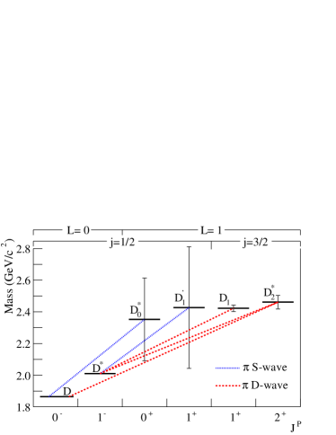
Orbitally excited states of the meson, denoted here as ,
where is the spin of the meson, provide a unique opportunity to test
the Heavy Quark Effective Theory (HQET) hqet1 ; hqet2 .
The simplest meson consists of a charm quark and a light anti-quark in
an orbital angular momentum (P-wave) state.
Four such states are expected with spin-parity
, , and ,
which are labeled here as , , and , respectively,
where is a quantum number corresponding to the sum of the light quark spin and the orbital
angular momentum .
The conservation of parity and angular momentum in strong interactions imposes constraints
on the strong decays of states to and .
The states are predicted to decay exclusively through an S-wave:
and .
The states are expected to decay through a D-wave:
and and .
These transitions are summarized in Fig. 1.
Because of the finite -quark mass, the two states
may be mixtures of the and states.
Thus the broad state may decay via a D-wave and
the narrow state may decay via an S-wave.
The states with , which decay through an
S-wave, are expected to be wide (hundreds of ),
while the states that decay through a D-wave are expected to
be narrow (tens of ) hqet2 ; falk ; falk2 .
Properties of the mesons PDG
are given in Table 1.
The narrow mesons have been previously observed and studied by a number of
experiments argus ; e691 ; cleo1 ; cleo2 ; e687 ; cleo3 ; belle-prd ; focus ; belle-d1todpp ; cdf ; belle-d0pp .
mesons have also been studied in semileptonic decays aleph ; cleo-semi ; D0 ; delphi ; babar-051101 ; belle-liventsev ; babar-0333 ; babar-0528 .
Precise knowledge of the properties of the mesons is important to reduce uncertainties in the measurements
of semileptonic decays, and thus the determination of the Cabibbo-Kobayashi-Maskawa CKM matrix elements and .
The Belle Collaboration has reported the first observation of the
broad and mesons in decay belle-prd .
The FOCUS Collaboration has found evidence for broad structures in final states focus with
mass and width in agreement with the found by Belle Collaboration.
However, the Particle Data Group PDG considers that the and quantum numbers of
the and states still need confirmation.
In this analysis, we fully reconstruct the decays conjugate
and measure their branching fraction.
We also perform an analysis of the Dalitz plot (DP) to measure the exclusive branching fractions of
and study the properties of the mesons.
The decay is expected to be dominated by the
intermediate states and , and has a possible
contribution from nonresonant (NR) decay.
The and states can not decay strongly
into because of parity and angular momentum conservation.
However, the (labeled as here) mass is close to the production
threshold and it may contribute as a virtual intermediate state.
The (labeled as here) produced in a virtual process may also contribute via
the decay .
Possible contributions from these virtual states are also studied in this analysis.
Figure 1: Mass spectrum for states.
The vertical bars show the widths.
Masses and widths are from Ref. PDG .
The dotted and dashed lines between the levels show the dominant pion transitions.
Although it is not indicated in the figure,
the two states may be mixtures of and , and
may decay via a D-wave and may decay via an S-wave.
The data used in this analysis were collected with the BABAR detector
at the PEP-II asymmetric-energy storage rings at SLAC between 1999 and
2006. The sample consists of 347.2 corresponding
to pairs () taken on the peak of the resonance.
Monte Carlo (MC) simulation is used to study the detector response, its acceptance, background,
and to validate the analysis.
We use GEANT4 geant4 to simulate resonant events
(generated by EvtGen evtgen ) and (where or ) continuum events
(generated by JETSET jetset ).
A detailed description of the BABAR detector is given in Ref. babarNim .
Charged particle trajectories are measured by a five-layer, double-sided
silicon vertex tracker (SVT) and a 40-layer drift chamber (DCH) immersed
in a 1.5 T magnetic field. Charged particle identification (PID) is achieved
by combining information from a ring-imaging Cherenkov device with
ionization energy loss () measurements in the DCH and SVT.
III EVENT SELECTION
Five charged particles are selected to reconstruct decays of with .
The charged particle candidates are required to have
transverse momenta above and at least twelve hits in the DCH.
A candidate must be identified as a kaon using a likelihood-based particle identification
algorithm (with an average efficiency of 85% and an average misidentification probability of 3%).
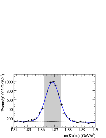
Any combination of candidates with a common vertex and an invariant
mass between 1.8625 and 1.8745 is accepted as a candidate.
We fit the invariant mass distribution of the candidates
with a function that includes a Gaussian component for the
signal and a linear term for the background.
The signal parameters (mean and width of Gaussian) and slope of the background function are free parameters of the fit.
The data and the result of the fit are shown in Fig. 2.
The invariant mass resolution for this decay is about 5.2 .
The candidates are reconstructed by combining a candidate
and two charged tracks. The trajectories of the three daughters of
the meson candidate are constrained to originate from a common decay vertex.
The and vertex fits are required to have converged.
At the resonance, mesons can be characterized by two nearly independent kinematic variables,
the beam-energy substituted mass and the energy difference :
(1)
(2)
where and are energy and momentum, the
subscripts 0 and refer to the -beam system and the candidate, respectively;
is the square of the center-of-mass energy and the asterisk
labels the center-of-mass frame.
For signal events,
the distribution is well described by a Gaussian resolution function
with a width of 2.6 centered at the meson mass,
while the distribution can be represented by a sum of two Gaussian functions with a
common mean near zero and different widths with a combined RMS of 20 MeV.
Figure 2: invariant mass distribution for candidates for the selected decays
without the cut on the mass of .
Data (points with statistical errors) are compared to the results of the fit (solid curve),
with the background distribution marked as a dashed line.
The shaded area marks the signal region.
Continuum events are the dominant background.
Suppression of background from continuum events is provided by two topological requirements.
In particular, we employ restrictions on the magnitude of the cosine of the thrust angle, , defined as the angle between
the thrust axis of the selected candidate and the thrust axis of the remaining tracks and neutral clusters in the event.
The distribution of is strongly peaked towards unity for continuum background
but is uniform for signal events.
We also select on the ratio of the second to the zeroth Fox-Wolfram moment r2 , , to
further reduce the continuum background.
The value of ranges from 0 to 1.
Small values of indicate a more spherical event shape (typical for a event)
while values close to 1 indicate a 2-jet event topology (typical for a event).
We accept the events with and .
The () cut eliminates about 68% (71%) of the continuum background while retaining about
90% (83%) of signal events.
To suppress backgrounds, restrictions are placed on : ,
and : .
The selected samples of candidates are used as input to an unbinned
extended maximum likelihood fit to the distribution.
The result of the fit is used to determine the fractions of signal and background events in the selected data sample.
For events with multiple candidates (% of the selected events) satisfying the selection criteria,
we choose the one with best from the vertex fit.
Based on MC simulation, we determine that the correct candidate is selected at least 65% of the time.
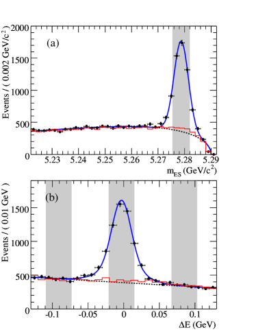
We fit the distribution of the selected candidates with a sum of a Gaussian function for the signal
and a background function for the background having the probability density,
, where with fixed at 5.29 and
is a shape parameter argus2 .
The signal parameters (mean, width of Gaussian) and the shape parameter of the background function are free parameters of the fit.
The data and the result of the fit are shown in Fig. 3a.
We fit the distribution of the selected candidates with a sum of two Gaussian functions with a common mean for the
signal and a linear function for the background.
The signal parameters (mean, width of wide Gaussian, width and fraction of narrow Gaussian)
and the slope of the background function are free parameters of the fit.
The data and the result of the fit are shown in Fig. 3b.
The resulting signal yield is events, where the error is statistical only.
A clear signal is evident in both and distributions.
Figure 3: (a) and (b) distributions for candidates.
Data (points with statistical errors) are compared to the results of the fits (solid curves),
with the background contributions marked as dashed lines.
The histograms are the corresponding distributions of the background MC sample as described in the text.
The shaded area in (a) shows the signal region,
while the three shaded areas in (b) mark the signal region in the center and the two sidebands.
To distinguish signal and background in the Dalitz plot studies,
we divide the candidates into three subsamples:
the signal region, , the left sideband, ,
and the right sideband, .
The events in the signal region are used in the Dalitz plot analysis, while
the events in the sideband regions are used to study the background.
In order to check the shape of the background distribution, we have generated a background MC sample
of resonant and continuum events with signal events removed.
The background MC sample has been scaled to the same luminosity as the data.
The distribution of the selected events from the background MC sample is
shown as the histogram in Fig. 3b.
A small amount of peaking background is found from misreconstructed decays of
with ,
where a is missed and a random track in the event is misidentified as a signal .
The background histogram in Fig. 3b is fitted with a sum of two Gaussian functions with a common mean for the
peaking background, with parameters fixed to those obtained from the fit to data, and a linear function
to describe the combinatorial background. The amount of peaking background is estimated at events.
After peaking background subtraction, the number of signal events above background is .
The background fraction in the signal region is .
IV Dalitz Plot Analysis
We refit the and candidate momenta by
constraining the trajectories of the three daughters of the meson candidate to originate from a common decay vertex
while constraining the invariant masses of and to the and masses PDG , respectively.
The mass-constraints ensure that all events fall within the Dalitz plot boundary.
In the decay of a into
a final state composed of three pseudo-scalar particles (), two
degrees of freedom are required to describe the decay kinematics.
In this analysis we choose the two invariant mass-squared combinations
and as the independent variables, where the two like-sign pions and are randomly assigned to and .
This has no effect on our analysis since the likelihood
function (described below) is explicitly symmetrized with respect
to interchange of the two identical particles.
The differential decay rate is generally given in terms of the Lorentz-invariant matrix element by
(3)
where is the meson mass.
The Dalitz plot gives a graphical representation of the variation of the square
of the matrix element, , over the kinematically accessible phase space (,) of the
process. Non-uniformity in the Dalitz plot can indicate presence of intermediate
resonances, and their masses and spin quantum numbers can be determined.
IV.1 Probability Density Function
We describe the distribution of candidate events in the Dalitz
plot in terms of a probability density function (PDF).
The PDF is the sum of signal and background components and has the form:
where the integral is performed over the whole Dalitz plot,
the is the signal term convolved with the signal resolution function,
is the background term,
is the fraction of background events, and
is the reconstruction efficiency.
An unbinned maximum likelihood fit to the Dalitz plot is performed in order to maximize the value of
(5)
with respect to the parameters used to describe ,
where and are the values of and for event respectively,
and is the number of events in the Dalitz plot.
In practice, the negative-log-likelihood () value
(6)
is minimized in the fit.
IV.2 Goodness-of-fit
It is difficult to find a proper binning at the kinematic
boundaries in the - plane of the Dalitz plot. For this reason, we choose to
estimate the goodness-of-fit in the (range from -1 to 1)
and (range from 4.04 to 15.23 ) plane,
which is a rectangular representation of the Dalitz plot.
The parameter is the helicity angle of the system
and is the lesser of and .
The helicity angle is defined as the angle between the momentum vector of the pion
from the decay (bachelor pion)
and that of the pion of the system in the rest-frame.
The value is calculated using the formula
(7)
for cells in a grid of the two-dimensional histogram.
In Eq. (7),
is the total number of cells used, is the number of events in each cell,
is the expected number of events in that cell as
predicted by the fit results.
The number of degrees of freedom (NDF) is calculated as , where
is the number of free parameters in the fit.
We require ;
if this requirement is not
met then neighboring cells are combined until ten events are accumulated.
IV.3 Matrix element and Fit Parameters
This analysis uses an isobar model formulation in which the signal decays
are described by a coherent sum of
a number of two-body ( system + bachelor pion) amplitudes.
The orbital angular momentum between the system and the bachelor
pion is denoted here as .
The total decay matrix element for is given by:
(8)
where the first term represents the S-wave (), P-wave () and D-wave () nonresonant contributions,
the second term stands for the resonant contributions,
the parameters and are the magnitudes and phases of resonance,
while and correspond to the magnitudes and phases of the nonresonant contributions with angular momentum .
The functions and are the amplitudes for nonresonant and resonant terms, respectively.
The resonant amplitudes are expressed as:
(9)
where is the resonance lineshape,
and are the Blatt-Weisskopf barrier factors formf ,
and gives the angular distribution. The parameter () is the invariant mass of the system.
The parameter is the magnitude of the three momentum of the bachelor pion evaluated in the -meson rest frame.
The parameters and are the magnitudes of the three momenta of the bachelor pion and the pion of the
system, both in the rest frame.
The parameters , , and are functions of and .
The nonresonant amplitudes with are similar to but do not contain resonant mass terms:
(10)
(11)
(12)
The Blatt-Weisskopf barrier factors and
depend on a single parameter, or , the radius of the barrier, which we take to be ,
similarly to Ref. belle-prd .
A discussion of the systematic uncertainty associated with the choice of the values of and follows below.
The forms of , where or , for are:
(13)
(14)
(15)
where or .
Here and represent the values of and , respectively,
when the invariant mass is equal to the pole mass of the resonance.
For nonresonant terms,
the fit results are not affected by the choice of invariant mass (we use the sum of and ) used for the
calculations of and .
For virtual decay, , and virtual production in ,
we use an exponential form factor in place of the Blatt-Weisskopf barrier factor, as discussed in Ref. belle-prd :
(16)
where for and for .
Here, we set , which gives the best fit,
although any value of between 0.015 and gives negligible effect
on the fitted parameters compared to their statistical errors.
The resonance mass term describes the intermediate resonance.
All resonances in this analysis are parametrized with relativistic Breit-Wigner functions:
(17)
where the decay width of the resonance depends on :
(18)
where and are the values of the resonance pole mass and decay width, respectively.
The terms describe the angular distribution of final state particles and
are based on the Zemach tensor formalism Zemach .
The definitions of for are:
(19)
(20)
(21)
The signal function is then given by:
(22)
In this analysis,
the masses of and are taken from the world averages PDG while their widths are fixed at 0.1 ;
the magnitude and phase of the amplitude are fixed to 1 and 0, respectively,
while the masses and widths of resonances and other magnitudes and phases are free parameters to be determined in the fit.
The effect of varying the masses of and within
their errors PDG and widths of and between 0.001 and 0.3 is negligible compared to the other model-dependent systematic uncertainties given below.
Since the choice of normalization, phase convention and amplitude
formalism may not always be the same for different experiments, we use fit fractions and relative phases
instead of amplitudes to
allow for a more meaningful comparison of results. The fit fraction for
the decay mode is defined as the integral of the resonance decay
amplitudes divided by the coherent matrix element squared for the
complete Dalitz plot:
(23)
The fit fraction for nonresonant term with angular momentum has a similar form:
(24)
The fit fractions do not necessarily add up to unity because of interference among the amplitudes.
To estimate the statistical uncertainties on the fit fractions,
the fit results are randomly modified according to the covariance matrix of the fit
and the new fractions are computed using Eq. (23) or (24).
The resulting fit fraction distribution is fitted with a Gaussian whose width gives
the error on the given fraction.
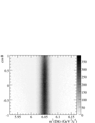
IV.4 Signal Resolution Function
The detector has finite resolution, thus measured quantities differ from their true values.
For the narrow resonance with the expected width of about 40 MeV,
the signal resolution needs to be taken into account.
In order to obtain the signal resolution on around the mass region, we study a sample of MC generated
decays, with the mass and width of set to 2.460 ( mass region)
and 0 MeV, respectively,
and subject these events to the same analysis reconstruction chain.
The reconstructed events are then classified into two categories:
truth-matched (TM) events, where the and the daughters are correctly reconstructed,
and self-crossfeed (SCF) events, where one or more of the daughters is not correctly associated with the generated particle.
The two-dimensional distribution of versus for truth-matched
events is shown in Fig. 4.
Since the resolution is independent of ,
we fit the distribution of the quantity
using a sum of two Gaussian functions with a common mean
to obtain the resolution function for truth-matched events ().
The signal resolution for
an invariant mass of the combination around the region is about 3 .
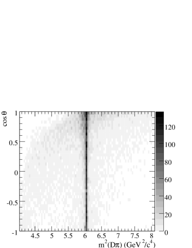
The two-dimensional distribution of versus for
self-crossfeed events is shown in Fig. 5.
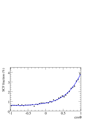
The SCF fraction, , varies from 0.5% to 4.0% with .
We fit the distribution with a 4th-order polynomial function.
The distribution and the result of the fit are shown in Fig. 6.
The resolution for self-crossfeed events varies between 5 and 100 with .
We divide the interval into 40 bins of equal width and use these
bins to describe the resolution function () in terms of a sum of
two bifurcated Gaussian (BGaussian) functions with different means.
The BGaussian is a Gaussian as a function
of with three parameters, the mean, and the two
widths, on the left and on the right side of the mean.
The form of BGaussian is:
(27)
where , and are free parameters.
The signal resolution function is then given by:
(28)
The function represents the probability density
for an event having the true mass squared to be
reconstructed at for different regions.
The signal term in Eq. (LABEL:pdfall) is convoluted with the above resolution function.
For each event, the convolution is performed using numerical integration:
(29)
where is the signal function in Eq. (22), and ()
is the lesser (greater) of and .
The quantity is determined from and and is assumed to be
constant during convolution.
The resolution in has a negligible effect on the fitted parameters.
The quantity is computed using the kinematics
of three-body decay with , and .
The resolution function and the integration method in Eq. (29) have been
fully tested using 262 MC samples with full event reconstruction given below.
We have compared invariant mass resolutions for ,
and between data and MC-simulated events
and find that they agree within their statistical uncertainties.
Estimated biases in the fitted parameters due to
uncertainties in the signal resolution function are small and have
been included into the systematic errors.
Figure 4: Two-dimensional histogram versus of the
truth-matched events as defined in the text.Figure 5: Two-dimensional histogram versus of the
self-crossfeed events as defined in the text.Figure 6: distribution.
The observed self-crossfeed fractions (points with statistical errors) are compared to the results of the fit (solid curve).
IV.5 Efficiency
The signal term defined above is modified in order to take into account experimental particle
detection and event reconstruction efficiency.
Since different regions of the Dalitz plot correspond to different event topologies, the efficiency is not
expected to be uniform over the Dalitz plot.
The term in Eq. (LABEL:pdfall) is the overall efficiency for truth-matched and self-crossfeed signal events,
hence the efficiency for truth-matched signal events is
(30)
In order to determine the efficiency across the Dalitz plot,
a sample of simulated events in the Dalitz plot is generated.
Some events are generated with one or more additional final-state photons
to account for radiative corrections radiative .
As a result, the generated Dalitz plot is slightly distorted from the uniform distribution.
The number of generated events is
1252k. Each event is subjected to
the standard reconstruction and selection, described in Section III.
In addition, we require that the candidate decay is truth matched.
After correcting for data/MC efficiency differences in particle identification,
which are momentum dependent and thus vary over the Dalitz plot,
the total number of accepted events is
. We employ an unbinned likelihood method
to fit the Dalitz plot distributions for generated and accepted event samples.
The PDF for generated events () is a fourth-order two-dimensional polynomial
while the PDF for accepted events () is a seventh-order
two-dimensional polynomial. The efficiency function is then given by:
(31)
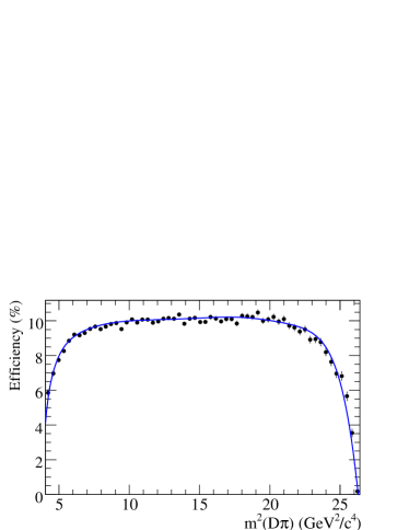
Fig. 7 shows the efficiency as a function of and the fit result for MC-simulated events.
Figure 7: The efficiency for signal decays as a function of , as determined by MC
simulation (points with statistical errors) and the results of the fit to the
accepted and generated distributions (solid curve).
IV.6 Background
The background distribution is modeled using
MC background events, selected with the same criteria
applied to the data and requiring the candidate to fall into the signal
region defined in Section III.
Events in the data sidebands could also be used to model the background, however in MC
studies we find differences between the Dalitz plot distributions of the
background in the signal and sideband regions. Since we find the Dalitz
plot distributions of sideband events in data and in MC simulation to be
consistent within their statistics, we are confident that the MC simulation can accurately represent the
background distribution in the signal region.
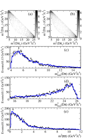
Fig. 8a, 8b and Fig. 9a show the
Dalitz plot distributions of sideband events in data, sideband events in the MC sample
and background events in the signal region of the MC sample, respectively.
Fig. 8c, 8d and 8e show the comparisons
of sideband events between data and MC simulation in
, and projections, respectively.
Here () is the lesser (greater) of and .
Figure 8: Comparison of events in the sideband:
Dalitz plot for (a) data and (b) MC-simulated events,
and projections on (c) , (d) and
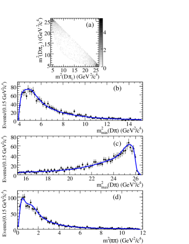
(e) with data (points with statistical errors) and MC predictions (histograms).Figure 9: Fit to background events in the signal region of the MC sample:
(a) Dalitz plot and projections on (b) , (c) and
(d) with MC predictions (points with statistical errors) and
the fits (solid curves).
The parameterization used to describe the background is:
(32)
where the coefficients to are free parameters to be
determined from the fit, and
are the lower and upper limits of the
Dalitz plot, respectively, is the lower
limit of , is the lesser of and
, is the greater of and , is the
invariant , and is given in Eq. (27).
The projections on , and and the
result of the fit for the background events in the signal region of the MC sample
are shown in Fig. 9b, 9c
and 9d.
The for the fit is .
V Results
V.1 Branching Fraction
The total branching fraction is calculated using the relation:
(33)
where is the fitted signal yield given in Section III,
is the average efficiency,
% is the branching fraction for PDG ; cleodpp ,
and the total number of events, ,
is determined using and the ratio of () PDG .
Since the reconstruction efficiencies vary slightly for different resonances,
the average efficiency is calculated by weighing the
accepted and generated events by with the values for the parameters of
our nominal Dalitz plot model (discussed below):
(34)
where is the correction factor which depends on and due to particle identification efficiency.
The value % is obtained using this method.
The measured total branching fraction is
,
where the stated error refers to the statistical uncertainty only.
A full discussion of the systematic uncertainties follows below.
V.2 Dalitz plot analysis results
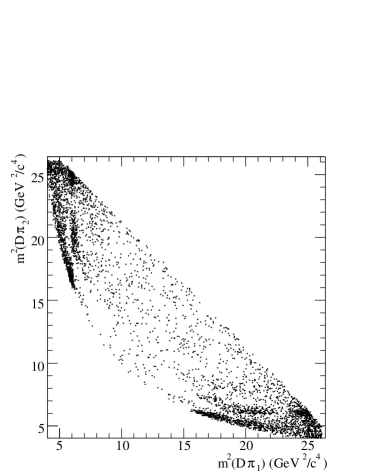
The Dalitz plot distribution for data is shown in Fig. 10.
Since the composition of events in the Dalitz plot and their distributions are not
known a priori, we have
tried a variety of different assumptions. In particular,
we test the inclusion of various components,
such as the virtual and as well as S-, P- and D-wave modeling of the nonresonant component,
in addition to the expected components of , and background.
The D-wave nonresonant term does not improve the goodness-of-fit and the fraction of D-wave nonresonant contribution
is close to 0.
The results of these tests with variations of the models are summarized in Table 2.
Table 2: Fit results for the masses, widths, fit fractions and phases from the Dalitz plot analysis
of for different models. The errors are statistical only.
The magnitude and phase of the amplitude are fixed to 1 and 0, respectively.
The background fraction is fixed to 30.4% as described in Section III.
The nominal fit corresponds to model 1.
The labels, S-NR and P-NR, denote the S-wave nonresonant and P-wave nonresonant contributions, respectively.
Parameter
Model 1
Model 2
Model 3
Model 4
Model 5
Model 6
Model 7
()
()
()
()
(%)
(rad)
0.0 (fixed)
0.0 (fixed)
0.0 (fixed)
0.0 (fixed)
0.0 (fixed)
0.0 (fixed)
0.0 (fixed)
(%)
(rad)
(%)
(rad)
(%)
(rad)
(%)
(rad)
(%)
(rad)
(%)
(fixed)
(fixed)
(fixed)
(fixed)
(fixed)
(fixed)
(fixed)
NLL
22970
22982
22977
22982
22964
23046
23125
Of these models, model 1 produces the best fit quality with the smallest number of components,
and we choose it as the nominal fit model.
The components considered in this fit model are
, , , and P-wave nonresonant.
The P-wave nonresonant component is an addition to the fit model used in the previous measurement from Belle belle-prd .
The sum of the fractions ()% for the nominal fit
differs from 100% because of destructive interferences among the amplitudes.
The for the nominal fit is .
To better understand the large , we look at the contributions to
the total from individual cells. We find four cells with , which inflate the
total . The central points in these cells are at: (), (), ()
and (), where the first value is , and the second is .
In order to determine the effect on the fitted parameters from these cells, we repeat the nominal
fit with these cells excluded.
The resulting is , corresponding to a probability of 3.4%.
Assuming these large contributions are caused by an unknown
systematic problem, removing them from the fit is reasonable.
However, under the assumption that these high contributions
have a statistical origin, the probability is 0.04% prob .
The low probability indicates that a model more complex than the
isobar model may be necessary to describe the characteristics of the data.
The differences in the fitted and parameters, when these cells are
included or excluded, are assigned to systematic uncertainties,
and are much smaller than the statistical uncertainties.
The removal of these cells does not affect the choice of model 1
as the nominal fit from Table 2.
Ref. dpi argues for an addition of a S-wave state near the
system threshold to the model of the final state.
We have performed tests using the models 1-4
in Table 2 with the replaced by a S-wave state.
Two different parametrizations for S-wave state amplitude are used:
one is the function given by Eq.(8) of Ref. dpi with
the numerator set to constant,
the other function is the relativistic Breit-Wigner given by Eq. (17).
Among the tests we have performed with these parameterizations,
the model with , ,
S-wave (using Eq.(8) of Ref. dpi ), and
P-wave nonresonant gives the best fit with NLL and values
of 22997 and , respectively, which are worse than those of the nominal fit
even when allowing the S-wave’s parameters to vary.
Each of these models also requires large fractions of .
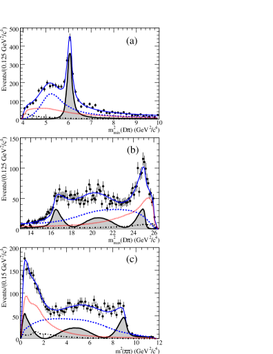
Figure 10: Data Dalitz Plot for .Figure 11: Result of the nominal fit to the data: projections on
(a) , (b) and (c) .
The points with error bars are data, the solid curves represent the nominal fit.
The shaded areas show the contribution,
the dashed curves show the signal, the dash-dotted curves show the and signals,
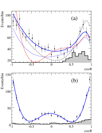
and the dotted curves show the background.Figure 12: Result of the nominal fit to the data: the distributions for
(a) region and
(b) region.
The points with error bars are data, the solid curves represent the nominal fit.
The dashed, dash-dotted and dotted curves in (a) show the fit of hypotheses 2-4 in Table 3, respectively.
The shaded histograms
show the distributions from sidebands in data.
The nominal fit model results in the following branching fractions:
and
,
where the errors are statistical only.
A full discussion of the systematic uncertainties follows below.
Fig. 11a, 11b and 11c show the
, and projections respectively,
while Fig. 12a and 12b show the
distributions for the and mass regions, respectively.
The distributions in Fig. 11 and 12 show good agreement between the data and the fit.
The angular distribution in the mass region
is clearly visible and is consistent with the expected D-wave distribution of for a spin-2 state.
In addition, the signal and the reflection of
can be easily distinguished in the and projection, respectively.
The lower edge of is better described with component included than without.
Table 3 shows the NLL and values for the nominal fit and
for the fits with the broad resonance excluded or with the
of the broad resonance replaced by other quantum numbers.
In all cases, the NLL and values are significantly worse than that of the nominal fit.
Fig. 12a illustrates the helicity distributions in the mass region
from hypotheses 2-4; clearly the nominal fit gives the best description of the data.
We conclude that a broad spin-0 state is required in the fit to the data.
The same conclusion is obtained when performing the
same test on Models 2-5.
Table 3: Comparison of the models with different resonances composition.
The labels, S-NR and P-NR, denote the S-wave nonresonant and P-wave nonresonant contributions, respectively.
Hypothesis
Model
NLL
Model 1 (nominal fit)
22970
1
, P-NR
23761
2
, P-NR,
23699
3
, P-NR,
23427
4
, P-NR, S-NR
23339
VI SYSTEMATIC UNCERTAINTIES
VI.1 Uncertainties on
As listed in Table IV, the systematic
error on the measurement of the total branching fraction is due to the uncertainties on the following quantities:
the number of events in the initial sample, the charged track reconstruction and identification efficiencies,
and the branching fraction. The uncertainty in the background shape, the uncertainty in the average efficiency
due to the fit models and
a possible fit bias also contribute to the systematic error.
Table 4: Summary of systematic uncertainties (relative errors in %) in the measurement of the total branching fraction.
Systematic Source
(%)
Number of events
Tracking efficiencies
PID
background shape
branching fraction
Fit models
Fit bias
Total Systematics
The uncertainty on the number of events is determined using the uncertainties on
PDG and integrated luminosity (1.1%).
The uncertainty on the input branching fraction is taken
from cleodpp .
The uncertainty in the background shape
is estimated by comparing the signal yields between fitting the distribution
with a linear background shape and with higher-order (second and third-order) polynomials.
The uncertainty in the fit models is estimated by comparing the average efficiencies in Eq. (34) using
Models 2-5 of Table 2.
The fit bias is estimated to be less than 1% by comparing
the generated and the fitted value of from resonant and continuum MC samples.
VI.2 Uncertainties on Dalitz plot analysis results
The sources of systematic uncertainties that affect the results of the Dalitz Plot analysis
are summarized in Table V.
These uncertainties are added in quadrature, as they are uncorrelated, to obtain the total systematic error.
The uncertainties due to the background
parameterization are estimated by comparing the results from the nominal
fit with those obtained when the background shape parameters are allowed
to float in the fit.
The errors from the uncertainty in the background fraction are estimated by comparing
the fit results when the background fraction is changed by its statistical error.
We vary the set of cuts on , , ,
and mass of , which increase the number of signal events by 25%
and the background fraction to 36.5%, and repeat the fits.
The difference in the fit results is taken as an estimate of the systematic uncertainty due to the event selection.
Fit biases are studied using 1248 parameterized MC samples and
262 MC samples with full event reconstruction.
Small biases are observed for some of the parameters.
We combine these biases with those coming from high
cells, as discussed in the previous section, in quadrature to obtain the
total systematic contribution from the fit bias.
The uncertainties in PID are obtained by comparing the nominal fit results with those obtained when
the PID corrections to the reconstruction efficiency are varied according to their uncertainties.
The uncertainties in the efficiency and signal resolution parametrization
are found to be negligible using the fits to the reconstructed MC samples.
In addition to the above systematic uncertainties, we also estimate a
model-dependent uncertainty that comes from the uncertainty in the composition of the signal model and
the uncertainty in the Blatt-Weisskopf barrier factors.
The model-dependent uncertainties are estimated by comparing the fit results with
Models 2-5 in Table 2
and by varying the radius of the barrier, and in Eqs. (14)-(16)
from 0 to 5 .
Table 5: Summary of systematic uncertainties in the masses, widths and fit fractions of the and and the phase of .
Systematic Source
()
()
()
()
(%)
(%)
(rad)
Background parameterization
1.0
1.1
3
5
1.2
0.0
0.04
Background fraction
0.1
0.4
2
1
0.4
0.4
0.00
Event selection
0.6
1.6
1
14
0.3
0.8
0.08
Fit bias
0.3
0.7
4
8
0.7
1.4
0.02
PID efficiency
0.0
0.1
0
0
0.0
0.1
0.01
Total systematic error
1.2
2.1
5
17
1.5
1.7
0.09
Fit models
1.3
0.7
15
40
1.5
17.2
0.07
constant
1.4
1.9
12
21
3.8
7.8
0.17
Total model-dependent error
1.9
2.0
19
45
4.1
18.9
0.18
VII SUMMARY
In conclusion, we measure
the total branching fraction of the decay to be
where the first error is statistical and the second is
systematic.
Analysis of the Dalitz plot using the isobar model confirms the existence
of a narrow and a broad resonance as predicted by Heavy Quark Effective Theory.
The mass and width of are determined to be:
respectively, while for the they are:
where the first and second errors reflect the statistical
and systematic uncertainties, respectively, the third one
is the uncertainty related to the assumed composition of signal events
and the Blatt-Weisskopf barrier factors.
The measured masses and widths of both states are consistent
with the world averages PDG and the predictions of some theoretical models isgur ; ebert ; kalashnikova .
We have also obtained exclusive branching fractions for and production:
Our results for the masses, widths and branching fractions are consistent
with but more precise than previous measurements performed by Belle belle-prd .
The relative phase of the scalar and tensor amplitude is measured to be
Acknowledgements.
We are grateful for the
extraordinary contributions of our PEP-II colleagues in
achieving the excellent luminosity and machine conditions
that have made this work possible.
The success of this project also relies critically on the
expertise and dedication of the computing organizations that
support BABAR.
The collaborating institutions wish to thank
SLAC for its support and the kind hospitality extended to them.
This work is supported by the
US Department of Energy
and National Science Foundation, the
Natural Sciences and Engineering Research Council (Canada),
the Commissariat à l’Energie Atomique and
Institut National de Physique Nucléaire et de Physique des Particules
(France), the
Bundesministerium für Bildung und Forschung and
Deutsche Forschungsgemeinschaft
(Germany), the
Istituto Nazionale di Fisica Nucleare (Italy),
the Foundation for Fundamental Research on Matter (The Netherlands),
the Research Council of Norway, the
Ministry of Education and Science of the Russian Federation,
Ministerio de Educación y Ciencia (Spain), and the
Science and Technology Facilities Council (United Kingdom).
Individuals have received support from
the Marie-Curie IEF program (European Union) and
the A. P. Sloan Foundation.
References
(1) N. Isgur and M. B. Wise, Phys. Lett. B 232, 113 (1989).
(2) M. Neubert, Phys. Rept. 245, 259 (1994).
(3) A. F. Falk and M. Luke, Phys. Lett. B 292, 119 (1992).
(4) A. F. Falk and M. E. Peskin, Phys. Rev. D 49, 3320 (1994).
(5) Particle Data Group, C. Amsler et al., Phys. Lett. B 667, 1 (2008).
(6) ARGUS Collaboration, H. Albrecht et al., Phys. Lett. B 232, 398 (1989).
(7) Tagged Photon Spectrometer Collaboration, J. C. Anjos et al., Phys. Rev. Lett. 62, 1717 (1989).
(8) CLEO Collaboration, P. Avery et al., Phys. Rev. D 41, 774 (1990).
(9) CLEO Collaboration, T. Bergfeld et al., Phys. Lett. B 340, 194 (1994).
(10) E687 Collaboration, P. L. Frabetti et al., Phys. Rev. Lett. 72, 324 (1994).
(11) CLEO Collaboration, P. Avery et al., Phys. Lett. B 331, 236 (1994).
(12)
Belle Collaboration, K. Abe et al., Phys. Rev. D 69, 112002 (2004).
(13) FOCUS Collaboration, J. M. Link et al., Phys. Lett. B 586, 11 (2004).
(14)
Belle Collaboration, K. Abe et al., Phys. Rev. Lett. 94, 221805 (2005).
(15) CDF Collaboration, A. Abulencia et al., Phys. Rev. D 73, 051104 (2006).
(16)
Belle Collaboration, A. Kuzmin et al., Phys. Rev. D 76, 012006 (2007).
(17) ALEPH Collaboration, D. Buskulic et al., Z. Phys. C 73, 601 (1997).
(18) CLEO Collaboration, A. Anastassov et al., Phys. Rev. Lett. 80, 4127 (1998).
(19) D0 Collaboration, V. M. Abazov et al., Phys. Rev. Lett. 95, 171803 (2005).
(20) DELPHI Collaboration, J. Abdallah et al., Eur. Phys. J. C 45, 35, (2006).
(21)BABAR Collaboration, B. Aubert et al., Phys. Rev. D 76, 051101 (2007).
(22)
Belle Collaboration, D. Liventsev et al., Phys. Rev. D 77, 091503 (2008).
(23)BABAR Collaboration, B. Aubert et al., arXiv:0808.0333 [hep-ex], submitted to Phys. Rev. Lett.
(24)BABAR Collaboration, B. Aubert et al., Phys. Rev. Lett. 101, 261802 (2008).
(25)
M. Kobayashi and T. Maskawa, Prog. Theor. Phys. 49, 652 (1973).
(26) Charged conjugate states are implied throughout the paper.
(27) GEANT4 Collaboration, S. Agostinelli et al., Nucl. Instrum. Methods Phys. Res., Sect. A 506, 250 (2003).
(28) D. J. Lange, Nucl. Instrum. Methods Phys. Res., Sect. A 462, 152 (2001).
(29) T. Sjöstrand, Comput. Phys. Commun. 82, 74 (1994).
(30)BABAR Collaboration, B. Aubert et al., Nucl. Instrum. Methods A 479, 1 (2002).
(31) G. C. Fox and S. Wolfram, Phys. Rev. Lett. 41, 1581 (1978).
(32) ARGUS Collaboration, H. Albrecht et al., Z. Phys. C 48, 543 (1990).
(33) J. Blatt and V. Weisskopf, Theoretical Nuclear Physics, p.361, New York: John Wiley & Sons (1952).
(34) C. Zemach, Phys. Rev. 140, B97 (1965).
(35) E. Barberio and Z. Was, Comp. Phys. Commun. 79, 291 (1994).
(36) CLEO Collaboration, S. Dobbs et al., Phys. Rev. D 76, 112001 (2007).
(37) 0.04% is the probability to obtain a of 182 or greater
for a collection of 153 standard normal-distributed numbers,
of which the four largest positive deviations have been removed.
(38) D. V. Bugg, arXiv:0901.2217 [hep-ph], to be published in J. Phys. G: Nucl. Part. Phys.
(39) N. Isgur, Phys. Rev. D 57, 4041 (1998).
(40) D. Ebert, V. O. Galkin and R.N. Faustov, Phys. Rev. D 57, 5663 (1998).
(41) Y. S. Kalashnikova and A. V. Nefediev, Phys. Lett. B 530, 117 (2002).