On ²²⁹Th and time-dependent fundamental constants

Abstract

The electromagnetic transition between the almost degenerate 5/2⁺ and $3/2^{+}$ states in ²²⁹Th is deemed to be very sensitive to potential changes in the fine structure constant $\alpha$. State of the art Hartree-Fock and Hartree-Fock-Bogoliubov calculations are performed to compute the difference in Coulomb energies of the two states which determines the amplification of variations in $\alpha$ into variations of the transition frequency. The kinetic energies are also calculated which reflect a possible variation in the nucleon or quark masses. A generalized Hellmann–Feynman theorem is proved including the use of density-matrix functionals. As the two states differ mainly in the orbit occupied by the last unpaired neutron the Coulomb energy difference results from a change in the nuclear polarization of the proton distribution. This effect turns out to be rather small and to depend on the nuclear model, the amplification varies between about $-4\times 10^{4}$ and $+4\times 10^{4}$. Therefore much more effort must be put into the improvement of the nuclear models before one can draw conclusions from a measured drift in the transition frequency on a temporal drift of fundamental constants. All calculations published so far do not reach the necessary fidelity.

I Introduction

Measurements of a suspected temporal variation of the fine structure constant by means of atomic transitions have reached an limit for $\delta\alpha/\alpha$ of less than $10^{-16}\mathrm{yr}^{-1}$ Rosenband et al. (2008); Fortier et al. (2007); Peik et al. (2004); Fischer et al. (2004); Prestage et al. (1995); Flambaum (2008).

A tempting idea to increase the sensitivity limit is to use the transition between two states with very different Coulomb energies, because the drift in transition frequency

$$\frac{\delta\omega}{\omega}=A\;\frac{\delta\alpha}{\alpha}\ \ \ \mathrm{with}\ \ \ A=\frac{\Delta V_{C}}{\omega}$$ (1)

is given by an amplification factor $A$ times the drift in $\alpha$. Using the Hellmann–Feynman theorem $A$ is the ratio of the difference $\Delta V_{C}$ in Coulomb energies of the two states involved in the transition divided by the transition frequency $\omega$. A promising candidate for that is the transition between the $3/2^{+}$ isomeric state of the nucleus ²²⁹Th to its $5/2^{+}$ ground state Peik and Tamm (2003); Flambaum (2006). Recent measurements yield $\omega=7.6\pm 0.5$ eV Beck et al. (2007) which on nuclear energy scales is an accidental almost degeneracy. Typical Coulomb energies for this nucleus are of the order of $V_{C}\approx 10^{9}$ eV so that even a small difference $\Delta V_{C}$ could result in a large amplification.

A big drawback of this idea is that the Coulomb energies cannot be measured but have to be calculated with sufficient accuracy in a nuclear model. Differences in charge radii and quadrupole moments of the nuclear states are in principle experimentally accessible. Their measurement would reduce the uncertainty.

In a simplified picture the two states differ by the occupation of the last neutron orbit. The change in the Coulomb energy is thus due to a modified neutron distribution in the excited state that will polarize via the strong interaction the proton distribution in a slightly different way than in the ground state.

In this paper we investigate in how far state of the art nuclear models can provide reliable answers. For that in section II we revisit first the Hellmann–Feynman theorem proposed by H. Hellmann Hellmann (1933) and also by R. Feynman Feynman (1933) and show that it is also valid in a wider context including density-matrix functional theory employed in nuclear physics. After introducing the nuclear models in Sec. III we discuss in Sec. IV the amplification of the temporal drift of fundamental constants like the fine structure constant or the nucleon mass when monitoring transition frequencies.

For the nuclear candidate ²²⁹Th we perform in Sec. V self-consistent nuclear structure calculations and determine via the Hellmann–Feynman theorem the derivatives of the transition frequency with respect to the fine structure constant and the nucleon mass. A critical assessment is made on the predictive power when calculating observables other than the energy. Finally we summarize.

II Hellmann–Feynman theorem revisited

In this section we show that the Hellmann–Feynman theorem holds not only for eigenstates of the Hamiltonian but also for all stationary solutions in approximate schemes, provided they are variational. This is of importance as the models we are using are based on density-matrix functionals.

Let the Hamiltonian $H(\mathbf{c})$ depend on a set of external parameters $\mathbf{c}=\{c_{1},c_{2},\dots\}$, like the strength of an interaction or the mass of the particles. The steady state solutions of the time-dependent Schrödinger equation are given by the eigenvalue problem

$$H(\mathbf{c})\big{|}\,{\Psi_{n};\mathbf{c}}\,\big{>}=E_{n}(\mathbf{c})\big{|}\,{\Psi_{n};\mathbf{c}}\,\big{>}\ .$$ (2)

Both, the energies $E_{n}(\mathbf{c})$ and the eigenstates $\big{|}\,{\Psi_{n};\mathbf{c}}\,\big{>}$ depend on $\mathbf{c}$. When discussing intermolecular forces in 1933 H. Hellmann Hellmann (1933) and later in 1939 R. P. Feynman Feynman (1933) showed that a small variation of an external parameter in the Hamiltonian (distance between nuclei) leads to a change in the energy given by:

$$\frac{\partial{}}{\partial{c_{i}}}E_{n}(\mathbf{c})=\frac{\big{<}\,{\Psi_{n};\mathbf{c}}\,\big{|}\,{\frac{\partial{}}{\partial{c_{i}}}H(\mathbf{c})}\,\big{|}\,{\Psi_{n};\mathbf{c}}\,\big{>}}{\big{<}\,{\Psi_{n};\mathbf{c}}\,\big{|}\,{\Psi_{n};\mathbf{c}}\,\big{>}}\ .$$ (3)

The proof hinges on $\big{|}\,{\Psi_{n};\mathbf{c}}\,\big{>}$ being an eigenstate of the hermitian $H(\mathbf{c})$:

$$\frac{\partial{}}{\partial{c_{i}}} E_{n}(\mathbf{c})=\frac{\partial{}}{\partial{c_{i}}}\frac{\big{<}\,{\Psi_{n};\mathbf{c}}\,\big{|}\,{H(\mathbf{c})}\,\big{|}\,{\Psi_{n};\mathbf{c}}\,\big{>}}{\big{<}\,{\Psi_{n};\mathbf{c}}\,\big{|}\,{\Psi_{n};\mathbf{c}}\,\big{>}}$$

$$\!\!=\frac{\big{<}\,{\Psi_{n};\mathbf{c}}\,\big{|}\,{\frac{\partial{}}{\partial{c_{i}}}H(\mathbf{c})}\,\big{|}\,{\Psi_{n};\mathbf{c}}\,\big{>}}{\big{<}\,{\Psi_{n};\mathbf{c}}\,\big{|}\,{\Psi_{n};\mathbf{c}}\,\big{>}}$$ (4)

$$\!\!+\left[\frac{\big{<}\,{\frac{\partial{\Psi_{n}}}{\partial{c_{i}}};\mathbf{c}}\,\big{|}\,{H(\mathbf{c})}\,\big{|}\,{\Psi_{n};\mathbf{c}}\,\big{>}}{\big{<}\,{\Psi_{n};\mathbf{c}}\,\big{|}\,{\Psi_{n};\mathbf{c}}\,\big{>}}\ +\ h.a.\right]$$

$$\!\!-\left[\frac{\big{<}\,{\Psi_{n};\mathbf{c}}\,\big{|}\,{H(\mathbf{c})}\,\big{|}\,{\Psi_{n};\mathbf{c}}\,\big{>}}{\big{<}\,{\Psi_{n};\mathbf{c}}\,\big{|}\,{\Psi_{n};\mathbf{c}}\,\big{>}}\frac{\big{<}\,{\frac{\partial{\Psi_{n}}}{\partial{c_{i}}};\mathbf{c}}\,\big{|}\,{\Psi_{n};\mathbf{c}}\,\big{>}}{\big{<}\,{\Psi_{n};\mathbf{c}}\,\big{|}\,{\Psi_{n};\mathbf{c}}\,\big{>}}\ +\ h.a.\right].$$

Inserting (2) in the terms enclosed in square brackets leads to a cancellation of these terms and we are left with Eq. (3), the Hellmann–Feynman theorem. The partial derivative of any eigenvalue $E_{n}(\mathbf{c})$ with respect to a parameter $c_{i}$ is equal to the expectation value of the partial derivative of the Hamiltonian calculated with the corresponding eigenstate $\big{|}\,{\Psi_{n};\mathbf{c}}\,\big{>}$.

We now show that the same statement holds for any extremal point in an energy functional. Let ${\cal E}(\mathbf{c},\mathbf{x})$ be the energy of a physical system that depends on external parameters $\mathbf{c}$ and on a set of variational parameters $\mathbf{x}=\{x_{1},x_{2},\cdots\}$ which characterize the state of the system. $\mathbf{x}$ may also represent a set of functions in which case partial derivatives are replaced by functional derivatives.

For example, in the Hartree-Fock approximation $\mathbf{x}$ would be the set of occupied single-particle states that form a Slater determinant. In an energy density functional $\mathbf{x}$ could be the local density $\rho(\!\vec{\,r})$, and so on.

Steady state solutions $\mathbf{x}^{(n)}(\mathbf{c}),\ n=0,1,2,\dots$ of the system are obtained by the condition

$$0=\frac{\partial{{\cal E}}}{\partial{x_{k}}}(\mathbf{c},\mathbf{x})$$ (5)

At the stationary points the energy assumes the values

$$E_{n}(\mathbf{c})={\cal E}(\mathbf{c},\mathbf{x}^{(n)}(\mathbf{c})),\ \ \ n=0,1,2,\dots\ .$$ (6)

Both, the energies and the parameters $\mathbf{x}^{(n)}(\mathbf{c})$ characterizing the stationary states depend on the constants $\mathbf{c}$. In the ground state given by $\mathbf{x}^{(0)}$ the energy ${\cal E}(\mathbf{c},\mathbf{x})$ is in an absolute minimum with respect to variations in $\mathbf{x}$, while the other possible solutions $\mathbf{x}^{(n)},n\neq 0$, represent saddle points.

A variation of the external parameters at the stationary points leads to

$$\delta E_{n}(\mathbf{c}) =\sum_{i}\frac{\partial{}}{\partial{c_{i}}}E_{n}(\mathbf{c})\,\delta c_{i}$$ (7)

$$=\sum_{i}\Big{[}\frac{\partial{{\cal E}}}{\partial{c_{i}}}\big{(}\mathbf{c},\mathbf{x}^{(n)}(\mathbf{c})\big{)}\ +$$

$$\hskip 50.00008pt\sum_{k}\frac{\partial{{\cal E}}}{\partial{x_{k}}}\big{(}\mathbf{c},\mathbf{x}^{(n)}(\mathbf{c})\big{)}\ \frac{\partial{x^{(n)}_{k}}}{\partial{c_{i}}}(\mathbf{c})\Big{]}\,\delta c_{i}\ .$$

Due to the stationarity condition (5) the second part in the square brackets vanishes so that we obtain for stationary solutions

$$\frac{\partial}{\partial{c_{i}}}\ E_{n}(\mathbf{c})=\frac{\partial{\cal E}}{\partial c_{i}} \big{(}\mathbf{c},\mathbf{x}^{(n)}(\mathbf{c})\big{)}\ .$$ (8)

The derivative of the energy at the stationary solutions is just the partial derivative of the energy functional with respect to the external parameter calculated with the stationary state. This generalizes the Hellmann–Feynman theorem (3).

Taking

$${\cal E}(\mathbf{c},\mathbf{x})=\frac{\big{<}\,{\mathbf{x}}\,\big{|}\,{H(\mathbf{c})}\,\big{|}\,{\mathbf{x}}\,\big{>}}{\big{<}\,{\mathbf{x}}\,\big{|}\,{\mathbf{x}}\,\big{>}}\ \ \mbox{and}\ \ \big{|}\,{\mathbf{x}}\,\big{>}=\sum_{k}x_{k}\big{|}\,{k}\,\big{>}\ ,$$ (9)

where $\big{|}\,{k}\,\big{>}$ denotes some fixed basis and doing a variation with respect to the parameters $\mathbf{x}=\{x_{1},x_{2},\dots\}$ yields the time-independent Schrödinger equation (2) and the original Hellmann–Feynman theorem (3) as a special case of (8).

It is interesting to note that the Hellmann–Feynman theorem even applies to every solution $\big{|}\,{\Psi(t)}\,\big{>}$ of the time-dependent Schrödinger equation

$$i\frac{d}{dt}\big{|}\,{\Psi(t)}\,\big{>}=H\big{(}\mathbf{c}(t)\big{)}\ \big{|}\,{\Psi(t)}\,\big{>}\ .$$ (10)

For the total time derivative of the mean energy, which is the expectation value of the Hamiltonian, one obtains

$$\frac{dE}{dt}= \frac{d}{dt}\frac{\big{<}\,{\Psi(t)}\,\big{|}\,{H\big{(}\mathbf{c}(t)\big{)}}\,\big{|}\,{\Psi(t)}\,\big{>}}{\big{<}\,{\Psi(t)}\,\big{|}\,{\Psi(t)}\,\big{>}}$$

$$= \sum_{i}\frac{\big{<}\,{\Psi(t)}\,\big{|}\,{\frac{\partial{}}{\partial{c_{i}}}H\big{(}\mathbf{c}(t)\big{)}}\,\big{|}\,{\Psi(t)}\,\big{>}}{\big{<}\,{\Psi(t)}\,\big{|}\,{\Psi(t)}\,\big{>}}\ \frac{d\,c_{i}}{dt}(t)$$

$$+\left[\frac{\big{<}\,{\Psi(t)}\,\big{|}\,{H\big{(}\mathbf{c}(t)\big{)}\frac{d}{dt}}\,\big{|}\,{\Psi(t)}\,\big{>}}{\big{<}\,{\Psi(t)}\,\big{|}\,{\Psi(t)}\,\big{>}}\ +\ h.a.\right]\ .$$ (11)

Here we used the fact that a hermitian Hamiltonian does not change the norm of the state $\big{|}\,{\Psi(t)}\,\big{>}$. Inserting the time-dependent Schrödinger equation (10) into the expression in the square brackets lets this term of the equation vanish so that the time-dependent Hellmann–Feynman theorem reads:

$$\frac{dE}{dt}= \sum_{i}\frac{\big{<}\,{\Psi(t)}\,\big{|}\,{\frac{\partial{}}{\partial{c_{i}}}H\big{(}\mathbf{c}(t)\big{)}}\,\big{|}\,{\Psi(t)}\,\big{>}}{\big{<}\,{\Psi(t)}\,\big{|}\,{\Psi(t)}\,\big{>}}\ \frac{d\,c_{i}}{dt}(t)\ .$$ (12)

Again the variation of the energy is given by the expectation value of the derivatives of the Hamiltonian with respect to the external parameters. See also Ref. Di Ventra and Pantelides (2000).

The generalized theorem (8) is even valid for classical mechanics, just take $\mathbf{x}$ to be the canonical variables $p$ and $q$. The equations of motion are

$$\frac{d\,p}{dt}=-\frac{\partial{{\cal E}}}{\partial{q}}(\mathbf{c},p,q)\ \ \mbox{and}\ \ \frac{d\,q}{dt}=\frac{\partial{{\cal E}}}{\partial{p}}(\mathbf{c},p,q)\ .$$ (13)

At the stationary points the partial derivatives of the Hamilton function ${\cal E}(\mathbf{c},p,q)$ vanish and one obtains again Eq. (8).

III Models

In this section we discuss briefly the Hartee-Fock (HF) method when a Hamiltonian is used, the extension to HF with density-matrix functionals and the inclusion of pairing correlations. We show that in all cases the generalized Hellmann–Feynman relation holds. We also explain in short the quantities discussed in the section containing calculations for ²²⁹Th.

III.1 Hartree-Fock with Hamiltonian

In the HF approximation one uses a single Slater determinant

$$\big{|}\,{\Psi_{\mathrm{HF}}}\,\big{>}=a^{\dagger}_{1}\,a^{\dagger}_{2}\,\cdots a^{\dagger}_{A}\,\big{|}\,{\emptyset}\,\big{>}$$ (14)

as the many-body trial state. The creation operators $a^{\dagger}_{\nu}$ that create the occupied single-particle states $\big{|}\,{\phi_{\nu}}\,\big{>}$,

$$a^{\dagger}_{\nu}\>\big{|}\,{\emptyset}\,\big{>}=\big{|}\,{\phi_{\nu}}\,\big{>}=\sum_{i}c^{\dagger}_{i}\>\big{|}\,{\emptyset}\,\big{>}\>D_{i\nu}\ ,$$ (15)

are represented in a working basis $\big{|}\,{i}\,\big{>}=c^{\dagger}_{i}\>\big{|}\,{\emptyset}\,\big{>}$. Thus, the expansion coefficients $D_{i\nu}$ represent the set $\boldsymbol{x}=\{D_{i\nu};\nu=1,\dots,A,i=1,2,\dots\}$ of variational parameters.

The general definition of the one-body density operator

$$\hat{\rho}=\sum_{i,k}\big{|}\,{i}\,\big{>}\>\rho_{ik}\>\big{<}\,{k}\,\big{|}$$ (16)

is given in terms of the expectation values of $c^{\dagger}_{k}c_{i}$, where the creation operators $c^{\dagger}_{i}$ create the single-particle basis $\big{|}\,{i}\,\big{>}$. In the HF case:

$$\rho_{ik}=\frac{\big{<}\,{\Psi_{\mathrm{HF}}}\,\big{|}\,{c^{\dagger}_{k}c_{i}}\,\big{|}\,{\Psi_{\mathrm{HF}}}\,\big{>}}{\big{<}\,{\Psi_{\mathrm{HF}}}\,\big{|}\,{\Psi_{\mathrm{HF}}}\,\big{>}}=\frac{\sum_{\nu}D_{i\nu}(D_{k\nu})^{*}}{\big{<}\,{\Psi_{\mathrm{HF}}}\,\big{|}\,{\Psi_{\mathrm{HF}}}\,\big{>}}\ .$$ (17)

The energy of the HF Slater determinant can be expressed in terms of the idempotent ($\hat{\rho}^{2}=\hat{\rho}$) one-body density as

$${\cal E}_{\mathrm{HF}}[\,\mathbf{c},\hat{\rho}\,]=\frac{\big{<}\,{\Psi_{\mathrm{HF}}}\,\big{|}\,{H(\mathbf{c})}\,\big{|}\,{\Psi_{\mathrm{HF}}}\,\big{>}}{\big{<}\,{\Psi_{\mathrm{HF}}}\,\big{|}\,{\Psi_{\mathrm{HF}}}\,\big{>}}$$

$$=\sum_{ij}t_{ij}(\boldsymbol{c})\>\rho_{ji}+\frac{1}{4}\sum_{ijkl}v_{ik,jl}(\boldsymbol{c}) \>\rho_{ji}\rho_{lk}$$

$$+\frac{1}{36}\sum_{ijklmn}v_{ikm,jln}(\boldsymbol{c}) \>\rho_{ji}\rho_{lk}\rho_{nm}+\cdots\ ,$$ (18)

where $t_{ij}(\mathbf{c})$ denotes the matrix elements of the kinetic energy, $v_{ij,kl}(\mathbf{c})$ the antisymmetrized matrix elements of the two-body interaction, $v_{ikm,jln}(\mathbf{c})$ of the three-body interaction, and so on. The dependence on the parameter set $\mathbf{c}$ that includes the nucleon masses, coupling strengths, interaction ranges etc. will not be indicated again until required. The variational parameters $\mathbf{x}=\{D_{i\nu}\}$ reside in the one-body density matrix $\hat{\rho}$ as given in Eq. (17). In order to work with familiar expressions in this section we will write $\hat{\rho}$ instead of $\mathbf{x}$.

Variation of the energy given in Eq. (III.1) with respect to $\hat{\rho}$ leads to the HF equations

$$\hat{h}_{\mathrm{HF}}[\hat{\rho}]\ \hat{\rho}=\hat{\rho}\ \hat{h}_{\mathrm{HF}}[\hat{\rho}]\ .$$ (19)

The one-body HF Hamiltonian

$$\hat{h}_{\mathrm{HF}}[\,\hat{\rho}\,]=\sum_{i,k}\big{|}\,{i}\,\big{>}\>h_{\mathrm{HF}}[\,\hat{\rho}\,]_{ik}\>\big{<}\,{k}\,\big{|}$$ (20)

is a functional of the one-body density and its matrix elements are given by

$$h_{\mathrm{HF}}[\,\hat{\rho}\,]_{ik}=\frac{\partial}{\partial{\rho_{ki}}}\,{\cal E}_{\mathrm{HF}}[\,\mathbf{c},\hat{\rho}\,]\ ,$$ (21)

or in short notation

$$\hat{h}_{\mathrm{HF}}[\,\hat{\rho}\,]=\frac{\delta}{\delta\hat{\rho}}\,{\cal E}_{\mathrm{HF}}[\,\mathbf{c},\hat{\rho}\,]\ .$$ (22)

The eigenstates $\big{|}\,{\phi_{\nu}}\,\big{>}$ of $\hat{h}_{\mathrm{HF}}[\,\hat{\rho}\,]$ represent the basis in which both, $\hat{h}_{\mathrm{HF}}[\,\hat{\rho}\,]$ and $\hat{\rho}$ are diagonal:

$$\hat{h}_{\mathrm{HF}}[\,\hat{\rho}\,] =\sum_{\nu}\big{|}\,{\phi_{\nu}}\,\big{>}\ \epsilon_{\nu}\ \big{<}\,{\phi_{\nu}}\,\big{|}$$ (23)

$$\hat{\rho} =\sum_{\nu}\big{|}\,{\phi_{\nu}}\,\big{>}\ n_{\nu}\ \big{<}\,{\phi_{\nu}}\,\big{|}\ ,$$ (24)

where $\epsilon_{\nu}$ denotes the single-particle energy and $n_{\nu}$ are the single-particle occupation numbers that are zero or one in the case of a single Slater determinant.

Eq. (19) represents the stationarity condition (5) and hence the HF approximation fulfills the Hellmann–Feynman theorem.

In nuclear structure theory the microscopic nucleon-nucleon interaction induces strong short-range correlations that cannot be represented by a single Slater determinant. Therefore the HF method as explained here cannot be used. For example the strong short-ranged repulsion makes all two-body matrix elements $v_{ik,lm}$ positive and large, so that the HF Slater determinant does not give bound objects. The way out is to use effective interactions that incorporate the short-range correlations explicitly, see for example Ref. Roth et al. (2006, 2004); Neff and Feldmeier (2003). Another approach is the density-matrix functional theory which we discuss in the following section.

III.2 Hartree-Fock with density-matrix functionals

It has turned out that bypassing the construction of an effective microscopic Hamiltonian by postulating an ansatz for the energy as functional of the one-body density-matrix $\hat{\rho}$, as originally proposed by Skyrme for the non-relativistic and by J. Boguta and A.R. Bodmer Boguta and Bodmer (1977) and D. Walecka Walecka (1974) for relativistic nuclear physics (or by Kohn and Sham Kohn and Sham (1965) for the atomic case), is very successful in describing ground state properties. The energy functional ${\cal E}_{\mathrm{DF}}[\,\mathbf{c},\hat{\rho}\,]$ contains a finite number of parameters, $\mathbf{c}$, that are adjusted by fitting observables to nuclear data. The shape of the functional is subject of past and present research Engel et al. (1975); Ring (1996); Bender et al. (2003) and is being improved to also apply for nuclei far off stability. Different from the HF case with Hamiltonian, Eq. (III.1), the densities may appear also with non-integer powers and the exchange terms are not calculated explicitly but absorbed in the form of the energy functional.

Not all of the information residing in the one-body density-matrix $\hat{\rho}$ is used. Usually one uses the proton and neutron density $\rho_{p}(\!\vec{\,r}),\rho_{n}(\!\vec{\,r})$, kinetic energy densities $\tau_{p}(\!\vec{\,r}),\tau_{n}(\!\vec{\,r})$, current densities $\!\vec{\,j}(\!\vec{\,r})$, etc.

$${\cal E}_{\mathrm{DF}}[\mathbf{c},\hat{\rho}]={\cal E}_{\mathrm{DF}}(\mathbf{c},\rho_{p}(\!\vec{\,r}),\rho_{n}(\!\vec{\,r}),\tau_{p}(\!\vec{\,r}),\tau_{n}(\!\vec{\,r}),\!\vec{\,j}(\!\vec{\,r}),\dots)$$ (25)

In order to keep densities and currents consistent and corresponding to fermions they are expressed in terms of the single-particle states $\big{|}\,{\phi_{\nu}}\,\big{>}$

$$\big{|}\,{\phi_{\nu}}\,\big{>}=\sum_{i}\ \big{|}\,{i}\,\big{>}\>D_{i\nu}$$ (26)

that represent the occupied states of a single Slater determinant. As they are expanded in terms of a working basis $\big{|}\,{i}\,\big{>}$ the energy ${\cal E}_{\mathrm{DF}}[\,\mathbf{c},\hat{\rho}\,]$ is, like in the HF case, a function of the variational parameters $\mathbf{x}=\{D_{i\nu};\ i,\nu=1,2,\dots\}$ or $\mathbf{x}=\hat{\rho}$.

The difference to HF with a Hamiltonian is that the mean-field Hamiltonian $\hat{h}_{\mathrm{MF}}[\,\hat{\rho}\,]$ obtained by the functional derivative of the density-matrix functional ${\cal E}_{\mathrm{DF}}$

$$\hat{h}_{\mathrm{MF}}[\,\hat{\rho}\,]=\frac{\delta}{\delta{\hat{\rho}}}{\cal E}_{\mathrm{DF}}[\,\mathbf{c},\hat{\rho}\,]$$ (27)

is not given by a microscopic Hamiltonian anymore, but by the functional form of ${\cal E}_{\mathrm{DF}}$ and the fitted parameters in the set $\mathbf{c}$.

The stationarity conditions (5) lead to the self-consistent mean-field equations

$$\hat{h}_{\mathrm{MF}}[\hat{\rho}]\ \hat{\rho}=\hat{\rho}\ \hat{h}_{\mathrm{MF}}[\hat{\rho}]$$ (28)

that have the same structure as the HF equations.

Because the self-consistent solution is obtained by searching for solutions of the stationarity conditions (5). the Hellmann–Feynman theorem (8) is fulfilled, even if one cannot refer to a microscopic Hamiltonian and a many-body state anymore.

One should note that it is not mandatory that the single-particle states $\big{|}\,{\phi_{\nu}}\,\big{>}$ with lowest single-particle energies are occupied. Any combination of occupied states leads to a stationary solution fulfilling Eq. (28).

Another interesting case is a one-body density with fractional occupation numbers $0\leq n_{\nu}\leq 1$ that may also commute with the mean-field Hamiltonian and hence fulfills the stationarity condition (28) so that the Hellmann–Feynman theorem is applicable. In such a situation one cannot attribute a single Slater determinant to the one-body density anymore, because $\hat{\rho}\neq\hat{\rho}^{2}$ is not idempotent.

In any case the occupation numbers play the role of external parameters and should be regarded as members of the set $\mathbf{c}$ and not as variational parameters.

III.3 Hartree-Fock-Bogoliubov

The solution of the eigenvalue problem of $\hat{h}_{\mathrm{MF}}[\,\hat{\rho}\,]$ provides not only the coefficients $D_{i\nu}$ of the occupied single-particle states but also a representation for empty states so that one has a complete representation of the one-body Hilbert space. With that one can define creation operators for fermions for occupied and empty states

$$a^{\dagger}_{\nu}=\sum_{i}\>c^{\dagger}_{i}\>D_{i\nu}\ ,$$ (29)

with

$$\big{|}\,{\phi_{\nu}}\,\big{>}=a^{\dagger}_{\nu}\>\big{|}\,{\emptyset}\,\big{>}\ \ \mathrm{and}\ \ \big{|}\,{i}\,\big{>}=c^{\dagger}_{i}\>\big{|}\,{\emptyset}\,\big{>}\ .$$ (30)

and their corresponding annihilation operators $a_{\nu}$ and $c_{i}$.

Pairing correlations in the many-body state can be incorporated by Bogoliubov quasi-particles that are created by

$$\begin{array}[]{rl}\alpha^{\dagger}_{\nu}&=u_{\nu}a^{\dagger}_{\nu}-v_{\nu}a_{\bar{\nu}}\\ \alpha^{\dagger}_{\bar{\nu}}&=u_{\nu}a^{\dagger}_{\bar{\nu}}+v_{\nu}a_{\nu}\end{array}$$ (31)

as linear combinations of the creation and annihilation operators, $a^{\dagger}_{\nu},a_{\bar{\nu}}$, of the eigenstates of the one-body density matrix (the so-called canonical states). The parameters $u_{\nu}$ and $v_{\nu}$ can be chosen real and the requirement that $\alpha^{\dagger}_{\nu}$ and $\alpha^{\dagger}_{\bar{\nu}}$ are fermionic quasi-particle operators implies $u_{\nu}^{2}+v_{\nu}^{2}=1$. The pairing partner states $\nu$ and $\bar{\nu}$ are usually mutually time-reversed states.

The many-body trial state is expressed as

$$\big{|}\,{\Psi_{\mathrm{HFB}}}\,\big{>}=\prod_{\mu}\>a^{\dagger}_{\mu}\>\prod_{\nu}\left(\sqrt{1-v_{\nu}^{2}}+v_{\nu}\;a^{\dagger}_{\nu}a^{\dagger}_{\bar{\nu}}\right)\>\big{|}\,{\emptyset}\,\big{>}\ ,$$ (32)

where the product over $\mu$ runs over the so called blocked states or unpaired states and $\nu$ runs over all other paired states. Besides the variational parameters residing in the operators $a^{\dagger}_{\nu}$ that create eigenstates of the mean-field Hamiltonian the energy depends now also on the variational parameters $v_{\nu}$, hence $\mathbf{x}=\{D_{i\nu},v_{\nu};\ i,\nu=1,2,\dots\}$.

As the trial state (32) has no sharp particle number the stationarity conditions Eq. (5) have to be augmented by a constraint on mean proton number ${\cal Z}$ and mean neutron number ${\cal N}$ to obtain the selfconsistent Hartree-Fock-Bogoliubov (HFB) equations:

$${\cal E}_{\mathrm{HFB}}={\cal E}-\lambda_{p}{\cal Z}-\lambda_{n}{\cal N}\ .$$ (33)

The proton and neutron chemical potentials, $\lambda_{p}$ and $\lambda_{n}$, have to be regarded as members of the set $\boldsymbol{c}$ of external parameters. The additional constraints do not alter the arguments leading the Hellmann–Feynman theorem, thus it is also valid in the HFB case.

In HFB it is convenient to introduce a generalized density matrix

$$\widehat{\cal R}=\left(\begin{array}[]{cc}\hat{\rho}&\hat{\kappa}\\ -\hat{\kappa}^{*}&1-\hat{\rho}^{*}\end{array}\right)$$ (34)

where $\hat{\rho}$ is the normal one-body density

$$\rho_{ik}=\frac{\big{<}\,{\Psi_{\mathrm{HFB}}}\,\big{|}\,{c^{\dagger}_{k}c_{i}}\,\big{|}\,{\Psi_{\mathrm{HFB}}}\,\big{>}}{\big{<}\,{\Psi_{\mathrm{HFB}}}\,\big{|}\,{\Psi_{\mathrm{HFB}}}\,\big{>}}$$ (35)

and $\kappa$ the so called abnormal density

$$\kappa_{ik}=\frac{\big{<}\,{\Psi_{\mathrm{HFB}}}\,\big{|}\,{c_{k}c_{i}}\,\big{|}\,{\Psi_{\mathrm{HFB}}}\,\big{>}}{\big{<}\,{\Psi_{\mathrm{HFB}}}\,\big{|}\,{\Psi_{\mathrm{HFB}}}\,\big{>}}\ .$$ (36)

Both can be expressed in terms of $D_{i\nu}$ and $v_{\nu}$. The generalized density matrix is idempotent and hermitian

$$\widehat{\cal R}^{2}=\widehat{\cal R}\ \ \mathrm{and}\ \ \widehat{\cal R}^{\dagger}=\widehat{\cal R}$$ (37)

and the stationarity condition leads to

$$\widehat{\cal H}_{\mathrm{MF}}\!\big{[}\widehat{\cal R}\big{]}\>\widehat{\cal R}=\widehat{\cal R}\>\widehat{\cal H}_{\mathrm{MF}}\!\big{[}\widehat{\cal R}\big{]}$$ (38)

quite in analogy to the mean-field equations (28) without pairing correlations. The pseudo-Hamiltonian

$$\widehat{\cal H}_{\mathrm{MF}}\!\big{[}\widehat{\cal R}\big{]} =\frac{\delta}{\delta\widehat{\cal R}}\,{\cal E}_{\mathrm{HFB}}\big{[}\boldsymbol{c},\widehat{\cal R}\big{]}$$

$$=\left(\begin{array}[]{cc}\hat{h}_{\mathrm{MF}}-\lambda&\hat{\Delta}\\ -\hat{\Delta}^{*}&\ \ \lambda-\hat{h}_{\mathrm{MF}}^{*}\end{array}\right)$$ (41)

contains the mean-field Hamiltonian and the pairing part $\hat{\Delta}$. The chemical potentials $\lambda=(\lambda_{p},\lambda_{n})$ determine the mean proton and neutron number. For details and further reading see Refs. Ring and Schuck (1980); DNWB96 ; Krewald et al. (2006).

Let us write down only the one-body density because it is referred to in the results for ²²⁹Th. The one-body density matrix is given by

$$\hat{\rho}=\sum_{\nu\ \mathrm{paired}}\big{|}\,{\phi_{\nu}}\,\big{>}\,v_{\nu}^{2}\,\big{<}\,{\phi_{\nu}}\,\big{|}+\sum_{\mu\ \mathrm{blocked}}\big{|}\,{\phi_{\mu}}\,\big{>}\,n_{\mu}\,\big{<}\,{\phi_{\mu}}\,\big{|}\ ,$$ (42)

where the $\big{|}\,{\phi_{\nu}}\,\big{>}$ denote canonical basis states. The occupation numbers are given by $n_{\nu}=n_{\bar{\nu}}=v_{\nu}^{2}$ for the paired states and are the same for $\nu$ and $\bar{\nu}$. For the unpaired or blocked states $n_{\mu}=0,1$. In the application we will consider only one blocked neutron state for ²²⁹Th.

IV Amplification

To be more specific let us consider as external parameters the fine structure constant $\alpha$ and the proton and neutron mass $m_{p},m_{n}$, thus $\mathbf{c}=\{\alpha,m_{p},m_{n}\}$. In this Section, we write down expressions pertaining to a Hamiltonian; those characteristic to a density functional are entirely analogous, cf. Sec. II. The partial derivatives of a non-relativistic Hamiltonian are

$$\frac{\partial{}}{\partial{\alpha}}H(\alpha,m_{p},m_{n}) =\frac{1}{\alpha}\ V_{C}$$ (43)

$$\frac{\partial{}}{\partial{m_{p}}}H(\alpha,m_{p},m_{n}) =Z-\frac{1}{m_{p}}\ T_{p}$$ (44)

$$\frac{\partial{}}{\partial{m_{n}}}H(\alpha,m_{p},m_{n}) =N-\frac{1}{m_{n}}\ T_{n}\ ,$$ (45)

where $V_{C}$ denotes the operator for the Coulomb energy, $Z,N$ the proton and neutron number, respectively, and $T_{p},T_{n}$ stand for the proton and neutron kinetic energy operator, respectively.

According to the Hellmann–Feynman theorem a small variation $\delta\alpha$ of the fine structure constant results in a variation of an energy eigenvalue given by

$$\delta E_{n}=\bigg{(}\big{<}\,{\Psi_{n}}\,\big{|}\,{V_{C}}\,\big{|}\,{\Psi_{n}}\,\big{>}+Z\,\alpha\frac{d{m_{p}}}{d{\alpha}}+N\,\alpha\frac{d{m_{n}}}{d{\alpha}}$$ (46)

$$-\big{<}\,{\Psi_{n}}\,\big{|}\,{T_{p}}\,\big{|}\,{\Psi_{n}}\,\big{>}\frac{\alpha\frac{d{m_{p}}}{d{\alpha}}}{m_{p}}-\big{<}\,{\Psi_{n}}\,\big{|}\,{T_{n}}\,\big{|}\,{\Psi_{n}}\,\big{>}\frac{\alpha\frac{d{m_{n}}}{d{\alpha}}}{m_{n}}\bigg{)}\frac{\delta\alpha}{\alpha}\ .$$

In principle there could also be a dependence of the nuclear interaction $V_{N}$ on $\alpha$, e.q., through meson masses, which we neglect here. The dependence of the nucleon masses on $\alpha$ can be estimated from the paper by Meißner et al. Meißner et al. (2007) (Eq. (36)). Their estimate of the neutron-proton mass difference due to the electromagnetic interaction is $\Delta m^{\mathrm{(EM)}}_{np}=-0.68$ MeV which yields

$$\frac{\alpha\frac{d{m_{p}}}{d{\alpha}}}{m_{p}}=-\frac{\Delta m^{\mathrm{(EM)}}_{np}}{2m_{p}} \approx+0.36\cdot 10^{-3}$$ (47)

$$\frac{\alpha\frac{d{m_{n}}}{d{\alpha}}}{m_{n}}=\ \frac{\Delta m^{\mathrm{(EM)}}_{np}}{2m_{n}} \approx-0.36\cdot 10^{-3}\ .$$ (48)

A possible variation of some QCD constant $c$ would lead to

$$\delta E_{n}= \bigg{(}\big{<}\,{\Psi_{n}}\,\big{|}\,{\frac{d{}}{d{c}}V_{N}(c)}\,\big{|}\,{\Psi_{n}}\,\big{>}+Z\,\frac{d{m_{p}}}{d{c}}+N\,\frac{d{m_{n}}}{d{c}}$$ (49)

$$- \big{<}\,{\Psi_{n}}\,\big{|}\,{T_{p}}\,\big{|}\,{\Psi_{n}}\,\big{>}\frac{\frac{d{m_{p}}}{d{c}}}{m_{p}}-\big{<}\,{\Psi_{n}}\,\big{|}\,{T_{n}}\,\big{|}\,{\Psi_{n}}\,\big{>}\frac{\frac{d{m_{n}}}{d{c}}}{m_{n}}\bigg{)}\delta c\ ,$$

where $V_{N}$ is the nuclear part of the interaction. This variation is actually linked to the dimensionless ratio $c=m_{q}/\Lambda_{QCD}$, where $m_{q}$ denotes the current quark mass and $\Lambda_{QCD}$ the strong interaction scale Flambaum and Shuryak (2002, 2003); Flambaum (2006).

While the dependence of the nucleon mass on the current quark mass has been calculated Flambaum et al. (2006, 2004), the QCD constants enter the effective interaction $V_{N}(c)$ in a very complicated and yet unknown way. In this paper we do not consider such variations of QCD constants explicitly but calculate besides the total energies the kinetic energies and the Coulomb energies which then can be combined according to Eqs. (46) or (49) to obtain the variations with respect to variations of $\alpha$ or QCD parameters.

As the temporal variation of the fundamental constants $\alpha,m_{p}$ and $m_{n}$ are tiny, if they exist at all, it has been proposed to consider transition frequencies

$$\omega =E_{1}(\alpha)-E_{0}(\alpha)$$ (50)

that can be measured with high precision.

If the two energy levels belong to the same nucleus the terms with the proton and neutron number drop out and we obtain for the relative variation $\delta\omega/\omega$ of the transition frequency

$$\frac{\delta\omega}{\omega} =\frac{1}{\omega}\bigg{(}\frac{\partial{E_{1}}}{\partial{\alpha}}-\frac{\partial{E_{0}}}{\partial{\alpha}}\bigg{)}\delta\alpha$$ (51)

$$=\frac{1}{\omega}\bigg{(}\Delta V_{C}\!-\!\Delta T_{p}\frac{\alpha\frac{d{m_{p}}}{d{\alpha}}}{m_{p}}\!-\!\Delta T_{n}\frac{\alpha\frac{d{m_{n}}}{d{\alpha}}}{m_{n}}\bigg{)}\frac{\delta\alpha}{\alpha}$$

$$=A\;\frac{\delta\alpha}{\alpha}$$

with the abbreviation

$$\Delta X=\frac{\big{<}\,{\Psi_{1};\alpha}\,\big{|}\,{X}\,\big{|}\,{\Psi_{1};\alpha}\,\big{>}}{\big{<}\,{\Psi_{1};\alpha}\,\big{|}\,{\Psi_{1};\alpha}\,\big{>}}-\frac{\big{<}\,{\Psi_{0};\alpha}\,\big{|}\,{X}\,\big{|}\,{\Psi_{0};\alpha}\,\big{>}}{\big{<}\,{\Psi_{0};\alpha}\,\big{|}\,{\Psi_{0};\alpha}\,\big{>}}$$ (52)

for the difference of the expectation values of the operators $X=\{V_{C},T_{p},T_{n}\}$ calculated with the stationary states.

The results discussed in Sec. V show that $\Delta T_{n}$ and $\Delta T_{p}$ are of the same order as $\Delta V_{C}$ so that the terms with the proton and neutron mass variations can be neglected.

If there is a system, where the energy difference $\omega$ is much smaller than the difference between the Coulomb energies of the two states one gets an amplification factor in the measurement of $\delta\alpha/\alpha$. Flambaum Flambaum (2006) has proposed the nucleus ²²⁹Th as a good candidate Peik and Tamm (2003) because it possesses two almost degenerate eigenstates with $\omega\approx$ 8 eV according to a recent measurement Beck et al. (2007).

The theoretical task is to investigate these states carefully in order to get a reliable estimate for their Coulomb and kinetic energies. For the calculation of these quantities we employ in the following section state-of-the-art mean-field models and also include the effects of pairing correlations.

V Results for $\mathbf{{}^{229}}\mathrm{\mathbf{Th}}$

The nucleus ²²⁹Th with 90 protons and 139 neutrons occurs in nature as the daughter of the $\alpha$-decaying ²³³U and decays itself with a half life of 7880 years, again by $\alpha$ emission. This nucleus has attracted lot of interest as it has the lowest lying excited state known. In Fig. 1 the spectrum is arranged in terms of rotational bands Audi et al. (2003). Two low lying rotational bands with $K^{\pi}=5/2^{+}$ and $3/2^{+}$ can be identified, with band heads that according to recent measurements differ in energy by only about 8 eV. The first negative parity band with $K^{\pi}=5/2^{-}$ occurs at 146.36 keV.

Because of the amplification effect discussed in Sec. IV the transition $3/2^{+}\rightarrow 5/2^{+}$ is regarded as a possible candidate to measure the time variation of the fine structure constant. A simple estimate of the moment of inertia for the two bands assuming a $J(J+1)$ energy dependence shows that the two rotational bands have very similar intrinsic deformation. Therefore, one does not expect a large difference between the Coulomb energies of the $5/2^{+}$ and $3/2^{+}$ band heads that would be due to differences in shapes. Instead, one has to consider and work out detailed effects due to different configurations of these states.

Figure 1: Measured low lying states of ²²⁹Th with spin and parity assignments Audi et al. (2003). Energies are in keV.

Figure 2: (Color online) Neutron single-particle energies and occupation numbers labeled by the asymptotic Nilsson quantum numbers $\nu=\Omega^{\pi}[N,N_{z},\Lambda]$ for the SkM^∗ energy functional. (a) HF mean-field energies $\epsilon_{\nu}$ and occupation numbers $n_{\nu}$. Full bars denote $n_{\nu}+n_{\bar{\nu}}=2$, i.e. two particles in degenerate pair of states with $m_{j}=\pm\Omega$. Half full gray (pink) bars denote one particle, $n_{\mu}=1,\>n_{\bar{\mu}}=0$. (b) HFB mean-field energies $\epsilon_{\nu}$ (eigenvalues of $\hat{h}_{\mathrm{MF}}$) and occupation numbers $v^{2}_{\nu}$. Length of bars indicates $n_{\nu}+n_{\bar{\nu}}$. Gray (pink) bars stand for blocked states with $n_{\mu}=1,\>n_{\bar{\mu}}=0$.

Figure 3: (Color online) Same as Fig. 3, but for the SIII energy functional.

Table 1: Total, Coulomb, neutron and proton kinetic energies of the ²²⁹Th $5/2^{+}$ ground state calculated with different energy functionals. Differences of these energies between $3/2^{+}$ first excited state and $5/2^{+}$ ground state.

	Exp.	SkM∗		SIII		NL3
$5/2^{+}$	Ref. Audi et al. (2003)	HF	HFB	HF	HFB	RH
$E^{tot}$ [MeV]	-1748.334	-1739.454	-1747.546	-1741.885	-1748.016	-1745.775
$V_{C}$ [MeV]		923.927	924.854	912.204	912.216	948.203
$T_{n}$ [MeV]		2785.404	2800.225	2783.593	2794.909	2059.640
$T_{p}$ [MeV]		1458.103	1512.705	1442.018	1477.485	1106.697
$3/2^{+}-5/2^{+}$	Ref. Beck et al. (2007)
$\Delta E^{tot}$[MeV]	0.000 008	0.619	-0.046	0.141	-0.074	2.407
$\Delta V_{C}$ [MeV]		0.451	-0.307	-0.098	0.001	1.011
$\Delta T_{n}$ [MeV]		2.570	0.954	-0.728	0.087	-2.181
$\Delta T_{p}$ [MeV]		0.688	0.233	-0.163	-0.022	-1.996

V.1 Hartree-Fock with density-matrix functional theory

To come to more quantitative statements we calculate the energies of these two states with the best methods available: density-matrix functional theory without and with pairing, and a spherical relativistic mean-field theory Gambhir et al. (1990). In the non-relativistic case we use the computer program HFODD (v2.33j) J. Dobaczewski, J. Dudek, and P. Olbratowski, Comput. Phys. Comm. 158 158; HFODD User’s Guide nucl-th/0501008.() (2004); J. Dobaczewski, W. Satuła, J. Engel, P. Olbratowski, P. Powałowski, M. Sadziak, A. Staszczak, M. Zalewski, and H. Zduńczuk, Comput. Phys. Commun., to be published and employ two successful energy functionals, SIII Beiner et al. (1975) and SkM^∗ Bartel et al. (1982). Because of large uncertainties related to polarization effects due time-odd mean fields M. Zalewski, J. Dobaczewski, W. Satuła, and T.R. Werner, Phys. Rev. C 77, 024316 () (2008), in the present study these terms in the energy functionals are neglected. The standard Slater approximation is used to calculate the Coulomb exchange energies. The code works with a Cartesian harmonic oscillator (HO) eigenstates as working basis $\big{|}\,{i}\,\big{>}$ and allows for triaxial and parity-breaking deformations, but the states determined in ²²⁹Th turn out to have axial shapes with conserved parity. In our calculations we have used the basis of HO states up to the principal quantum number of $N_{0}=18$ and the same HO frequency of $\hbar\omega=8.05$ MeV in all three Cartesian directions.

In the discussion, the resulting basis $\big{|}\,{\phi_{\nu}}\,\big{>}$ will be assigned Nilsson quantum numbers $\Omega^{\pi}[N,N_{z},\Lambda]$ (for details see Ref. Ring and Schuck (1980); Bohr and Mottelson (1999)) by looking for the largest overlap $\left|\big{<}\,{\Omega^{\pi}[N,N_{z},\Lambda]}\,\big{|}\,{\phi_{\nu}}\,\big{>}\right|$ with a Nilsson state. $N=N_{x}+N_{y}+N_{z}=N_{\rho}+N_{z}+\Lambda$ denotes the total number of oscillator quanta, $N_{z}$ the number of quanta in the direction of the symmetry axis. $\Lambda=N_{\rho},N_{\rho}-2,\dots 0\;\mathrm{or}\;1$ and $\Omega=\Lambda\pm{\textstyle\frac{1}{2}}$ are the absolute values the projection of orbital angular momentum and total spin on the symmetry axis, respectively. $\pi=(-1)^{N}$ is the parity.

It turns out that for both functionals the lowest HF state has $\Omega^{\pi}=5/2^{-}$ and thus corresponds to the intrinsic state of the $K^{\pi}=5/2^{-}$ band that is experimentally located at 146.36 keV. The total binding energy amounts to $-1739.454$ MeV for SkM^∗ and $-1741.885$ MeV for SIII which should be compared to the experimental energy of $-1748.334$ MeV Audi et al. (2003). On this absolute scale the calculated HF energies are already amazingly good.

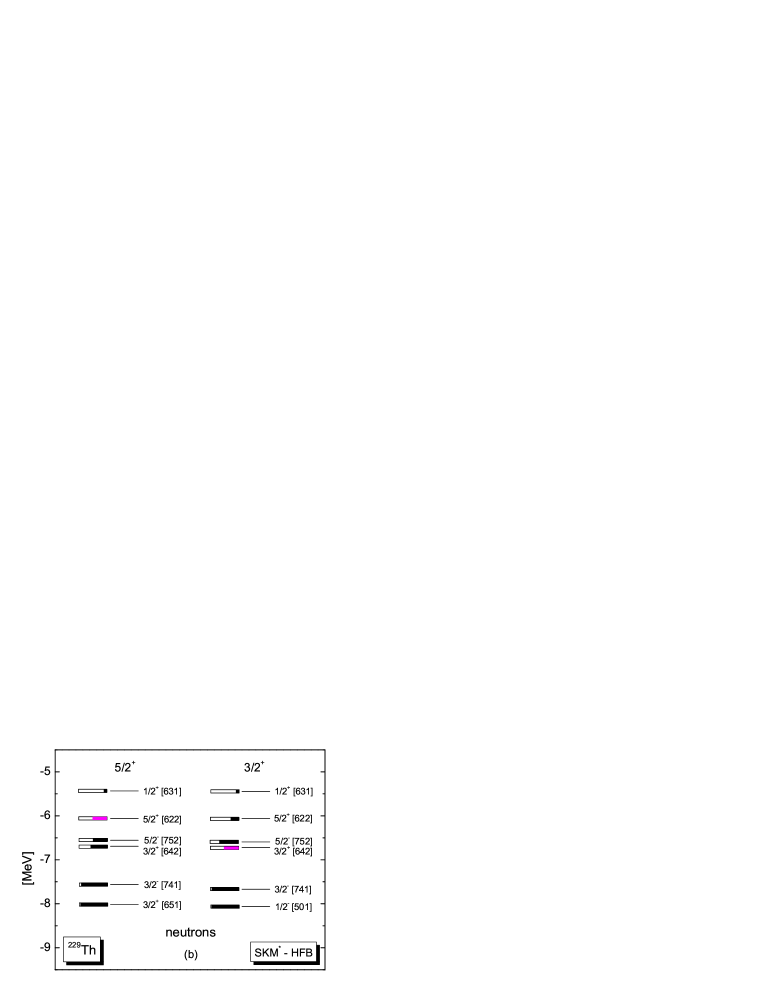
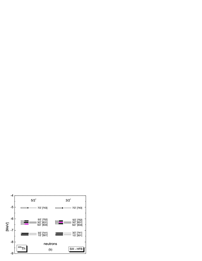
In order to get the experimentally observed parity we perform the variation procedure in the subspace with positive parity. For both energy functionals the Slater determinant with the lowest energy has $K^{\pi}=5/2^{+}$. All energies are summarized in Table 1. The last neutron occupies the level labeled with 5/2⁺[622] in the SkM^∗ and with 5/2⁺[633] in the SIII case. One should keep in mind that the single-particle states are superpositions of Nilsson states and the labeling refers only to the largest component. The states are detailed in Eqs. (53)-(56) below.

The neutron single-particle energies $\epsilon_{\nu}$ and the occupation numbers are displayed in Fig. 3(a) for SkM^∗ and in Fig. 3(a) for SIII. The 5/2^-[752] state which would be occupied in the negative parity case is very close to the 5/2⁺[633] state – for SIII they are almost degenerate.

As can be seen from Table 1, the total HF binding energy agrees with the measured one up to about 9 MeV for the SkM^∗ and up to about 6 MeV for the SIII energy functional. Keeping in mind that no parameters have been adjusted to the specific nucleus considered here it is surprising that these mean-field models can predict the energy with an uncertainty of only about 0.5 %.

Putting two neutrons in the 5/2⁺[622] (for SkM^∗) or 5/2⁺[633] (for SIII) level and one in the 3/2⁺[642] (for SkM^∗) or 3/2⁺[631] (for SIII) level and minimizing the total energy yields an excited HF state that is to be regarded as the intrinsic state of the experimentally observed $K^{\pi}=3/2^{+}$ band. As can be seen in Table 1, the excited states occur at 0.619 MeV for the SkM^∗ and at 0.141 MeV for the SIII density functional. The difference in Coulomb energies $\Delta V_{C}$ amounts to 0.451 MeV for SkM^∗ and to $-0.098$ MeV for SIII. The kinetic energy differences $\Delta T_{p}$ and $\Delta T_{n}$ for protons and neutrons, respectively, dissent even more. These deviations between the two energy functionals reflect the differences in the structure of the intrinsic states as also seen from the difference in the single-particle states discussed above.

V.2 Relativistic mean-field

We also perform a spherical relativistic mean-field calculation with the NL3 parameter set Lalazissis et al. (1997) and find that in the ground state the last neutron occupies a $2g_{9/2}$ orbit. For vanishing deformation the Nilsson state 5/2⁺[633] belongs to the subspace spanned by the spherical $2g_{9/2}$ orbits so that this result is not unreasonable when comparing with the deformed SIII calculation. The leading component for the 3/2⁺ state is for SIII the 3/2⁺[631] orbit (cf. Fig. 3) which for deformation zero belongs to the $1i_{11/2}$ subshell. Therefore we create the excited state with $\Omega^{\pi}=3/2^{+}$ by a particle-hole excitation from the $1i_{11/2}$ to the $2g_{9/2}$ shell so that there are 11 neutrons in the $1i_{11/2}$ and 2 neutrons in the $2g_{9/2}$ shell.

The resulting energies are listed in the last column of Table 1. The total binding energy is similar to the non-relativistic one, but the particle-hole excited state is 2.41 MeV higher. Different from the deformed mean-field the single-particle states of a spherical potential have good total spin $j$ and are $(2j+1)$-fold degenerated with large gaps between them. The single-particle energy difference $\epsilon_{9/2}-\epsilon_{11/2}=2.74$ MeV explains the large excitation energy of the particle-hole pair of 2.41 MeV, which includes the rearrangement energy.

We conclude that a spherical calculation is not appropriate for this particular question. In a recent publication Xiao-tao He and Zhong-zhou Ren (2008) a similar spherical relativistic mean-field calculations comes to results comparable to ours with a Coulomb energy difference of 0.7 MeV. Because of the unphysical properties of a spherical ²²⁹Th we will not commit ourselves to the spherical case any longer but proceed to consider the effects of pairing.

Table 2: Rms-radius and intrinsic quadrupole moments of neutron and proton densities of the ²²⁹Th $5/2^{+}$ ground state calculated with different energy functionals. Differences of these moments between $3/2^{+}$ first excited state and $5/2^{+}$ ground state.

	SkM∗		SIII
$5/2^{+}$	HF	HFB	HF	HFB
$R_{rms}$(neutron)[fm]	5.8789	5.8716	5.8971	5.8923
$R_{rms}$(proton) [fm]	5.7180	5.7078	5.7817	5.7769
$Q_{20}$ (neutron)[fm2]	9.4407	9.2608	9.1990	9.0711
$Q_{20}$ (proton) [fm2]	9.5461	9.3717	9.3542	9.1643
$3/2^{+}-5/2^{+}$
$\Delta R_{rms}$(neutron)[fm]	-0.0040	0.0036	-0.0008	-0.0005
$\Delta R_{rms}$(proton) [fm]	-0.0038	0.0039	0.0000	-0.0005
$\Delta Q_{20}$ (neutron)[fm2]	-0.2427	0.2647	-0.0767	-0.0516
$\Delta Q_{20}$ (proton) [fm2]	-0.1824	0.2756	-0.0339	-0.0495

V.3 Hartree-Fock-Bogoliubov

We include the pairing correlations with the Bogoliubov ansatz (32) and perform a self-consistent HFB calculation based on the SkM^∗ and SIII density-matrix functional. For the SIII case proton and neutron pairing strengths of $V_{0}=-260$ and $-180$ MeV fm³ (for a volume-type contact force) are adjusted to reproduce the total binding energies and the odd-even staggering with the neighboring nuclei. Proton and neutron density matrices and pairing tensors are calculated by including contributions from quasiparticle states up to the cutoff energy of 60 MeV. Calculations are performed by self-consistently blocking the 5/2⁺ and the 3/2⁺ quasiparticle states. In the 5/2⁺ and 3/2⁺ configurations, this yields the average HFB proton and neutron pairing gaps of $\Delta_{p}=2.4$ MeV and $\Delta_{n}=0.65$ MeV, and $\Delta_{p}=2.4$ MeV and $\Delta_{n}=0.68$ MeV, respectively, for the SIII case and slightly larger values for the SkM^∗ case.

The results for the energies are summarized in Table 1 and for the mean-field single-particle energies and the occupation probabilities in Fig. 3(b) and Fig. 3(b). The first to note is that the excitation energy is improving. Its value decreases from 619 keV down to $-46$ keV for SkM^∗ and from $141$ keV down to $-74$ keV for SIII. On the accuracy level one can expect from this model the 5/2⁺ and the 3/2⁺ states are degenerate, like in experiment.

By looking at the occupation numbers displayed in Figs. 3(b) and 3(b) one sees that about 5 single particle levels near the Fermi edge assume fractional occupation numbers significantly different than 0 or 2. In the SIII case (Fig. 3(b)) they are almost identical for the 5/2⁺ and 3/2⁺ states except for the 5/2⁺[633] and 3/2⁺[631] levels that switch their role. For the SkM^∗ case (Fig. 3(b)) the blocked states are energetically further away from each other which causes more deviations in the occupation numbers.

This characteristic pattern of occupation numbers renders the HFB results qualitatively different than the HF ones. Indeed, in the HF case either the 5/2⁺ or the 3/2⁺ orbital has the occupation number equal to 1. Therefore, polarization effects exerted by these two orbitals are able to render different values of observables calculated for the 5/2⁺ and 3/2⁺ states. In the HFB case, occupation numbers of the 5/2⁺ and 3/2⁺ orbitals are close to 1 for both 5/2⁺ and 3/2⁺ configurations. Differences in observables may here only occur due to the fact that the occupation number of the blocked state is exactly equal to 1, while that of the other state is approximately equal to 1, depending on its closeness to the Fermi level.

In the paired case (HFB), we are faced with the situation, where the zero-order approximation renders observables calculated in the 5/2⁺ and 3/2⁺ exactly equal. Indeed, such equality would be the case for the 5/2⁺ and 3/2⁺ orbitals located exactly at the Fermi surface and having exactly the same occupation numbers. Note that values of all observables calculated with the HFB approach depend only on the canonical states and occupation numbers, irrespective of which state has been blocked in obtaining them. Of course, one can obtain different occupation numbers for both orbitals in question when they are energetically split. However, this may contradict the experimental energetic degeneracy of the corresponding configurations. All in all, within a zero-order paired approach, polarization effects of the 5/2⁺ and 3/2⁺ orbitals become exactly averaged out and the anticipated differences in observables can occur only due to first-order corrections.

This fact is perfectly well visible in our results for the Coulomb energy differences shown in Table 1. For the SIII energy functional, only 1 keV remains for $\Delta V_{C}$. This reduces the amplification factor of Eq. (51) to about 100. For SkM^∗ a larger value of $\Delta V_{C}$ of about 300 keV is obtained due to a larger splitting of the corresponding single-particle orbitals. From this one must conclude that pairing correlations result in two states with even more similar charge distributions than in the HF calculation.

V.4 Radii and quadrupole moments

In Table 2 the rms-radii and quadrupole moments (normalized with proton and neutron number, respectively) of the neutron and proton point-densities are given for the ground state and as differences for the excited state. The quadrupole moments of the protons are somewhat larger than for the neutrons. When reoccupying the last neutron the neutron quadrupole moment decreases substantially in the SkM^∗-HF calculation and drags along via the nuclear interaction the quadrupole moment of the protons. At the same time both rms-radii are decreased. A smaller charge radius and smaller charge quadrupole moment are consistent with the increase of the Coulomb energy which explains the large positive $\Delta V_{C}$ in the SkM^∗-HF case. When including pairing the effect goes in the opposite direction for SkM^∗-HFB.

For the SIII functional HF and HFB calculations do not lead to noteworthy changes in the moments when reoccupying the last neutron and thus the Coulomb differences remain also small. This can be anticipated when looking at the single-particle energies of the involved neutron states and the occupation numbers (Fig. 3).

The mean-field single-particle state that corresponds to the blocked HFB state occupied by the unpaired neutron is represented in Nilsson orbits for SkM^∗-HF as

$$\begin{array}[]{llll}\big{|}\,{\frac{5}{2}^{+}}\,\big{>}=&+.509\big{|}\,{622}\,\big{>}&+.467\big{|}\,{642}\,\big{>}&+.266\big{|}\,{862}\,\big{>}\\ &+.402\big{|}\,{633}\,\big{>}&-.397\big{|}\,{613}\,\big{>}&+\cdots\\[4.30554pt] \big{|}\,{\frac{3}{2}^{+}}\,\big{>}=&-.010\big{|}\,{622}\,\big{>}&+.662\big{|}\,{642}\,\big{>}&+.249\big{|}\,{862}\,\big{>}\\ &+.305\big{|}\,{611}\,\big{>}&-.562\big{|}\,{631}\,\big{>}&+\cdots\end{array}$$ (53)

and for SkM^∗-HFB including pairing as

$$\begin{array}[]{llll}\big{|}\,{\frac{5}{2}^{+}}\,\big{>}=&+.504\big{|}\,{622}\,\big{>}&+.487\big{|}\,{642}\,\big{>}&+.248\big{|}\,{862}\,\big{>}\\ &+.418\big{|}\,{633}\,\big{>}&-.383\big{|}\,{613}\,\big{>}&+\cdots\\[4.30554pt] \big{|}\,{\frac{3}{2}^{+}}\,\big{>}=&+.015\big{|}\,{622}\,\big{>}&+.642\big{|}\,{642}\,\big{>}&+.235\big{|}\,{862}\,\big{>}\\ &+.305\big{|}\,{611}\,\big{>}&-.582\big{|}\,{631}\,\big{>}&+\cdots\ .\end{array}$$ (54)

The SIII-HF calculation gives

$$\begin{array}[]{llll}\big{|}\,{\frac{5}{2}^{+}}\,\big{>}=&+.066\big{|}\,{622}\,\big{>}&+.418\big{|}\,{642}\,\big{>}&+.180\big{|}\,{862}\,\big{>}\\ &+.755\big{|}\,{633}\,\big{>}&-.398\big{|}\,{613}\,\big{>}&+\cdots\\[4.30554pt] \big{|}\,{\frac{3}{2}^{+}}\,\big{>}=&+.134\big{|}\,{622}\,\big{>}&+.360\big{|}\,{642}\,\big{>}&+.165\big{|}\,{862}\,\big{>}\\ &+.428\big{|}\,{611}\,\big{>}&-.642\big{|}\,{631}\,\big{>}&+\cdots\end{array}$$ (55)

and the SIII-HFB with pairing

$$\begin{array}[]{llll}\big{|}\,{\frac{5}{2}^{+}}\,\big{>}=&+.024\big{|}\,{622}\,\big{>}&+.423\big{|}\,{642}\,\big{>}&+.159\big{|}\,{862}\,\big{>}\\ &+.775\big{|}\,{633}\,\big{>}&-.367\big{|}\,{613}\,\big{>}&+\cdots\\[4.30554pt] \big{|}\,{\frac{3}{2}^{+}}\,\big{>}=&+.156\big{|}\,{622}\,\big{>}&+.342\big{|}\,{642}\,\big{>}&+.149\big{|}\,{862}\,\big{>}\\ &+.412\big{|}\,{611}\,\big{>}&-.636\big{|}\,{631}\,\big{>}&+\cdots\ .\end{array}$$ (56)

In SIII-HF and SIII-HFB the blocked states exhibit more concentration on the dominant Nilsson orbits $[633]$ and $[631]$. As both have the same nodal structure in $z$-direction ($N_{z}=3$) one expects less difference in the density distribution than in the SkM^∗ case where both states are superpositions of several Nilsson orbits with similar amplitudes. In the SkM^∗ case the leading component of $\big{|}\,{\frac{5}{2}^{+}}\,\big{>}$ is $[622]$ and of $\big{|}\,{\frac{3}{2}^{+}}\,\big{>}$ is $[642]$, which implies a change in nodal structure in $z$-direction. In summary the polarization of the proton distribution due to the reoccupation of the level with the unpaired neutron has less effect in the SIII than in the SkM^∗ case.

In Ref. Hayes et al. (2008) the finite-range microscopic-macroscopic model has been used to study the problem. The authors find small Coulomb energy differences similar to our SIII case. Also the decomposition of the last neutron orbits shows a mixture of several Nilsson orbits resembling more our SIII states than the SkM^∗ states.

We should like to point out that the Nilsson orbit $5/2^{+}[633]$ that is usually used to classify the $K^{\pi}=5/2^{+}$ ground state band Beck et al. (2007); Ruchowska et al. (2006); Barci et al. (2003) does not even contain a single-particle spin $j^{\pi}=5/2^{+}$. Due to positive parity and $\Lambda=|m_{l}|=3$ the orbital angular momenta contained in $5/2^{+}[633]$ are $l=4,6,\dots$. Thus the lowest possible spin in the $5/2^{+}[633]$ Nilsson state is $j^{\pi}=7/2^{+}$. This implies that in a core plus valence-neutron picture the $5/2^{+}[633]$ state needs to be coupled to the excited $J^{\pi}=2^{+}$ state in ²²⁸Th in order to get the ground state spin $J^{\pi}=5/2^{+}$. In the deformed mean-field description the total angular momentum $J^{\pi}=5/2^{+}$ of the nucleus arises from both the $5/2^{+}[633]$ orbital and the underlying deformed ²²⁸Th core.

In Ref. Ruchowska et al. (2006); Gulda et al. (2002) experimental data have been compared with structure calculations for ²²⁹Th that use the quasiparticle-phonon model Soloviev (1976) employing a phenomenological Nilsson mean field and multipole-multipole residual interactions. A very good description of the ²²⁹Th level structure has been achieved by an appropriate fit of the interaction parameters. It has been found that the coupling of the single-quasiparticle degrees of freedom to the collective octupole vibrational state of the ²²⁸Th core is essential to reproduce the parity partner bands observed in experiment. However, as this model is not self-consistent it can not be used for our considerations.

In a fully consistent calculation scheme based on a relativistic density-matrix functional Litvinova and Ring (2006) it has been shown that the coupling to low lying vibrations noticeably improves the description of the single-particle spectrum around the Fermi surface including the ordering of the levels. This model is however programmed only for spherical cases.

One has to realize that the situation is not so simple, valence and core nucleons have to be considered self-consistently and in the next generation of nuclear models, besides the projection of the deformed intrinsic state on total spin and particle number, one also may need to go beyond the mean-field picture by coupling to low-lying core excitations.

V.5 Predictive power and accuracy of observables

In the energy-density functional picture one gives up the explicit knowledge of a microscopic Hamilton operator $H(\boldsymbol{c})$ acting in many-body Hilbert space. Its expectation value is replaced by the energy functional ${\cal E}[\,\mathbf{c},\hat{\rho}\,]$ from which one cannot refer back to the Hamiltonian. It is important to note that one can also not refer back to a many-body state $\big{|}\,{\Psi}\,\big{>}$ that represents an approximation to a true stationary eigenstate of $H(\boldsymbol{c})$. One can of course construct a single Slater determinant with the operators $a^{\dagger}_{\nu}$ which create the occupied states, but this Slater determinant is more an auxiliary object that ensures quantum properties like Pauli principle or uncertainty relation. This Slater determinant misses for example various kinds of typical nuclear correlations that exist in the true eigenstate.

This raises the important question if one has predictive power for other observables than the energy. The believe is that observables which can be calculated from the one-body densities that appear in the energy functionals should be trusted. In our case we calculate Coulomb and kinetic energies, which are given by densities that are included in the set of variational variables of the energy functional ${\cal E}[\,\mathbf{c},\hat{\rho}\,]$ and therefore should be predicted with high accuracy.

Besides these more general considerations there are also concerns about numerical precision. In the SkM^∗ case the Coulomb energy difference $\Delta V_{C}$ = $-0.307$ MeV = $(924.854-925.161)$ MeV is a result of subtracting two big numbers that have been calculated numerically. That means a precision of 10 keV for each of them is desirable. For SIII-HFB, where $\Delta V_{C}$=0.001 MeV, a precision of 0.1 keV is needed. We have checked that we can reach enough numerical precision by sufficient iteration steps.

But there is also the quest for accuracy. Let us for example consider the approximate treatment of the exchange term. Its contribution in HFB-SIII is $-34$ MeV, a 10% error means already 3 MeV uncertainty in $\big{<}\,{V_{C}}\,\big{>}=V^{direct}_{C}+V^{exch}_{C}$. On the other hand one would expect that this is mainly a systematic error that is similar for the two states so that the difference should be less affected, but 1% still means 0.3 MeV error. The actual situation for SIII-HFB is $\Delta V^{direct}_{C}=0.29$ keV and $\Delta V^{exch}_{C}=0.71$ keV which adds up to the $\Delta V_{C}$=0.001 MeV listed in Table 1. In this case the approximate exchange term gives the larger contribution which weakens strongly the confidence in the calculated value of the amplification.

Table 3: Violation of the Hellmann–Feynman theorem $\delta=\alpha_{0}\Bigl{(}\partial E^{tot}(\alpha_{0})/\partial\alpha\Bigr{)}-E^{Coul}(\alpha_{0})$ in HF and HFB calculations with SIII Skyrme functional for ²²⁸Th.

HF	HFB (no cutoff)	HFB (with cutoff)
0.02 keV	0.5 keV	200 keV

As discussed in Sec. II the proper derivation of the equations of motion from an energy functional is crucial for the validity of the Hellmann–Feynman theorem. Without this theorem one would calculate numerically the derivative of the energy with respect to $\alpha$ and create a new source of numerical errors. We tested the validity of the Hellmann–Feynman theorem by comparing to numerical derivatives using a five-point formula. In Table 3 the deviations are listed for the ²²⁸Th ground state of the SIII functional. In the HF calculation the deviation is within the numerical uncertainty induced by the five-point formula. In the HFB calculation one gets also sufficient accuracy when no cutoff in the quasiparticle subspace contributing to the pairing interaction is applied. But the accuracy drops by three orders of magnitude when the density matrices and pairing tensors are calculated by including contributions from quasiparticle states up to the cutoff energy of 60 MeV. The reason is that this truncation does violate the variational structure of the HFB equations J. Dobaczewski, P. Borycki, W. Nazarewicz, and M.V. Stoitsov, to be published . For most observables, this violation induces small effects, and usually can be safely neglected, but it does show up in the very demanding calculation of the Coulomb energy differences.

As discussed before, another accuracy issue is the fact that our model does not contain projection on good total spin and sharp particle number. Also the possibility that configurations could admix that consist of the $K^{\pi}=1^{-}$ band of ²²⁸Th coupled with a single-neutron 5/2^- state cannot be excluded. These questions have to be the task of future investigations.

VI Summary

We have investigated the lowest two states of ²²⁹Th that are almost degenerate in energy. Two very successful energy functionals SkM^∗ and SIII have been employed in a density-matrix functional theory. Hartree-Fock and Hartree-Fock-Bogoliubov calculations have been performed and compared. The result is that for the SkM^∗ functional the difference in Coulomb energy $\Delta V_{C}$ between excited and ground state ranges from $450$ keV without pairing to $-300$ keV when pairing effects are included. On the other hand the SIII-HFB result gives $\Delta V_{C}=1$ keV only. The differences in neutron and proton kinetic energies are of similar size and also quite different for SkM^∗ and SIII.

Altogether, the nuclear models we used predict amplification factors $A=\Delta V_{C}/\omega$, between the drift of the transition frequency $\delta\omega/\omega$ and the drift $\delta\alpha/\alpha$ in the fine structure constant, that have absolute values varying between about $10^{2}$ and $10^{4}$. We have pointed out and discussed the fact that the pairing correlations smooth out polarization effects exerted by the single-particle orbitals. Therefore, such correlations not only dramatically decrease the anticipated amplification factors but also make their determination very uncertain, due to dependence on very detailed properties of the mean-field and pairing effects.

We have also performed spherical calculations and conclude that spherical models should not be consulted as they are too far from reality to provide serious numbers.

As even the sign of the amplification factor is uncertain, much more refined calculations are needed that include coupling to low-lying core excitations and projection on eigenstates with good total angular momentum and particle number. Before being able to provide reasonably trustable numbers how the transition energy varies as function of the fine structure constant $\alpha$ one has to make sure that the model reproduces the three low lying rotational $K^{\pi}=5/2^{+},3/2^{+},5/2^{-}$ bands up to $J\approx 9/2$ and the known electromagnetic transitions within the bands and between them. This would provide more confidence in the quality of the many-body states and their Coulomb energy.

In any case the calculations must treat all nucleons (no inert core) because the whole effect comes from a subtle polarization of the core protons. Furthermore the model has to be of variational type in order to make use of the Hellmann–Feynman theorem. Without that one cannot be sure that the polarization effects caused by the strong interaction are treated consistently with the necessary accuracy. Rough estimates and simple minded models are not sufficient.

The experimental endeavor for measuring the drift of the transition frequency in ²²⁹Th has to be accompanied by substantially improved models on the nuclear theory side and attempts to gain experimental information on the Coulomb energies via radii, quadrupole moments or even form factors. Without a concerted action of experimental and theoretical efforts the goal of improved limits on the temporal drift of fundamental constants cannot be reached.