A nonclassical symbolic theory of working memory, mental computations, and mental set

Abstract

The paper tackles four basic questions associated with human brain as a learning system. How can the brain learn to (1) mentally simulate different external memory aids, (2) perform, in principle, any mental computations using imaginary memory aids, (3) recall the real sensory and motor events and synthesize a combinatorial number of imaginary events, (4) dynamically change its mental set to match a combinatorial number of contexts? We propose a uniform answer to (1)-(4) based on the general postulate that the human neocortex processes symbolic information in a “nonclassical” way. Instead of manipulating symbols in a read/write memory, as the classical symbolic systems do, it manipulates the states of dynamical memory representing different temporary attributes of immovable symbolic structures stored in a long-term memory. The approach is formalized as the concept of E-machine. Intuitively, an E-machine is a system that deals mainly with characteristic functions representing subsets of memory pointers rather than the pointers themselves. This nonclassical symbolic paradigm is Turing universal, and, unlike the classical one, is efficiently implementable in homogeneous neural networks with temporal modulation topologically resembling that of the neocortex.

1 Introduction

Conventional computers process symbolic information by manipulating symbols in a read/write memory – call it a RAM buffer. This classical symbolic computational paradigm encounters serious problems as a metaphor for the symbolic level of information processing in the human brain. It is unlikely that the brain has a counterpart of a conventional RAM buffer. Even if such a buffer existed it would be too small and too slow to allow the brain to efficiently process symbolic information in a traditional way.

Q0. How can the brain produce such cognitive phenomena as working memory, mental computations, and language without a RAM buffer? To tackle this general question, it is helpful to start with the following observations:

1. Working memory. People learn to mentally simulate different external memory aids with the properties of a read/write memory. For example, a highly skilled abacus user learns to compute on an imaginary abacus as efficiently as on the real device [2]. Similarly, an experienced chess player learns to play chess on an imaginary chess board. A computer simulation of a chess board requires a RAM buffer with no less than $n=64$ addresses and $m=13$ symbols – twelve symbols representing chess pieces of two colors and one symbol representing an empty square. This observation raises the question:

Q1. How can a system learn to simulate a RAM buffer?

We show that no learning system that uses a gradient-descent-type or a statistical-optimization-type learning algorithm can learn to simulate even a small RAM buffer with $n=m=2$ (Theorems 1 and 2 of Section 4). Though a RAM buffer is a deterministic system, its behavior is statistically unpredictable in the traditional sense. This means that the human brain cannot rely on the traditional statistical prediction techniques to mentally simulate the behavior of the external world.

2. Turing universality and learning. A person with a good visual memory can be taught to perform, in principle, any mental computation with the use of an imaginary memory aid. Ignoring some theoretically unimportant limitations on the size of the imaginary memory aid, this observation means that the human brain must be treated by a system theorist as a Turing universal learning system. It is interesting to ask:

Q2. What is the simplest architecture of a Turing universal learning system?

This question is directly related to Q1. It is easy to prove that a learning system that cannot answer question Q1 cannot be a Turing universal learning system.

3. Memorization, recollection, and synthesis. People can memorize and recall long sequences of real sensory and motor events. At the same time, they can synthesize a combinatorial number of imaginary events. It is attractive to think that the same learning algorithm can account for all outlined phenomena. We can ask:

Q3. What learning algorithm satisfies the requirements of correct recollection, and combinatorial synthesis?

We argue that a learning algorithm that attempts to do a lot of preprocessing of the learner’s experience before putting this experience in the learner’s LTM cannot answer this question. In contrast, an algorithm that simply memorizes all learner’s “raw” experience, call it a complete memory algorithm (CMA), does not have this limitation (Section 6).

4. Mental set and context. People interpret their inputs differently depending on context. The number of possible contexts explodes exponentially. This leads to a question:

Q4. How can a system with a linearly growing size of knowledge learn to efficiently deal with an exponentially growing number of possible contexts?

This problem of “Attitude and Context” [30] calls into question all traditional approaches to brain modeling and cognitive modeling . The brain cannot have different mental agents [21] for all possible contexts. Accordingly, a consistent answer to Q4 must explain how the brain can dynamically synthesize such agents depending on context.

This paper offers a uniform answer to questions Q1-Q4 based on the assumption that the human neocortex processes symbolic information in a “nonclassical” way. We postulate that, instead of manipulating symbols in a read/write memory, as the classical symbolic systems do, the brain manipulates the states of dynamical memory representing different temporary attributes of immovable symbolic structures stored in a long-term memory. This integrated symbolic-dynamical paradigm is referred to as the concept of E-machine [6, 7, 8]. Answering questions Q1-Q4 provides an insight into the general question Q0.

A complex E-machine (CEM) is a hierarchical associative learning system built from several (many) primitive associative learning systems called primitive E-machines (PEM) (Section 5). A PEM has two main types of states:

(1) The states of encoded long-term memory (LTM) representing symbolic knowledge (software). These states are called G-states, the ‘G’ implying the notion of “synaptic Gain”. (2) The states of different types of dynamical short-term memory (STM) and intermediate-term memory (ITM) accounting for a context-dependent dynamic reconfiguration of the knowledge stored in LTM. These states are called E-states, the ‘E’ implying the notion of “residual Excitation”. The name “E-machine” emphasizes the special importance of the E-states.

We demonstrate some possibilities of the E-machine paradigm by presenting an example of a learning robot with the brain organized as an E-machine. The robot interacts with an external world represented by a keyboard and a screen. The model (implemented as an interactive C++ program) produces the following educational effects:

(1) Working memory. After interacting with an external read/write memory aid the robot learns to mentally simulate this memory aid (creates an imaginary memory aid).

(2) Mental computations. The robot learns to perform computations with the use of the imaginary memory aid.

(3) Mental set and context. The robot interprets its visual input in a combinatorial number of different ways depending on the context created through an auditory input. The rest of the paper consists of the following sections:

2. System (Robot,World) as a cognitive model.

3. The external world as a generalized RAM (GRAM).

4. Limitations of traditional learning systems.

5. The concept of a primitive E-machine (PEM).

6. A PEM can learn to simulate a GRAM.

7. On Turing universality and learning.

8. The effect of a context-dependent mental set.

9. Promising directions of research.

10. Methodological remarks.

2 System (Robot,World) as a cognitive model

The general architecture of the cognitive model used in this paper is shown in Figure 1. The model consists of an external world, W (represented by a keyboard and a screen), and a robot, (D,B), consisting of the sensorimotor devices, D, and the brain, B. From the system-theoretical viewpoint, it is convenient to treat system (W,D,B) as a composition of two subsystems: the external system, (W,D) and the brain B. In this representation, both systems can be viewed as abstract machines, the outputs of (W,D) being the inputs of B, and vice versa. Note that the brain does not know about the external world, W, per se. It knows only about the external system (W,D).

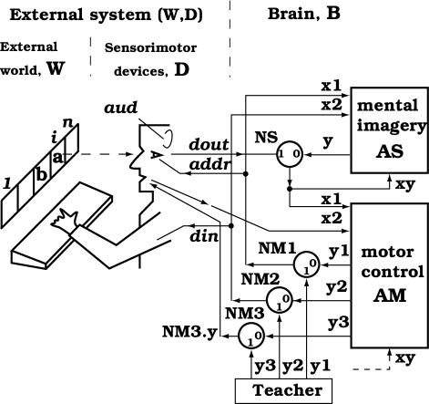
Figure 1: Experimental system

The screen is divided into squares. For simplicity, only one row of squares is shown. For now, we assume that the robot’s eye can see only one square at a time, call it the scanned square – the idea is borrowed from Turing [28]. We also assume that the system has some eye tracking device (not shown), so when the robot depresses a key the character appears in the scanned square.

The external system, (W,D), behaves, essentially, as a RAM. Two motor inputs, $addr$ and $din$, representing the eye position and the typed character, serve, respectively, as the address and data input of the RAM. The sensory (visual) output, $dout$, serves as the data output. There is no control input similar to write-enable input of a RAM. We can say that system (W,D) is in write mode when there is a nonempty motor input, $din$. Otherwise, the system is in read mode. In Section 3.1 we will formalize this verbal description as the concept of a generalized RAM (GRAM).

The diagram depicts a delayed speech feedback, NM3.y $\rightarrow$ AM.x2, and an auditory input, $aud$ (we use “ . ” as the membership operator, that is, AM.x2 denotes input x2 of unit AM). These will be needed in Sections 7 and 8. The robot’s brain is divided into four units:

1. Associative learning system, AS, responsible for sensory memory and mental imagery. The goal of this system is to learn to simulate the external system, (W,D). In this case, (W,D) works as a RAM.

2. Associative learning system, AM, responsible for motor control. The goal of this system is to learn to simulate the teacher.

3. Sensory centers (nuclei), NS, that work as a multiplexer switching between the output from the eye, $dout$, and the output from AS, $AS.y$.

4. Motor centers (nuclei), NM=(NM1,NM2,NM3), that work as a multiplexer switching between the output of the teacher, $T.y=(T.y1,T.y2,T.y3)$, and the output of system AM, $AM.y=(AM.y1,AM.y2,AM.y3)$. We assume that each multiplexer has a select input, $sel$ (not shown), that can be set by the experimenter.

Both systems, AM and AS, are in the, so-called, supervised learning mode. In the course of training, the teacher can produce any desired output of centers NM. The teacher can also switch the output of centers NS ($NS.y$) between the output of system AS ($AS.y$) and the output of the eye, $dout$. When $NS.y=dout$, system (W,D) serves as the teacher for system AS. Both systems, AS and AM, have inputs denoted as $xy$. These inputs deliver the output signals needed for learning. Such inputs are often referred to as desired outputs.

3 The external world as a generalized RAM

3.1 The concept of a generalized RAM (GRAM)

Definition. A generalized RAM (GRAM) is a system $(\textbf{A},\textbf{D},\textbf{M},f)$ (see Figure 2), where

• $\textbf{A}=\{a_{1},...a_{n}\}$ is a set of symbols called address set.

• $\textbf{D}=\{d_{1},...d_{m},\varepsilon\}$ is a set of symbols called data set, where $\varepsilon$ is the empty symbol meaning “no data”.

• $\textbf{M}=\textbf{D}\times...\times\textbf{D}=\textbf{D}^{n}$ is the set of memory states represented as memory arrays $(mem(1),...mem(n))$, where $mem(i)\in\textbf{D}$ is the data stored in the $i-th$ location of GRAM.

• $f:\textbf{A}\times\textbf{D}\times\textbf{M}\rightarrow\textbf{M}\times\textbf{D}$ is a function computing the next memory state and the output data.

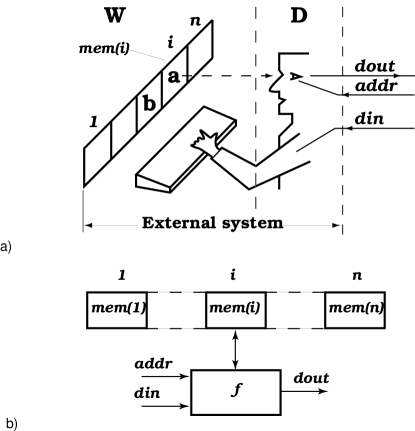
Figure 2: a) The external world appears to the brain as a “RAM buffer”. b) The concept of a generalized RAM (GRAM).

Notation. In what follows, we use a MATLAB-like notation. Array indices start with 1. Symbol “ : ” denotes the range operator. Symbol “$end$” is used as a delimiter in control statements. We add the rightmost parentheses to include a time index. For example, $mem(:)(\nu)$ denotes the value of $m(:)$ at the moment $\nu$. Similarly, $dout(\nu)$ denotes the value of $dout$ at the moment $\nu$.

In discrete time, $\nu$, the work of a GRAM is described by expressions (1) and (2):

(1)     $(mem(:)(\nu+1),dout(\nu))\ =\ f(addr(\nu),din(\nu),m(:)(\nu))$ ;

where function $f$ is

(2)     $if(din==\varepsilon)\ dout=mem(addr);\ else\ \{dout=din;\ mem(addr)=din;\}$ $end$;

The main difference between a GRAM and a conventional RAM is as follows:

1. Both address and data are treated as symbols: that is, only the equal/not equal relationship is defined for the elements of A and D.

2. GRAM is always in write mode when input data is present, $din\neq\varepsilon$. Only if input data is not present, $din=\varepsilon$, is GRAM in read mode. With this approach, we do not need a special control input, e.g., write_enable, to indicate the write or read mode.

One can further extend the notion of GRAM and allow different sets $\textbf{D}^{in}$ and $\textbf{D}^{out}$ of input and output data. What we need is a (not necessarily injective) map $\textbf{D}^{in}\to\textbf{D}^{out}$.

3.2 An experiment with a GRAM

To get used to the notion of GRAM, it is helpful to follow the experiment with a GRAM shown in Figure 3, where $\textbf{A}=\{1,2\}$, and $\textbf{D}=\{a,b,\varepsilon\}$. The three-row table in the upper part of the figure displays the input/output sequence of GRAM as a function of discrete time $\nu=0,1,..9$.

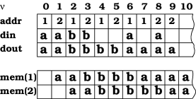
Figure 3: Experiment with a GRAM. $\textbf{A}=\{1,2\}$, $\textbf{D}=\{a,b,\varepsilon\}$. The empty symbol $\varepsilon$ is shown as a blank square.

The $din=\varepsilon$ entries are shown as blank squares. The two-row table in the lower part of the figure displays the contents of the two memory locations, $mem(1),mem(2)$ as functions of $\nu$. The $mem(i)=\varepsilon$ entries are shown as blank squares. For instance, we have
$\nu=0$:
Memory is empty: $mem(:)=(mem(1),mem(2))=(\varepsilon,\varepsilon)$. Input $(addr,din)=(1,a)$ produces output $dout=a$, and writes $a$ into location 1, $mem(1)=a$.
$\nu=3$:
Memory state is: $mem(:)=(b,a)$. Input $(addr,din)=(2,b)$ produces output $dout=b$, and writes $b$ into location 2, $mem(2)=b$.
$\nu=9$:
Memory state is: $mem(:)=(a,a)$. Input $(addr,din)=(2,\varepsilon)$ reads data from location 2, $dout=mem(2)=a$. Memory state does not change.

3.3 Fixed rules and variable rules

Analyzing the three-row input/output table shown in the upper part of Figure 3, we can discover two types of $x\rightarrow y$ rules, where $x=(addr,din)$ and $y=dout$:

1. Rules of the type $(addr,din\neq\varepsilon)\rightarrow dout$, are called fixed rules. In this specific example, the fixed rules are: $(1,a)\rightarrow a$, $(2,a)\rightarrow a$, $(1,b)\rightarrow b$, and $(2,b)\rightarrow b$. There are $m\cdot n=2\cdot 2=4$ such rules. Fixed rules can be easily extracted from the shown input/output sequence by different learning algorithms.

2. Rules of the type $(addr,din=\varepsilon)\rightarrow dout$, are called variable rules. In this example, the variable rules are: $(1,\varepsilon)\rightarrow dout$, and $(2,\varepsilon)\rightarrow dout$. There are $n$ variable rules. The output part, $dout$, of a variable rule depends on the most recently executed fixed rule with the same address. For example, the output of rule $(1,\varepsilon)\rightarrow dout$ at $\nu=7$ is $dout=a$, because the most recently executed fixed rule with $addr=1$ is rule $(1,a)\rightarrow a$ at $\nu=6$. Variable rules cannot be correctly executed by a learning system that does not save information about the most recently executed fixed rules.

It is useful to view fixed rules as a tool for assigning the right parts of variable rules. With this approach, we can say that the meaning or value of an address symbol in a variable rule depends on the most recent assignment. In the discussed example, each address symbol from $\textbf{A}=\{1,2\}$ can be assigned either of two meanings (data values) from $\textbf{D}-\{\varepsilon\}=\{a,b\}$.

4 Limitations of traditional learning systems

Assume that a traditional learning system is used as system AS in Figure 1. It is convenient to redraw the relevant part of Figure 1 as the experimental setup shown in Figure 4, where the external system, (W,D), is replaced by GRAM. Think of input $xy$ as the desired output of the above learning system.

Let $NS.sel=1$, so the GRAM serves as the target system (the teacher) for system AS. We claim that, in this experiment of supervised learning, no traditional learning systems, used as system AS, can learn to simulate the target system with the properties of a GRAM.

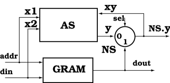
Figure 4: Experimental setup for learning to simulate a GRAM

In what follows we prove this claim for two broad classes of learning systems.

Theorem 1. Let M be a learning system with some statistical (or any other) learning algorithm that learns to predict the output of a target system, T, from the samples of its input/output sequence. Let the maximum length of the samples taken into account not exceed $m$. System M cannot learn to simulate system T with the properties of a GRAM.

Remark. Many learning systems treat a training sequence as a set of input/output pairs. For such systems $m=1$.

Proof. We are going to show that the reaction of a GRAM to the input $(addr,din=\varepsilon)$ is statistically unpredictable. It is sufficient to use a specific example of a GRAM with $\textbf{A}=\{1,2\}$, and $\textbf{D}=\{a,b,\varepsilon\}$ discussed in Section 3.2. A bigger GRAM can always simulate a smaller GRAM, so the result of the theorem will hold for any GRAM with $n\geq 2$. Let us assume that M has learned to predict the behavior of the GRAM. To produce the contradiction, do the following test:

Step 1. Send to the input of M a sequence $x(1),x(2)....x(m+1)$, where $x(1)=(1,a)$, $x(m+1)=(1,\varepsilon)$, and $x(2)=...x(m)=(2,d)$, where $d\in\textbf{D}$. The reaction of the GRAM to this sequence is $dout=a$. Suppose the reaction of M is also $y(m+1)=a$.

Step 2. Send the input sequence which is the same as before, except $x(1)=(1,b)$. By definition, system M predicts its output from the input sequence no longer than $m$, that is, it does not take into account $x(1)$. The reaction of M will again be $y(m+1)=a$. However, the reaction of the GRAM will be $dout=b$. This proves the theorem.

Definition. Let M be a learning system with an input alphabet X. Let $x(1),...x(m1),\dots,$ $x(m2),\dots,x(m+1)$ be an input sequence of the system M, where $1\leq m1<m2\leq m$. We will say that M loses information about the order of input events if there exist $m1$ and $m2$ satisfying the above condition such that for all $z1,z2\in\textbf{X}$, and $z1\neq z2$, the reaction of M is the same for $(x(m1),x(m2))=(z1,z2)$, and $(x(m1),x(m2))=(z2,z1)$.

Theorem 2. No system M that loses information about the order of the input events of the target system can learn to simulate a GRAM.

Proof. Let us use the same GRAM as in Theorem 1. Suppose M satisfies the above definition and nevertheless has learnt to simulate the specified GRAM. To produce the contradiction do the following test:

Step 1. Send to the input of M a sequence $x(1),...x(m1),...x(m2),...x(m+1)$, such that $x(m1)=(1,a)$, $x(m2)=(1,b)$, $x(m+1)=(1,\varepsilon)$, and $x(m2+1)=..x(m)=(2,d)$, where $d\in\textbf{D}$. The reaction of the GRAM to this sequence is $dout=b$. Suppose the reaction of M is $y(m+1)=b$.

Step 2. Send the input sequence $x(1),...x(m1),...x(m2),...x(m+1)$, that is, the same as in step 1, but $x(m1)=(1,b)$, and $x(m2)=(1,a)$. The reaction of the GRAM to this sequence is $dout=a$. However, by definition, the reaction of M to this sequence is the same as before, that is $y(m+1)=b$. This proves the theorem.

Theorems 1 and 2 show that the loss of information at the time of learning leads to principal limitations at the time of decision making. In the case of Theorem 1, system M attempted to predict the output of a GRAM using the samples of the GRAM’s behavior of limited length $\leq m$. In the case of the Theorem 2, M ignored the order of the GRAM’s input events.

5 The concept of a primitive E-machine (PEM)

5.1 An abstract description

A primitive E-machine (PEM) is a system $PEM=(\textbf{X},\textbf{Y},\textbf{E},\textbf{G},f_{y},f_{e},f_{g})$, where

• X and Y are finite sets of symbols called the input and the output set, respectively;

• G is the set of states called the states of encoded (symbolic) long-term memory (LTM) or the G-states. As mentioned before, the letter ‘G’ implies the notion of “synaptic Gain”. The G-states represent the symbolic knowledge (software) of an E-machine.

• E is the set of states, called the states of dynamical short-term memory (STM) and intermediate-term memory (ITM), or the E-states. The letter ‘E’ implies the notion of “residual Excitation”. An E-machine may have several types of E-states representing different temporary attributes (dynamical labels) of the data stored in LTM. The E-states serve as the mechanism for context-dependent dynamic reconfiguration of the knowledge represented by the G-states.

• $f_{y}:\textbf{X}\times\textbf{E}\times\textbf{G}\rightarrow\textbf{Y}$ is a function called, interchangeably, the output procedure, the interpretation procedure, or the decision making procedure.

• $f_{e}:\textbf{X}\times\textbf{E}\times\textbf{G}\rightarrow\textbf{E}$ is a function called, interchangeably, the next E-state procedure, or the dynamic reconfiguration procedure.

• $f_{e}:\textbf{X}\times\textbf{E}\times\textbf{G}\rightarrow\textbf{G}$ is a function called, interchangeably, the next G-state procedure, or the incremental learning algorithm.

Remark. A PEM may have other types of states. For simplicity, these states are not included in the above general description.

The work of a PEM is described in discrete time, $\nu$, as follows:

(1)             $y(\nu)=f_{y}(x(\nu),e(\nu),g(\nu));$

(2)             $e(\nu+1)=f_{e}(x(\nu),e(\nu),g(\nu));$

(3)             $g(\nu+1)=f_{g}(x(\nu),e(\nu),g(\nu));$

with initial states $e(0)$ and $g(0)$,

where $x(\nu)\in\textbf{X}$, $y(\nu)\in\textbf{Y}$, $e(\nu)\in\textbf{E}$, and $g(\nu)\in\textbf{G}$ .

In the next section, we present an explicit example of a PEM. The model is simple enough to be theoretically understandable, but at the same time it is sufficiently complex to produce some nontrivial cognitive phenomena. This PEM will be used as system AS and system AM of Figure 1.

5.2 An example of a primitive E-machine

Figure 5 illustrates the architecture of a simple PEM. The interpretation procedure $f_{y}$ is divided into four elementary procedures: DECODING, MODULATION, CHOICE, and ENCODING.

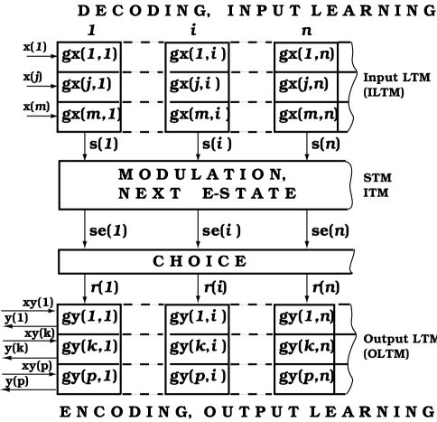
Figure 5: Example of a primitive E-machine

The model uses a single E-state array, $e(i)$. The next E-state procedure, $f_{e}$, is similar, in this example, to the fast-charging-slow-discharging of a capacitor. The model employs a universal learning algorithm, $f_{g}$, that simply tape-records input/output associations in the LTM. The recorded association gets an elevated level of residual excitation to produce an effect of recency. This is described as the addition to the next E-state procedure.

Variables:

• $\nu\in\{0,1,...\}$ is a discrete time (the cycle number).

• $x(:)\doteq x(1),..x(m)$ is the input vector with $m$ components. In this example, each component is treated as a symbol. That is, only the equal/not equal relationship is defined. As before, we use a special empty symbol, $\varepsilon$, to indicate “no data”.

• $wx(:)\doteq wx(1),..wx(m)$, where $wx(j)>0$ $(j=1,..m)$ is the vector describing the weights of input symbols.

• $gx(:,i)\doteq gx(1,i),..gx(m,i)$ is the vector stored in the $i$-th location of the Input LTM (ILTM), where $i\in\{1,...n\}$.

• $s(:)\doteq(s(1),..s(n))$ is a similarity array. In general, $s(i)$ is a nonnegative real number representing a similarity between $x(:)$ and $gx(:,i)$. In this example, we use a very simple criterion of similarity – the number of matching non-empty symbols. Accordingly $s(i)\in\{0,1,...m\}$.

• $e(:)\doteq(e(1),..e(n))$ is an E-state array. Variable $e(i)$ is a nonnegative real number that represents the level of residual excitation associated with the $i$-th location of the LTM. In this example, we use a single E-state array. In more complex models, several E-state arrays, $e1(:)$, $e2(:)$,…, with different dynamic properties can be used.

• $se(:)\doteq(se(1),..se(n))$ is modulated or biased similarity array. In general, $se(i)$ is an element of a real array that describes the similarity affected by the residual excitation.

• $r(:)\doteq(r(1),..r(n))$ is a retrieval array. In general, $r(i)$ is an element of a real array that represents the level of activation of the $i$-th location of OLTM. In this model, we use a random winner-take-all choice, so only one component of this array, $r(iwin)$, corresponding to the winner, $iwin$, is not equal to zero. Formally, in this example we need only the variable $iwin$. The $r$-array is introduced for the sake of completeness. It does not appear in the following equations. This array is needed in more complex models of primitive E-machines that employ more complex encoding procedures.

• $gy(:,i)=gy(1,i),..gy(p,i)$ is the vector stored in the $i$-th location of the Output LTM (OLTM). In this model, components of $gy(:,i)$ are treated as symbols.

• $y(:)=y(1),...y(p)$ is the output vector retrieved from OLTM. In this model the output is read from the winner location of OLTM. Components of $y(:)$ are treated as symbols.

• $xy(:)$ is the input to the OLTM used for writing output data in this memory.

• $wptr$ and $wen$ are the auxiliary variables used to describe the tape-recording learning algorithm. They serve as the write_pointer and the write_enable, respectively.

Parameters:

• $a<0.5$ is a parameter that determines the modulating effect of $e(i)$ on $s(i)$ that produces biassed similarity $se(i)$.

• $c<1.0$ is a parameter that determines the rate of decay of $e(i)$. The time constant of decay is $\tau=1/(1-c)$, so $c=1-1/\tau$.

• $m$ is the number of components in the input vector $x(:)$.

• $n$ is the number of locations in the ILTM and OLTM. It is the size of all arrays with index $i$. Namely, $s(i)$,$se(i)$,$e(i)$, $gx(:,i)$, and $gy(:,i)$.

• $p$ is the number of components in the output vector $y(:)$.

Remark. In the experiments discussed in this paper, weights, $wx(:)$, will be treated as parameters. In more complex experiments the pair $(x,wx)$ can be treated as an input.

Procedures:

DECODING (computing similarity):

$for$ $i=1:n$    (this for is applied to expressions (1), (2), and (5))

(1)             $s(i)=\sum_{j=1}^{m}{wx(j)\cdot T(x(j)=gx(j,i)\neq\varepsilon)}$

where,  $T(z)=1$, if $z=true$, else $T(z)=0$

MODULATION (computing biased similarity):

(2)             $se(i)=s(i)\cdot(1+a\cdot e(i))$

CHOICE (randomly selecting a winner):

(3)             $iwin\ :\in\ \{i:se(i)=max(se)>0\}\ \doteq\ \textbf{MSET}$

where $:\in$ denotes the operation of the random equally probable choice of an element from a set.

ENCODING (retrieving data from OLTM):

(4)             $y(:)=gy(:\ ,iwin)$

NEXT E-STATE PROCEDURE (dynamic reconfiguration):

(5)             $if\ (s(i)>e(i))\ e(i)(\nu+1)=s(i)\ ;\ else\ e(i)(\nu+1)=c\cdot e(i);$  $end$

where, $e(i)(\nu+1)$ is the value of $e(i)$ at the next moment $\nu+1$. For simplicity, we do not write $\nu$ in the current values of the variables. That is, $e(i)$ is the same as $e(i)(\nu)$, $s(i)$ is the same as $s(i)(\nu)$, etc.

NEXT G-STATE PROCEDURE (learning)

(6)             $if(wen==1)\ gx(:,wptr)(\nu+1)=x(:);\ gy(:,wptr)=xy(:)$;
.                                           $wptr(\nu+1)=wptr+1;$ $end$

Remark. Expression (6) tape-records input and output vectors in the ILTM and OLTM, respectively, when recording is enabled, $wen=1$. For simplicity, in this model, we assume that the weights of input symbols, $wx(:)$, do not affect recording. We will always have $wx(j)\geq 1.0$.

ADDITION to the NEXT E-STATE PROCEDURE (the recorded location of LTM,
$i=wptr$, gets initial residual excitation)

(7)             $if(wen==1)\ e(wptr)(\nu+1)=s(wptr)=\sum_{j=1}^{m}{wx(j)\cdot T(x(j)\neq\varepsilon)};$ $end$

Remark. The truth function $T(z)$ is defined in expression (1). Expression (7) adds residual excitation to the location of ILTM with $i=wptr$, – the location in which data was just recorded. This happens only if recording is enabled, $wen=1$. The level of added residual excitation, $e(wptr)$, is equal to the one that would be produced if the input vector $x(:)$ were already recorded in this location of ILTM, that is, as if $gx(:,wptr)=x(:)$. This trick allows one to avoid introducing intermediate steps in the $\nu-th$ cycle.

System of references. The model described above will be referred to as Model (5.2) or PEM (5.2), meaning the model (PEM) described in Section 5.2. Similarly, expression (5.2.6) will mean expression (6) of Section 5.2, etc.

5.3 On neural implementation of primitive E-machines

It is helpful to have an intuitive link between E-machines and neural networks. Such a link provides a source of neurobiological heuristic considerations for the design of the models of E-machines and the source of psychological heuristic considerations for the design of the corresponding class of neural models. Figure 6 shows the general architecture of a homogeneous neural network corresponding to a PEM. The architecture was discussed in [7, 9].

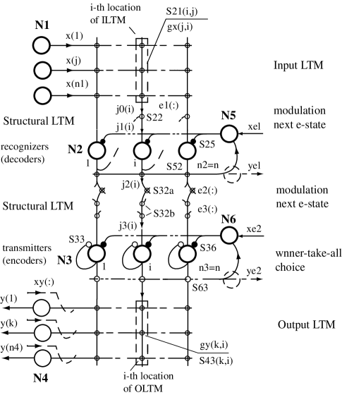
Figure 6: An example of a neural implementation of a primitive E-machine

Large circles with incoming and outgoing lines represent centers – elements that are assigned certain coordinates in the network. A center with incoming and outgoing lines can be interpreted as a neuron with its dendrites and axons, respectively, or a network functionally equivalent to a “large neuron”. Small circles represent couplings – the elements whose position in the network is described by a pair of centers communicating through this coupling. A coupling can be interpreted as a synapse or a circuit functionally equivalent to a “large synapse”. The white and the black small circles represent excitatory and inhibitory synapses, respectively. In what follows we use the terms neuron and synapse instead of the terms center and coupling, respectively .

Figure 6 displays six sets of neurons (N1, N2, N3, N4, N5, and N6) and 10 sets of synapses (S21, S22, S25, S52, S32a, S32b, S33, S36, S63, S43).

Nj(i) is the $i$-th neuron from the $j$-th set. Skja(n,m) is the synapse between neurons Nj(m) and Nk(n), where ’a’ is an additional index describing the type of synapse (in case there are several different types of synapses between the sets of neurons Nj and Nk). The ’:’ substituted for an index indicates the whole subset of elements (variables) corresponding to the entire set of values of this index. S21(i,:)$\doteq$(S21(i,1),…S21(i,n1)). S21(:,:) is the same as S21, etc.

The diagram depicts three types of synapses with E-states: $e1(:)$,$e2(:)$, and $e3(:)$, serving different purposes. $e2(:)$ is similar to the $e(:)$ of Model 5.2; e1(:) describes the effect of lateral modulation that allows the network to decode temporal sequences; e3(:) describes spreading residual excitation producing the effect of broad temporal context. Note. This neural network corresponds to a PEM more complex than Model (5.2) [7, 9].

The Input LTM and the Output LTM are implemented, respectively, as the input, and output synaptic matrices, $S21(:,:)$ and $S4(:,:)$. The network also has some intermediate synaptic memory called Structural LTM (SLTM). This memory corresponds to modifiable connections among neuron decoders, N2, and neuron encoders, N3.

Layer N3 implements a winner-take-all (WTA) choice. The layer has local excitatory feedbacks, S33, and a global inhibitory feedback via neuron N6 – the, so-called, inhibit-everyone-and-excite-itself principle. The WTA choice could also be implemented by using inhibitory synapses S33(i2,i1) with gains $\geq 1.0$ for all synapses except those with $i2=i1$ – the, so-called, inhibit-everyone-but-itself principle.

Layer N2 has an inhibitory feedback with the gain less than unity to provide contrasting. Both layers, N2 and N3, have inhibitory inputs xe1, and xe2. The diagram also depicts some outputs ye1, ye2 carrying information about the global levels of activation of the corresponding layers. One can invent different functional models of primitive E-machines corresponding to the network of Figure 6. However, an attempt to discuss this interesting topic in more detail would take us too far from the goal of this paper.

Remarks:

1. To implement very large ILTM and OLTM one needs intermediate neurons to increase the fan-out of input neurons N1, and the fan-in of output neurons N4. Some ideas inspired by the organization of the cerebellum were discussed in [7].

2. The concept of E-machine supports the notion that the E-states (the states of dynamic STM and ITM) are associated with the properties of individual neurons and synapses. There is an interesting possibility to formally connect the dynamics of the phenomenological E-states with the statistical conformational dynamics of ensembles of membrane proteins treated as Markov systems [11].

3. Some neural network researchers strongly oppose the notion of symbols in the brain. We argue that this anti-symbolic bias is counterproductive. There is an interesting possibility to represent symbols in ILTM and OLTM as sparse quasi-orthogonal synaptic vectors (see items 7, 8, and 9 in Section 9).

4. It is challenging to try to find neurobiological mechanisms that could provide an implementation of learning algorithms functionally close to the complete memory algorithm used in Model (5.2). Such mechanisms may exist, taking into account the principle limitations of the traditional learning algorithms demonstrated in Section 4.

6 A PEM can learn to simulate a GRAM

Theorem 3. The PEM described in Section 5.2 used as system AS in the experimental setup of Figure 4 can learn to simulate a GRAM from a sample of the GRAM’s behavior of the length $\geq n\cdot m$.

Proof. First of all, we need to specify the parameters of the PEM (5.2) and the conditions of the experiments.

System AS is organized as Model (5.2) with parameters $AS.m=2$; $AS.p=1$;
$AS.wx(1)=AS.wx(2)=1.0$. We assume that $AS.n$ is as big as needed to record all training data.

Remark. We add the name AS to the names of parameters of Model (5.2), to avoid confusion with the parameters of the GRAM. The names $m$ and $n$ refer to the parameters of GRAM.

The experiment is divided into two parts: training, and examination. Training starts at $\nu=0$ and lasts until $\nu=\nu 1-1$. During training $NS.sel=1$, that is, $AS.xy=dout$. Writing to LTM is enabled, $AS.wen(\nu)=1$. At the beginning of training, the write pointer is in the initial position, $AS.wptr(0)=1$, and the LTM is empty, $AS.gx=AS.gy=\varepsilon$, and residual excitation is set to zero, $AS.e(:)=0$. We assume that during training each fixed rule of the GRAM is recorded at least once in the LTM. Since the number of such rules is $n\cdot m$, we need $\nu 1\geq n\cdot m$.

Examination starts at $\nu=\nu 1$ and lasts as long as needed. During examination $NS.sel=0$, that is, $AS.xy=AS.y$. For simplicity we assume that writing to LTM is disabled, $wen(\nu)=0$. Note. Writing could be enabled during examination. This would make no difference as far as Theorem 3 is concerned.

We begin with a verbal explanation of the effect of working memory . The effect is produced by decaying residual excitation, $e(i)$, associated with locations of LTM.

Let the $i$-th location of the LTM (ILTM and OLTM) contain the record of the following fixed rule: $gx(1,i)=a,gx(2,i)=d,gy(1,i)=d$, where $a\in\textbf{A}$ and $d\in\textbf{D}-\{\varepsilon\}$. The residual excitation $e(i)$ associated with this location can reach the maximum possible level, $emax=2$, in two situations:

1. At the next moment after the rule was recorded in the $i$-th location. This is the result of expression (7) from Section (5.2) (expression (5.2.7)) which sets residual excitation at the moment of recording.

2. If the rule is already recorded and input is $x(1)(\nu)=a$, and $x(2)(\nu)=d$. In this case, $e(i)(\nu+1)=2$ is a result of expressions (5.2.1) and (5.2.5).

Once the $e(i)=emax$ is set, we can say that the rule $(a,d,d)$ is placed in working memory. The reason for this statement is that, if we send input $x(1)=a$ $x(2)=\varepsilon$ the output $y(1)$ will be retrieved from one of the locations of LTM with the highest level of residual excitation among locations for which $gx(1,i)=a$. Locations for which $gx(1,i)\neq a$ will have $s(i)=0$ due to expression (5.2.1). Accordingly, due to expression (5.2.2), for these locations $se(i)=0$ independently of the level of residual excitation. This effect of executing the most recent rule placed in working memory will last until $e(i)$ decays below a certain level, $eloss$. For this model $eloss=1$ and the modulating coefficient, $a$, in expression (5.2.2) must be less than $1/emax=.5$. Due to expression (5.2.5), the time of decay of $e(i)$ from $emax$ to $eloss$ is

(1)     $tmax\ =\ \ln(eloss/emax)/\ln(c)=-\ln(emax/eloss)\cdot\ln(1-1/\tau)>\ \tau\cdot ln(emax/eloss)$

where $c=1-1/\tau$, and, for this model, $emax/eloss=2$. We can transform this qualitative explanation into a rigorous proof by verifying the following statements:

S1. At $\nu=\nu 1$ (the beginning of examination) LTM of AS contains at least once any fixed rule $(addr,din,dout)\in\textbf{A}\times\textbf{D}^{\prime}\times\textbf{D}^{\prime}$, where $\textbf{D}^{\prime}=\textbf{D}-\{\varepsilon\}$. Formally,

(2)     $\forall(addr,din,dout)\in\textbf{A}\times\textbf{D}^{\prime}\times\textbf{D}^{\prime}\ \exists i(gx(1,i),gx(2,i),gy(1,i))=(addr,din,dout))$

This statement follows from expression (5.2.6) and the definition of the experiment of training. During training $wen=1$, so the training sequence containing all fixed rules is tape-recorded in LTM.

S2. At $\nu=\nu 1$ all location of LTM containing fixed rules have $e(i)>0$ due to expression (5.2.7). Let $tmax>\nu 2-\nu 0$. From expression (1) we find that to guarantee that $e(i)=emax=2$ will not decay below $eloss$ during the entire experiment of training and examination it is sufficient to have $tmax\geq\nu 2-\nu 0$. This condition is satisfied if

(3)     $\tau\geq\ \tau min\doteq(\nu 2-\nu 0)/ln(eloss/emax)\ =\ (\nu 2-\nu 0)/ln2$

S3. Suppose in the course of examination we test AS only in the read mode. That is, we send only inputs $addr,din$ with $din=\varepsilon$. Then $y(1)$ will be retrieved from a location $ird$ for which $gx(1,ird)=addr$ and $e(ird)$ has the highest level among all locations with $gx(1,i)=addr$. If $\tau\geq\tau min$, it is guarantied that $e(ird)>eloss$, so $y(1)$ will be retrieved from the location in which a certain data, $din\neq\varepsilon$ was recorded most recently and, therefore, $y(1)=din$. This is exactly how GRAM would react to this input.

S4. Let $\nu w$ and $\nu r$, where $\nu r>\nu w$ be some “write” and “read” moments in the course of examination, such that $x(1)(\nu w)=addr$, $x(2)(\nu w)=din\neq\varepsilon$ and $x(1)(\nu r)=addr$, $x(2)(\nu r)=\varepsilon$. Let there be no other input between $\nu w$ and $\nu r$ with the same $x(1)$ and different $x(2)\neq\varepsilon$. Due to expression (5.2.5) $e(i)(\nu w+1)=emax=2$ for all $i\in\{i:gx(1,i)=addr,gx(2,i)=din\}$. Accordingly, due to what was said in S3, $y(1)(\nu r)=din$. Again, AS reacts exactly as GRAM.

This proves the theorem, since all other possible cases of “writing to working memory” and reading from this memory can be reduced to S3 and S4.

Remark. Why, in this model should the data loss level, $eloss$, be set at 1? The reason for that is that the residual excitation $e(i)=1$ can be created in a wrong location by $x(2)=din\neq\varepsilon$. Accordingly, only the residual excitation higher than 1 can be relied upon. The $e(i)>1$ can only be the result of decay from level emax=2. The latter level can be set only by the input $x(1)=addr$, $x(2)=din\neq\varepsilon$. This input corresponds to writing non-empty data, $din\neq\varepsilon$, to an address, $addr$, of GRAM.

7 On Turing universality and learning

We have already shown that system AS of Figure 1, organized as PEM (5.2), can learn to simulate a GRAM with $n$ locations and $m$ data symbols in $n\cdot m$ steps. To make the brain, $B=(NS,NM,AS,AM)$, a Turing-universal learning system, we need a system AM capable of learning to simulate the finite-state part of a Turing machine (5.2).

Because of the delayed speech feedback, NM3.y $\rightarrow$ AM.x2, it is sufficient for AM to be a learning system universal with respect to the class of combinatorial machines. The PEM (5.2) satisfies this requirement.

Theorem 4. System AM, organized as PEM (5.2), can be taught, in the experimental setup of Figure 1, to simulate, in principle, any combinatorial machine with 2-inputs and 3-outputs. The above statement holds for any $m\geq 1$ and $p\geq 1$.

Proof. Let $AM.m=2$, $AM.p=3$, $AM.wx(:)=1.0$, $AM.a=0$. The latter means that modulation is turned off, and, according to Expression (5.2.2), $AM.se(i)=AM.s(i)$.
As in Section 6, we divide the experiment into two stages: training and examination.

At the stage of training $NM.sel=NS.sel=1$. The input vector, is coming from system (W,D), that is, $AM.x(1)=dout$, and the output vector is coming from the teacher, that is, $AM.xy(:)=NM.y(:)=T.y(:)$. Training starts at $\nu=0$ and ends at $\nu=\nu 1-1$. At the beginning of training the LTM is empty, $AM.(gx,gy)(0)=0$, and the write pointer is in the initial position, $AM.wptr(0)=1$. Writing is enabled during training, $AM.wen(\nu)=1$ for $\nu=0,...\nu 1-1$.

At the stage of examination, $\nu\geq\nu 1$, writing is disabled, $AM.wen(\nu)=0$, and $NM.sel(\nu)=0$, that is the output, $NM.y(:)$ is produced by system AM, $NM.y(:)=AM.y(:)$. The teacher controls select signal $NS.sel$ and can switch it between the external system, (W,D), and the imaginary external system, the role of which is played by system AS.

Since, at the stage of training, the teacher controls all motor signals $NM.y(:)$, any set of productions $AM.(gx(1,i),gx(2,i))\rightarrow AM.(gy(1,i),gy(2,i),gy(3,i))$ can be formed in the LTM of system AM. It is easy to verify that these productions will be correctly interpreted (executed) by Expressions (5.2.1),(5.2.2),(5.2.3), and (5.2.4). Expression (5.2.2) is reduced to $se(i)=s(i)$ since $a=0$, and, consequently, Expressions (5.2.5) and (5.2.7) have no effect. This completes the proof.

Remarks:

1. To transform the system of Figure 1 into a working model one needs to take care of the synchronization of units (W,D),NS,NM,AS, and AM. These technical problems are of no significance for the purpose of this paper. The model was actually implemented as an interactive C++ program for the MS Windows called EROBOT.

2. The model has an interesting psychological interpretation. It suggests that the Turing universality of human thinking is a result of mental interaction of the motor system, AM, that forms $Sensory,Motor\rightarrow Motor$ ($SM\rightarrow M$) associations, and the sensory system, AS, that forms $MS\rightarrow S$ associations. The symbols M and S in the left parts of the associations suggest motor and sensory feedbacks. Using the terminology borrowed from [3], system AM can be called the central executive. It has a speech feedback that produces the effect of the internal states (the states of mind) of the simulated Turing machine. The robot needs to talk to itself to be able to perform, in principle, arbitrarily complex computations.

8 The effect of a context-dependent mental set

So far we have demonstrated the importance of the E-states in the sensory system AS. The introduction of the E-states in the motor system AM leads to an interesting effect of context-dependent mental set. We are going to show that the PEM (5.2) used as AM can acquire the knowledge needed to simulate $N=2^{2^{m}}$ $m$-input Boolean functions during only $n=2^{m+1}$ steps of training. The effect is achieved due to a context-dependent dynamic reconfiguration of this limited knowledge at the time of decision making. Let $m=10$. Then $n=2048$ and $N=2^{1024}$. In the shown case, k=2, n=8, and N=16.

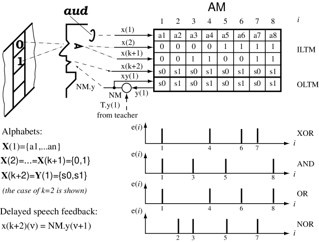
Figure 7: Experimental setup for demonstrating the effect of context-dependent mental set.

Let us modify the experimental system of Figure 1 as shown in Figure 7. We connect the auditory channel, $aud$, and allow the robot to see several squares at a time. In the discussed experiment, the robot does not need to type on the keyboard. It expresses its reactions via the speech channel. We removed system AS and centers NS. These units are not needed in the discussed experiment.

Let AM be described as PEM (5.2) with $m=k+2$, and $p=1$. In Figure 7, $k=2$. The table displays the contents of LTM after $n=2^{k+1}=2^{3}=8$ steps of training. The upper part of the table shows the contents of ILTM, $gx(1:k+2,1:n)=gx(1:4,1:8)$. The lower part shows the contents of OLTM, $gy(1,1:n)=gy(1:8)$. Each association, $gx(:,i)\rightarrow gy(1,i)$, has $k+2=4$ input symbols and one output symbol. To understand the structure of an association consider the association at $i=3$. The upper symbol $gx(1,1)=a3$ represents an auditory name assigned to this association. The name is taken from the set (alphabet) of auditory names $\textbf{X}(1)=\{a1,...a8\}$.

Symbols $gx(2:3,3)=(0,1)$ represent the visual input read from the screen. The symbols are taken from the visual alphabets $\textbf{X}(2)=..\textbf{X}(3)=\{0,1\}$ In this experiment, the robot can see $k=2$ visual symbols simultaneously through inputs $x(2:3)$. At the moment shown, the robot sees symbols $x(2:3)=(0,1)$.

The output symbol, $gy(1,3)=s0$ represents the motor speech symbol corresponding to the reaction $0$ – the robot simulates a Boolean function with the input read from the screen, and the output represented as a motor speech symbol. The motor speech symbols are taken from the alphabet $\textbf{Y}(1)=\{s0,s1\}$. The diagram depicts a delayed proprioceptive speech feedback, $x(k+2)(\nu)=NM.y(:)(\nu+1)$. At $i=3$, the corresponding proprioceptive symbol is stored as $gx(k+2,3)=s0$. The role of the proprioceptive speech feedback is explained later.

In what follows we give a verbal explanation of the work of the model. The explanation can be transformed into a rigorous proof in the same way it was done in Section 6. As before, the experiment is divided into two stages: training and examination. We assume that the model has a RESET button that allows the experimenter to set $e(:)=0$, and a GO/STOP button to start and stop execution. We also assume that the speech feedback can be turned ON and OFF. If it is OFF, $x(k+2)=\varepsilon$. We start with the case when the feedback is OFF, so for a while we disregard $gx(k+2,i)$ and $x(k+2)$.

At the beginning of training, LTM is empty, $gx,gy=\varepsilon$, and the write pointer is in the initial position, $wptr=1$. During training, writing is enabled, $wen=1$, and the teacher creates associations corresponding to all productions participating in all $k$-input Boolean functions. The number of such productions, and the minimum length of training, is $n=2\cdot 2^{k}$. In the shown case, $n=2\cdot 2^{2}=8$. Each production is given a unique auditory name from $\{a1,..an\}$.

At the stage of examination, writing is disabled, $wen=0$. Using auditory input x(1), the experimenter pre-tunes (pre-activates) a set of associations corresponding to a given Boolean function by sending the auditory names of these associations via input $x(1)$. Let all $wx(j)=1.0$ for $j=2,..k+1$, and $wx(1)>k+1$. In this case the maximum level of residual excitation, $e(i)$, created via the auditory channel will be bigger than the maximum level of excitation created via all other channels. Since the time of decay of residual excitation can be made arbitrarily big, any number of productions can be put into working memory (cf Section 6). While residual excitation of the selected subset of associations stays above the loss level, $eloss$, the robot will execute the pre-tuned Boolean function. For the discussed model $eloss=k$.

We can now explain the idea of the speech feedback. Suppose each input cycle is divided into two steps. At the first step, the robot executes the association as if there is no feedback. At the second step, proprioceptive input $x(k+2)$ arrives and increases the level of residual excitation of the executed association. Then the feedback is interrupted, and the next cycle starts. And so on. This refresh mechanism will produce the effect of a self-supporting mental set. (One needs to slightly modify the learning algorithm and the training procedure to correctly record the proprioceptive symbols into $gx(k+2,wptr)$.

9 Promising directions of research

There are many interesting problems and possibilities associated with the development, exploration, and understanding of the symbolic-dynamical computational paradigm represented by E-machines [7]. These include:

1. Decoding temporal sequences. Adding lateral pre-tuning to the next E-state procedure addresses this problem. The corresponding PEM can learn to simulate, in principle, any output independent finite memory machine. Introducing a delayed feedback in the above PEM leads to a system capable of learning to simulate any output dependent finite memory machine.

2. Waiting associations. One can add an E-state creating an effect of waiting association. In this way one can produce an effect of a finite stack without using a RAM buffer, and simulate context-free grammars with limited memory. This allows one to get an effect of calling and returning from subroutines.

3. Broad temporal context. This effect can be produced by adding different types of “spreading” E-states. Changing the time constants and the radii of spread of such states leads to the effects of mental set significantly more complex than that discussed in Section 8.

4. Active scanning of associative memory. People can answer the questions about what happened after or before a certain event. This effect can be achieved by first creating an E-state profile that activates the information about the mentioned event, and then actively shifting this profile in the time-wise or counter-time-wise direction. This can be done by introducing additional control inputs in a PEM.

5. Inhibiting data with given features. One does not have to think about the E-states as “excitations” or “activations”. One can imagine the E-states producing inhibiting, pre-inhibiting, pre-activating, post-activating, etc. effects. In fact, any functions over sets of data stored in the LTM that assign some dynamic labels to the subsets of data can be thought of as different kinds of E-states. For example, one can imagine a situation in which one first creates an E-state activating a set of data (by addressing this data by content) and then temporarily inhibits the selected set of data by sending some inhibiting control input. The brain has many different neurotransmitters and receptors that may justify different hypotheses about the possible types of such control inputs. From the viewpoint of this paper, the important thing is that different hypotheses of this type can be efficiently expressed in terms of the E-machine formalism.

6. Connecting the dynamics of E-states with the statistical conformational dynamics of ensembles of membrane proteins. There is an interesting possibility of connecting some E-states with the statistical conformational dynamics of the ensembles of membrane proteins treated as probabilistic molecular machines (PMM) [10, 11]. A PMM is a Markov system with the transitional probabilities depending on macroscopic inputs such as membrane potentials, and concentrations of neurotransmitters [15, 24]. With this approach, an ensemble of PMMs (EPMM) becomes a statistical mixed signal computer in which the E-states can be interpreted as the occupation numbers of different microscopic states of PMMs. The formalism is a natural system theoretical extension of the classical Hodgkin and Huxley (HH) theory [16], and works well for the generation of spikes [11]. Validating this approach for representing the dynamics of short-term and intermediate-term memories would justify postulating quite complex next E-state procedures.

Remark. There can be many different hypotheses as to how the E-states of different types could be implemented at the cellular level [19, 22]. Translating such neurobiological hypotheses into next E-state procedures gives one a mathematical tool for exploring psychological implications of these hypotheses.

7. Effects of drugs on higher mental functions. As shown in Section 8, changing dynamical E-states changes the symbolic personality of an E-machine. Accordingly, the E-machine formalism gives one a tool for expressing a broad range of ideas about how different drugs could affect higher mental functions by affecting the E-states.

8. From signals to symbols and vice versa. The most likely candidate for the E-machine paradigm is the neocortex. To make this paradigm practically implementable at the higher level, the lower levels of the brain must be able to convert sensory signals into sensory symbols, and motor symbols into motor signals. One of the possibilities is that the signal-to-symbol conversion is done by different feature detectors. Each detector would have a fixed sparse ID serving as a unique pointer to this detector. The sets of such IDs would form primary sensory alphabets. Similarly, the units generating primary motor features would have sparse IDs forming primary motor alphabets. With this approach, the higher association areas of the neocortex could deal mostly with symbols.

9. Sparse recoding in a hierarchical structure of associative memory. As mentioned before, a complex E-machine (CEM) is a hierarchical associative learning system built from several PEMs. The concept of sparse IDs can be extended to allow the PEMs of higher levels to store data in terms of sparse-recoded references to the data stored in the PEMs of lower levels. This would naturally produce different effects of data compression and chunking [1].

10. Communication among PEMs via association fibers. The sparse encoding of symbols addresses the question of how the PEMs of different modalities and levels could efficiently communicate via association fibers. The numbers of association fibers are not big enough to provide crossbar connectivity. In the case of sparse encoding of symbols, several symbolic messages could be sent simultaneously with a low level of crosstalk. This would allow any small subset of talkers to broadcast their sparse-encoded messages simultaneously to large numbers of listeners. The only limitation is that not too many talkers must talk at the same time through the same set of association fibers. As an example, our estimate shows that around $m\approx 50$ neuron-talkers can talk simultaneously to $n\approx 10^{9}$ neuron-listeners through $k\approx 10^{4}$ association fibers. That is, any-n1-to-any-n2 communication is physically impossible if $n1=n2=10^{9}$. However, any-m-of-n1-to-any-n2 communication is quite possible if $m\approx 50$, and $n1=n2\approx 10^{9}$.

11. Computing statistics on the fly depending on context. At the symbolic level, the brain may not pre-compute statistics at the time of learning because statistics depends on context. How could the neocortex compute statistics on the fly depending on context? A sparse encoding of symbols offers a solution to this problem. If we change the procedures of CHOICE and ENCODING to allow several sparse-encoded symbols to be read simultaneously from the locations of OLTM with a “high enough” level of activation, summing up several sparse vectors produces a statistical filtering effect [7].

12. The problem of a natural language. This is the most challenging and interesting problem that, we believe, is well suited for the integrated symbolic-dynamical approach discussed in this paper. (See [17] to learn about the problem.) The effect of context-dependent mental set, illustrated in Section 8, reveals the tip of an iceberg. It takes less information to dynamically activate the data structures that are already present in the LTM than to create new data structures. Even less information is needed if some data structures are already pre-tuned through the inputs of other modalities. Accordingly, unlike the statements of a formal language, the sentences of a natural language do not need to carry complete information. A hint can be sufficient to remove ambiguity in a given context. This sheds light on why people with similar backgrounds (G-states) and mental sets (E-states) can efficiently communicate via short messages, whereas people with different backgrounds and mental sets have difficulties understanding each other.

How can different effects of language generation and understanding be produced without a conventional RAM buffer?

13. On emotions and motivation. We should mention the problem of emotions and motivation. Can the E-machine paradigm shed light on this problem? Let us postulate that, at a higher level, there exists some symbolic representation of emotions – otherwise our language would not have the names for our emotional states. If this postulate is correct, the E-machine formalism can be applied to the higher level learning involving emotions. People remember their pleasant and unpleasant emotional states. This means that, at a higher level, the effect of positive/negative reinforcement cannot be reduced to the effect of increasing/decreasing the weights of sensorimotor associations. We postulate that, at a higher level, the brain forms associations involving the symbols representing emotions and other observable internal (I) states. The sets of these associations can be dynamically reconfigured depending on context by changing the E-states. This helps to understand why our concepts of “good” and “bad” depend on our knowledge and mental set.

It is easy to imagine a situation when retrieving emotional symbols affects control inputs that change the E-states that, in turn, affect the retrieval of emotional symbols, and so on. This would shed light on the nature of various self-reinforcing loops, such as the well known panic attack loop.

10 Methodological remarks

10.1 How complex is the untrained human brain?

Let (W,D,B) be a cognitive system, where (D,B) is a human-like robot with the basic cognitive characteristics similar to those of a person. Let B(t) be a formal representation of the robot’s brain at time t, where t=0 corresponds to the beginning of learning (an untrained brain). Let, for the sake of concreteness, $t=t_{20}\doteq 20\ years$ represent a highly trained (intelligent) brain. The specific number is not important. It could be 10, or, perhaps, even 5 years. We argue that B(0) must have a relatively short formal representation (megabytes), whereas B($t_{20}$) must have a very long representation (terabytes). That is, methodologically, it is advantageous to look first for the representation of B(0), and then try to understand how B(0) changes into B(t) (with bigger and bigger t) in the course of learning.

Remark. One of the reasons a representation of B(0) cannot be too long is that this representation must be encoded, in some form, in the human genome. The whole genome takes about $700MB$ – not enough room for B($t_{20}$). One may argue that the size of B(0) must include not only the size of the genetic code, but also the size of the procedure that translates the genetic code into B(0). It is reasonable to postulate that the size of the latter procedure is significantly smaller than the size of B(0). After all, the same cellular machinery creates biological systems of vastly different complexity from different genetic codes.

10.2 Cognitive science as a physical theory

Theoretically, a consistent mathematical cognitive theory must be able to derive arbitrarily complex cognitive phenomena from a model of (D,B(t)) interacting with the external world, W. The situation can be loosely compared with that in a traditional physical theory. To get a specific metaphor, consider the problem of simulating the behavior of the electromagnetic field in a Linear Accelerator (LAC). The mathematical model underlying the latter simulation can be represented as a pair (M,C), where M are the Maxwell equation and C are the specific constraints (boundary conditions and sources) describing the design of LAC. In this case, it is quite obvious that it would be impossible to simulate the specific behavior of the system (M,C) without having an adequate representation of the basic constraints M. We argue that it is similarly impossible to simulate specific cognitive phenomena in system ((W,D),B(t)) without having an adequate representation of the “basic constraints” B(t).

Remark. It is not unusual for the whole physical phenomenon to have a simpler mathematical representation than its parts. For example, the whole behavior of an electromagnetic field has an efficient formal representation (the Maxwell equations). However, in the case of nontrivial external constraints, it is practically impossible to find separate formal representations for either the electric or the magnetic projections of this behavior. The concept of E-machine suggests that the same holds for the symbolic-dynamical behavior of the human brain. The whole behavior has a simpler representation than its symbolic and/or dynamical projections.

10.3 The problem of an adequate formalism

What was said in Sections 10.1 and 10.2 raises the problem of an adequate mathematical formalism for representing (and thinking about) different levels of the physical phenomenon of information processing in the human brain. There is a big difference between a numerically correct mathematical representation and an adequate mathematical representation. An adequate representation must allow our brain to efficiently think (mentally simulate) the phenomenon in question. To understand the problem consider two extreme examples.

At one extreme, imagine a model of a PC with the MS Windows operating system represented as a system of billions of nonlinear differential equations with some very complex initial conditions. Note that, in this “dynamical” model, the software would be represented as initial conditions. With some encoding of symbols as real vectors, and with sampling some vectors at the right moments, the model would produce correct simulation results. It is safe to say that nobody (except the designer of the model) would be able to understand how this dynamical model works.

At another extreme, imagine a model of the behavior of the electromagnetic field in LAC represented as a Turing machine simulating the discussed behavior with, say, 256 bit accuracy. Given enough time and enough memory (tape) space, this “symbolic” model would produce numerically correct simulation results. As before, nobody (except the designer) would be able to understand how this symbolic model works.

The fact is that our brain cannot efficiently think about symbolic computations in dynamical terms and about dynamical computations in symbolic terms. Therefore, an adequate mathematical formalism for representing and thinking about the physical phenomenon of information processing in the human brain must take this fact into account. It does not help to know that any physically implementable computing system, including the brain, can be represented, in principle, in either symbolic or dynamical terms. We need to figure out what system we need to represent, rather than how to represent a given system.

Finding an adequate formal representation of B(0) is not the main challenge. A much greater challenge is to develop an adequate language (a system of metaphors and mental models) that would allow us (humans) to understand the behavior of system (W,D,B(t)) with larger and larger values of t. Even in the case of simple Maxwell equations, the behavior of the pair (M,C) from Section 10.2 can be extremely complex. The complexity of the behavior comes from the complexity of the specific external constraints, C. The same must be true in the case of an adequate mathematical theory of system (W,D,B(t)). Trying to put too many specific constraints in B(0) inevitably reduces the predictive power of the cognitive theory.

10.4 On system integration and falsification

If it is true that B(0) has a relatively short formal representation, why do we have difficulties reverse engineering this representation?

We argue that many basic principles of organization and functioning of B(0) are already known. What is missing is an adequate formalization, extrapolation, and integration of these basic principles into a single mathematical theory of the whole human brain as an integrated computing system. The critical issues for the development of such a system level theory are system integration and falsification. The following considerations explain why these issues must not be separated from each other.

Let $c_{1},..c_{m}$ be some basic properties of the human brain as an integrated computing system, and let $\textbf{C}_{i}$ be the set of all possible systems with the property $c_{i}$. If one treats $c_{1},...c_{m}$ as constraints on a single integrated model of B(0), the search area for B(0) is the intersection of sets $\textbf{C}_{1},...\textbf{C}_{m}$. The more properties one considers, the smaller becomes the search area. Systems outside this area are eliminated from the search by the falsification principle. In contrast, if one ignores the issues of system integration and falsification and treats each property, $c_{i}$, independently (just as a biological inspiration for the development and study of systems from $\textbf{C}_{i}$), the search area is the union of $\textbf{C}_{1},...\textbf{C}_{m}$. In this case, the more properties one considers, the bigger becomes the search area. Consequently, it becomes increasingly difficult to “eliminate the impossible” and find the truth. (The terminology is borrowed from the famous Sir Arthur Conan Doyle quotation: When you eliminate the impossible, whatever remains, however improbable, must be the truth. )

As the users of similar brains, we have an unlimited source of reliable system-level constraints on the whole human brain as an integrated computing system. We do not have (and may never be able to obtain) similarly reliable constraints on the parts of the brain and/or the parts of the brain’s performance. Therefore, methodologically, it is important not to separate the problem of the parts of the brain and the parts of the brain’s behavior from the problem of the whole brain.

Recently, there has been a resurgence of interest in the whole brain (especially the neocortex) as an integrated computing system [14, 13, 29, 23].

10.5 On dumb learning and smart interpretation

In Section 4, we have shown that losing information at the time of learning leads to principal limitations at the time of decision making. Theoretically, no system can learn more than a system with a complete memory algorithm (CMA). As the E-machine formalism demonstrates, a powerful enough interpretation procedure can make up for a dumb but universal learning algorithm. In contrast, no interpretation procedure can make up for a smart learning algorithm that loses information. The popular notion of a smart learning algorithm contradicts to the requirement of universality of human learning, and creates a methodological pitfall – no fixed learning algorithm can be smart enough to know in advance what information may turn out to be important in the future.

In terms of the $AM\leftrightarrow AS$ architecture of Figure 1, all traditional learning systems can be characterized as models of AM. It is difficult to define explicitly what AM must do. Accordingly, it is difficult to rigorously demonstrate the limitations of the traditional learning systems as brain models. The situation becomes more transparent when one treats learning systems as models of system AS rather than AM. The properties of many interesting external systems, (W,D), can be formally defined.

In Section 4, we used this approach to show that many traditional learning systems cannot learn to simulate external systems, (W,D), with the properties of a read/write memory, whereas the human brain can. This learning problem – call it the RAM-buffer-problem – presents a harder falsification test to the neural (connectionist) theories of learning than did the famous XOR-problem [20].

Remark. It should be emphasized that postulating the existence of a conventional RAM buffer would not explain how the brain learns to simulate external systems with the properties of a read/write memory. It would remain absolutely unclear how it could learn to use such a conventional RAM buffer to simulate different memory aids. That is, the RAM buffer behavior must be learned. In psychological terms, this means that a brain, B, not exposed to the external system, (W,D), with the properties of a read/write memory would not learn to use its working memory, and, consequently, would not develop an IQ needed to perform nontrivial mental computations.

Disclaimer. The system level constraints discussed in this paper (such as Theorems 1 and 2 of Section 4) are applicable to the higher (symbolic) level of human learning. They introduce no limitations on the learning algorithms that can be used at the lower levels (as long as these algorithms do not lose important information needed at the higher levels). In item 8 of Section 9, we postulated that the lower levels perform signal-to-symbol and symbol-to-signal transformations. We have not attempted to discuss the important question of what type of transformations can be performed at these levels. Evolution has found a large number of efficient signal processing solutions. Which parts of these solutions are genetically determined and which are affected by learning is an open question.

10.6 Are there principle limitations on what can be learned?

Some theories of learning equate the problem of learning with the problem of deciphering the structure of a target machine (teacher) observed as a black box by another machine (learner). Usually the target machine is treated as a grammar that has to be identified from the set of sentences [12]. With this definition of learning, the learner cannot learn to simulate the behavior of the teacher of the type higher than type 3 (finite-state grammars) – even not all type 3 behaviors are learnable. This general result seems to contradict to Theorem 3 of Section 6 showing that the behavior of a GRAM can be learned – a GRAM is a system of type 0.

In fact, there is no contradiction. System AS in Figure 4 (learner) does not treat GRAM (teacher) as a black box. Defined as PEM (5.2), AS has a built-in information about the external system (W,D). Accordingly, the black box limitations do not apply. We argue that the same holds for the phenomenon of human learning. A human learner does not treat a human teacher, and other external systems as black boxes. It expects these systems to have certain properties.

As shown in Section 7, with such a “grey box” approach to learning, there are no principle limitations on what can be learned. It is an experimental question (a falsifiable hypothesis), as to whether this approach is applicable to the problem of human learning.

Remark. What was said above suggests that the falsification principle should be applied to the formulations of the biologically-inspired mathematical problems, not just to the solutions of these problems. As is well known, to adequately define a physical (natural) problem in mathematical terms is not easier than (is essentially the same as) to solve this problem. This includes biological problems as well. The catch is that biological problems are already defined by Nature. Accordingly, a great challenge for a biologically-consistent mathematical theory is to decipher and adequately formalize these natural definitions – not to replace them with our own artificial definitions.

References

- [1] Anderson, J.R. (1976). Language, Memory, and Thought. Hillsdale, New Jersey: Lawrence Erlbaum Associates, Publishers.
- [2] Baddeley, A.D. (1982). Your memory: A user’s guide. MacMillan Publishing Co., Inc.
- [3] Baddeley, A.D. (1992). Working Memory. SCIENCE, VOL. 255. 556:559.
- [4] Chomsky, N. (1956). Three models for the description of language. I.R.E. Transactions on Information Theory. JT-2, 113-124.
- [5] Collins, A.M., and Quillian, M.R., (1972). How to make a language user. In E. Tulving and W. Donaldson (Eds.) Organization and memory. New York: Academic Press.
- [6] Eliashberg, V. 1967. On a class of learning machines. Moscow: Proceedings of VNIIB, #54, 350-398.
- [7] Eliashberg, V. (1979). The concept of E-machine and the problem of context-dependent behavior. TXU 40-320, US Copyright Office.
- [8] Eliashberg, V. (1981). The concept of E-machine: On brain hardware and the algorithms of thinking. Proceedings of the Third Annual Meeting of Cognitive Science Soc., 289-291.
- [9] Eliashberg, V. (1989). Context-sensitive associative memory: “Residual excitation” in neural networks as the mechanism of STM and mental set. Proceedings of IJCNN-89, June 18-22, 1989, Washington, D.C. vol. I, 67-75.
- [10] Eliashberg, V. (1990). Molecular dynamics of short-term memory. Mathematical and Computer modeling in Science and Technology. vol. 14, 295-299.
- [11] Eliashberg, V. (2005). Ensembles of membrane proteins as statistical mixed-signal computers. Proceedings, IJCNN 2005.
- [12] Gold, E.M. (1967). Language identification in the limit. Information and Control, 10:447-474.
- [13] Grossberg, S. (2006). Towards a unified theory of the neocortex. Technical Report CAS/CNS TR-2006-008. .
- [14] Hawkins, J. and Blakeslee, S. (2004). On Intelligence. Times Books.
- [15] Hille, B. (2001). Ion Channels of Excitable Membranes. Sinauer Associates, Inc.
- [16] Hodgkin, A.L. and Huxley, A.F. (1952) A quantitative description of membrane current and its application to conduction and excitation in nerve. Journal of Physiology, 117(4): 500-544.
- [17] Feldman, J.A. (2006). From Molecule to Metaphor. A Neural Theory of Language. A Bradford Book, the MIT Press.
- [18] Johnson, R.C. (1989). ‘E-states’ mediate cognition. Electronic Engineering Times, January 2, 1989, pp. 67,68,90.
- [19] Kandel, E.,R. (2006). In Search of Memory. The Emergence of a New Science of Mind. W.W. Norton and Co.
- [20] Minsky, M. & Papert, S. (1969). Perceptrons. Cambridge MA: MIT Press.
- [21] Minsky, M. (1988). The Society of Mind. Simon & Schuster Inc.
- [22] G. Mongillo, O. Barak, M. Tsodyks. (2008). Synaptic Theory of Working Memory. SCIENCE, VOL. 319, 1543:1546.
- [23] M. de Kamps, V. Baier, J. Drever, M.Dietz, L. Mösenlechner, F. Vander Velde. (2008). The state of MIND. Neural Networks. 21, 1164-1181.
- [24] Nichols, J.G., Martin, A.R., Wallace B.G., (1992) From Neuron to Brain, Third Edition, Sinauer Associates.
- [25] Rumelhart, D.E., McClelland, J.L. (Eds.) (1986). Parallel Distributed processing: Explorations in the Microstructure of Cognition. Cambridge, MA: MIT Press. (Vols 1 and 2.)
- [26] Sun, R., Alexandre, F. (Eds.) (1997). Connectionist-symbolic integration. From Unified to Hybrid Approaches. Lawrence Erlbaum Associates.
- [27] Smolensky, P., Legendre, G. 2006. The Harmonic Mind: From Neural Computation To Optimality-Theoretic Grammar Vol. 1: Cognitive Architecture; vol. 2: Linguistic and Philosophical Implications. MIT Press.
- [28] Turing, A.M. (1936). On computable numbers, with an application to the Entscheidungsproblem. Proc. London Math. Society, ser. 2, 42.
- [29] Widrow, B., Aragon, J.C. (2005). ”Cognitive” memory. Proceedings. IEEE International Joint Conference on Neural Networks, Volume 5, 3296 - 3299.
- [30] Zopf, G.W. (1961). Attitude and Context. In “Principles of Self–organization”. Pergamon Press, 325-346.
- [31] Eliashberg, V., Eliashberg, Y. (2007). The Mathematics of the Brain. Proposal for DARPA/DSO SOL, DARPA Mathematical Challenges, BAA 07-68. Mathematical Challenge One. Grant, Award No. FA9550-08-1-0129.