Structural Properties of Central Galaxies in Groups and Clusters

Abstract

Using a statistically representative sample of 911 central galaxies (CENs) from the SDSS DR4 Group Catalogue, we study how the structure (shape and size) of the first rank (by stellar mass) group and cluster members depends on (1) galaxy stellar mass (${\rm M_{star}}$), (2) the global environment defined by the dark matter halo mass (${\rm M_{halo}}$) of the host group, and (3) the local environment defined by their special halo-centric position. We establish a GALFIT-based pipeline for 2D Sérsic fitting of SDSS data to measure the Sérsic index, $n$, and half-light radius, $r_{50}$, from r-band galaxy images. Through tests with simulated and real image data, we demonstrate that our pipeline can recover galaxy properties without significant bias. We also find that uncertainties in the background sky level translate into a strong covariance between the total magnitude, the half-light radius, and the Sérsic index, especially for bright/massive galaxies. We apply our pipeline to the CEN sample and find that the Sérsic index $n$ of CENs depends strongly on ${\rm M_{star}}$, but only weakly or not at all on ${\rm M_{halo}}$. The $n$-${\rm M_{star}}$ relation holds for CENs over the full range of halo masses that we consider. Less massive CENs tend to be disk-like and high-mass systems are typically spheroids, with a considerable scatter in $n$ at all galaxy masses. Similarly, CEN sizes depend on galaxy stellar mass and luminosity, with early and late-type galaxies exhibiting different slopes for the size-luminosity ($r_{50}$-$L$) and the size-stellar mass ($r_{50}$-${\rm M_{star}}$) scaling relations. Moreover, to test the impact of local environment on CENs, we compare the structure of CENs with that of comparable satellite galaxies (SAT). We find that low mass ($<10^{10.75}{\rm h^{-2}M_{\odot}}$) SATs have somewhat larger median Sérsic indices compared with CENs of a similar stellar mass. Also, low mass, late-type SATs are moderately smaller in size than late-type CENs of the same stellar mass. However, we find no size differences between early-type CENs and SATs and no structural differences between CENs and SATs when they are matched in both optical colour and stellar mass. The similarity in the structure of massive SATs and CENs demonstrates that this distinction has no significant impact on the structure of spheroids. We conclude that ${\rm M_{star}}$ is the most fundamental property determining the basic structural shape and size of a galaxy. In contrast, the lack of a significant $n$-${\rm M_{halo}}$ relation rules out a clear distinct group mass for producing spheroids, and the morphological transformation processes that produce spheroids must occur at the centres of groups spanning a wide range of masses.

1 Introduction

Understanding the role that environment plays in shaping the morphology of galaxies remains an important challenge in the study of galaxy formation and evolution. In the standard galaxy formation and evolution paradigm, all galaxies started as star-forming disks at the centres of small dark matter (DM) haloes. Subsequent hierarchical evolution has transformed galaxies into spheroids to produce the bimodality observed in the present-day populations. Tied to the strong colour bimodality are differences in morphology and related galactic structure. Blue star-forming galaxies tend to be disk-dominated with exponential radial light profiles (late-types), while red non-star-forming systems have spheroidal mass distributions with steeper light profiles (early-types). Many observations suggest that there may be an environmental component to differences in galaxy properties; e.g., dependence of morphology (e.g., Dressler, 1980; Goto et al., 2003; McIntosh et al., 2004; Blanton et al., 2005) and star formation related properties (e.g., Hashimoto et al., 1998; Balogh et al., 2004; Kauffmann et al., 2004) to local galaxy density. Presumably, the physical processes that have built larger DM haloes housing groups and clusters of galaxies must be responsible at some level for the observed evolution of the two primary galaxy populations.

The latest theoretical models of galaxy evolution invoke the transformation of blue disks into red spheroids within a hierarchical framework to explain the factor of two growth observed in the early-type galaxy (ETG) population since $z=1$ (e.g., Bell et al., 2004; Blanton, 2006; Borch et al., 2006; Faber et al., 2007; Brown et al., 2007). It is usually assumed that to successfully reproduce the galaxy bimodality requires physical mechanisms that both transform star formation and morphology. A variety of galaxy transformation scenarios can be found in the literature, many of which are predicted to be important only in particular environments. Yet, recent advances in understanding bimodality have focused on environmental processes that mostly impact star formation. For example, van den Bosch et al. (2008) successfully demonstrate that quenching is important for producing redder galaxies over a range of different environments, but a clear picture of what governs morphological bimodality is still lacking and controversial. To shed light on whether a special environment exists for the transformation of galaxy morphology, we study the shapes and sizes of a representative sample of central galaxies from galaxy groups and clusters in the Sloan Digital Sky Survey (SDSS, York et al., 2000). Quantifying the structural properties of galaxies, such as the steepness of the light profile shape, provides a direct means to assess morphological transformation.

If all galaxies started as small disks, then the simple existence of spheroidal systems makes it clear that morphological transformation occurs. The transformation from late to early-type galaxies may occur in one traumatic event or be the result of multiple processes over billions of years. There is no shortage of theoretical predictions for the creation of ETGs, from violent galaxy-galaxy mergers to the slow fading of disks. Generally speaking, the early type population includes a range of spheroid-dominated morphologies with and without a disk component (e.g., ellipticals, lenticulars, and bulge-dominated spiral galaxies). Thus, it is likely that more than one physical mechanism is responsible for the variety among ETGs. Narrowing down the processes that are most responsible for turning disks into spheroids remains a critical piece of the galaxy evolution puzzle. In this paper, we approach this problem by testing whether or not there is a specific environment where a strong morphological transition takes place that can then be tied to a particular process.

There are several morphologically-altering mechanisms that are predicted to be effective mainly in the high-density environs of massive groups and clusters. Harassment, the cumulative effect of many high speed encounters with satellite galaxies (Moore et al., 1996), is predicted to occur primarily in groups and clusters after a satellite galaxy is accreted, and may transform a disk galaxy into a more early-type morphology by heating and ’puffing up’ the disk component. Tidal stripping, the effect of the tidal force suffered by a satellite along its orbit, may transform a satellite galaxy into a spheroid by removing its disk, and it may be effective in haloes over a large mass range. Since the above two processes change the stellar mass of a galaxy by at most a factor of two, if they are responsible for the morphological transformation one would expect to see satellites with statistically significant differences in their morphological and structural properties compared with centrals of a similar stellar mass. However, van den Bosch et al. (2008) and Weinmann et al. (2008) find that satellite galaxies are only marginally more concentrated than central galaxies with same stellar mass, which suggests that satellite galaxies only undergo a minor change in their morphology after they fall into a massive cluster, and that the above two processes may not be sufficient to explaining their major morphological transformation. It is important to note that these processes basically produce early types by diminishing the disk structure of later-type spirals; i.e., these mechanisms may produce S0/Sa early types, but they do not create massive spheroids or elliptical galaxies.

Besides the aforementioned cluster-specific mechanisms that appear to have only minor impact on the morphologies of satellite galaxies, numerical simulations demonstrate that the merger of two disk galaxies with similar masses produces a spheroid galaxy (e.g., Toomre, 1977; Barnes & Hernquist, 1996; Naab & Burkert, 2003; Cox et al., 2006) and, hence, are likely an important mechanism for the formation of spheroids and ellipticals. Major mergers are believed to be efficient in group-size haloes and to be suppressed in more massive haloes because of the increasing differences in the relative velocities between member galaxies compared to their own internal velocity dispersions. It has long been assumed that the smaller velocity dispersions found in galaxy groups allow more galaxy interactions (Cavaliere et al., 1992); also the orbital decay timescale is shorter in lower-mass haloes (e.g. Cooray & Milosavljević, 2005). However, McIntosh et al. (2008) find that major mergers among massive galaxies occurs at the centres of clusters, as well as large groups, yet this merely makes bigger spheroids from smaller spheroids. Moreover, Hopkins et al. (2008) also show, using theoretical arguments, that the massive central galaxies of clusters still have a large chance to merge with their satellites. These findings highlight once again the open question of which environment or halo mass is ideal for transforming disks into spheroids. It appears that major mergers preferentially happen between central and satellite galaxies; therefore, the existence of a special halo mass for major morphological transformations such as mergers might manifest itself as a noticeable change in the morphological distribution of central galaxies at some specific halo mass. We already know that central galaxies living in small haloes have disk-like shapes with low concentrations and flat light profiles while those in large haloes have spheroid-like shapes with high concentrations and steep light profiles. A careful study of the distribution of structural properties in haloes spanning a range in mass will help shed light on this open question.

Our analysis is based on two quantitative measures of galactic structure, the Sérsic index and the size, which are directly related to galaxy morphology. The measurement of galaxy light profile shapes and sizes has a long history (Shaw & Gilmore, 1989; Byun & Freeman, 1995; de Jong, 1996; Simard, 1998; Khosroshahi et al., 2000, and references therein) and the development of automatic routines to handle the huge number of galaxies from modern surveys is well-motivated. In this work, we develop a powerful pipeline for applying a well-tested and popular software package for two-dimensional (2D) galaxy image fitting (GALFIT, Peng et al., 2002) to SDSS $r$-band data. We fit a Sérsic model (Sérsic, 1968) to the images of galaxies and use the Sérsic index, $n$, and half-light radius, $r_{50}$, of the best fit models to describe the shapes and sizes of galaxies, respectively. A well-known, yet often overlooked, issue in profile fitting is the critical sensitivity to the estimate of the background sky level (MacArthur et al., 2003). We explore this issue in detail and discuss its impact on quantifying the structure of galaxies, in particular that of high-mass central galaxies.

In this paper, we try to answer two questions about the environment of morphological transformation: (1) is there a critical DM halo mass where central galaxies are transformed from late-type to early-type? (2) is the central position in groups and clusters a special place for determining the structure of galaxies. Previous work arguing whether galaxy morphology (e.g., Dressler, 1980) or star formation (e.g., van der Wel, 2008) depends more critically on environment employ local galaxy density measurements that are less natural and less physically meaningful than the halo mass and the location within a host halo (Weinmann et al., 2006). Here we use the SDSS DR4 Group Catalogue of Yang et al. (2007), which provides statistical measures of the host halo mass (global environment) and the halo-centric position (local environment) for SDSS galaxies. We study the quantitative structure of galaxies living at the presumed dynamical centres of DM haloes spanning nearly three orders of magnitude in mass. In hierarchical models of galaxy formation, all galaxies begin as the central galaxy in a smaller halo and then become satellite galaxies if the small halo merges with a bigger one. Therefore, comparing the structural properties of centrals and satellites can shed light on the evolution of galactic morphology and its dependence on environment, and help answer whether central galaxies are a distinct population with unique formation histories.

In §2 we present our sample selection. In §3 we present and test our fitting pipeline and show the sensitivity of the fits to the background sky level. We present the results of our fits to the central galaxies in §4, both their Sérsic indices and sizes, and compare them to satellite galaxies. We summarise our main conclusions in §5. We also include an appendix where we compare our fits to those of the NYU-VAGC (Blanton et al., 2005). Throughout we adopt a flat ${\rm\Lambda CDM}$ cosmology with $\Omega_{m}=0.3$, $\Omega_{\Lambda}=0.7$ and use the Hubble constant in terms of $h\equiv H_{0}/100{\rm km~{}s^{-1}~{}Mpc^{-1}}$.

2 Sample Selection

2.1 Central Galaxy Sample from SDSS Group Catalog

To study the structural properties of central galaxies (CENs) in groups and clusters, we use the SDSS galaxy group catalogue of Yang et al. (2007, hereafter Y07). This catalogue is constructed using the New York University Value-Added Galaxy Catalog (NYU-VAGC, Blanton et al., 2005) reprocessing of the spectroscopic ’Main’ selection (Strauss et al., 2002) from the fourth data release of Sloan Digital Sky Survey (SDSS DR4, Adelman-McCarthy et al., 2006). The NYU-VAGC provides improved reductions and additional galaxy property measurements. The group catalogue provides two physically motivated measures of environment for each galaxy: (i) the dark matter halo mass of its host group (${\rm M_{halo}}$), and (ii) its distance to the central (i.e, highest stellar mass) group member of the group. Here we briefly describe the group catalogue and we discuss its redshift completeness as it relates to our final selection of a representative sample of CENs.

The details of the group finder used to construct the DR4 version of the group catalogue are given in Yang et al. (2005, 2007). Briefly, the group finder starts with a friends-of-friends (FOF) algorithm using a restrictively small linking length to define potential groups and their centres in a galaxy redshift survey. A rough group mass is estimated from the total group luminosity, assuming a mass-to-light ratio. From the group mass, the group-finder uses an adaptive filter to iterate on the virial search parameters (projected radius and velocity dispersion), which in turn are used to select group members in redshift space. This method is iterated until the group members converge. This algorithm has been thoroughly tested with mock galaxy redshift surveys and is shown to be more successful than conventional FOF finders. The average completeness of individual groups in terms of membership is $\sim 90$ percent, with only $\sim 20$ percent contamination from interlopers. The halo mass of each group is estimated using two methods: (1) the ranking of its total characteristic luminosity and (2) the ranking of its total characteristic stellar mass. As shown in Y07, both methods agree very well with each other, with a scatter of 0.1 dex (0.05 dex) at low (high) halo masses. In this paper, we use the halo mass from stellar mass ranking. Finally, owing to the $r<17.7$ (extinction-corrected) magnitude limit of the Main sample, the minimum ${\rm M_{halo}}$ for which the group selection is complete changes with redshift. Therefore, we limit our analysis to groups with $z\leq 0.08$, which are detected with high completeness down to ${\rm log(M_{halo}/h^{-1}M_{\odot})}=11.78$, allowing us to study galaxies from small groups with good image resolution.

The spectroscopic completeness of the sample used to determine galaxy groups plays a crucial role in identifying CENs. Owing to fibre collisions, the Main sample misses about 8 percent of SDSS galaxies meeting the spectroscopic targeting criteria (Blanton et al., 2003). This effect is severe in regions of high galaxy number density (Hogg et al., 2004), such as in large groups and clusters. The Y07 group catalogue contains three samples that address this incompleteness differently. Each sample spans the redshift range of $0.01\leq z\leq 0.20$. Sample I contains 362356 Main galaxies. Sample II includes 7091 additional galaxies with spectroscopic redshifts measured from other surveys (e.g., 2dF, Colless et al., 2001). Sample III adds 38672 galaxies missing redshifts due to fibre-collisions, which are assigned a redshift based on their nearest neighbour. For the three samples, the group finder detects 201621, 204813 and 205846 groups, respectively.

Note that the fibre-collision correction applied to sample III may transfer some CENs in sample II to satellite galaxies in sample III and vice versa. For our selection, we choose only galaxies identified as CENs in both sample II and sample III. These galaxies are guaranteed to be CENs regardless of whether the fibre-collision correction was applied or not. In addition, we use the ${\rm M_{halo}}$ of these CENs drawn from sample II. Our analysis (discussed in §3) is based on a CPU-intensive galaxy image fitting routine, thus, to construct a representative sample we randomly select CENs from halo mass bins spanning the full range of groups in the $z\leq 0.08$ volume-limited sample. For ${\rm log(M_{halo}/h^{-1}M_{\odot})}=[12.0:14.0]$, we randomly select 100 CENs from eight bins of 0.25 dex width. At higher halo masses the number of groups decreases rapidly, thus to maintain good statistics we select 100 CENs from the [14.0:14.5] bin, and use all 11 CENs in groups with ${\rm log(M_{halo}/h^{-1}M_{\odot})}>14.5$. The total number of CENs in our representative sample is 911.

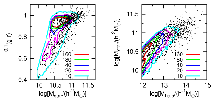
Figure 1: The colour-${\rm M_{star}}$ and ${\rm M_{star}}$-${\rm M_{halo}}$ distributions of our selected CEN sample (black circles). Contours show the distribution of all $z\leq 0.08$ CENs from the SDSS DR4 group catalogue. Contours with different colours connect bins with same number of galaxies as labelled. Each bin has a width of 0.03 in colour and 0.05 dex in ${\rm M_{star}}$ in the left panel, and a width of 0.05 dex in ${\rm M_{star}}$ and 0.06 dex in ${\rm M_{halo}}$ in the right panel.

In Figure 1, we plot the stellar mass (${\rm M}_{\rm star}$) distributions of our CEN sample as a function of galaxy colour and halo mass. For each galaxy, the NYU-VAGC provides the Petrosian ${}^{0.1}(g-r)$ colour, K+E corrected to $z=0.1$ (see Y07 for details), and we estimate ${\rm M}_{\rm star}$ using the colour-derived M/L from Bell et al. (2003). As shown in Figure 1, our representative CEN selection samples the same ${\rm M_{star}}$, ${\rm M_{halo}}$ and ${}^{0.1}(g-r)$ space as all CENs with $z\leq 0.08$ in the group catalogue (shown by the contours). We note that our selection of CENs spans a wide range of ${\rm M_{star}}$ running from $10^{9.8}$ to $10^{11.7}{\rm h^{-2}M}_{\odot}$. Owing to the exponentially decreasing number density of high-mass haloes and the ${\rm M_{star}}$-${\rm M_{halo}}$ relation of CENs (Fig.1, right panel), our selection of a constant number of groups per ${\rm M_{halo}}$ bin results in a CEN sample that is heavily-weighted towards higher stellar masses and redder colours.

2.2 Matched Satellite Galaxy Samples

In addition to studying the structural properties of CENs, we also want to investigate whether their central position in groups or clusters produces a distinctive structural difference compared to non-CEN galaxies. Following a similar method as in van den Bosch et al. (2008), we construct two control samples of satellite (SAT) galaxies, one to match CENs in stellar mass only, and the other to match in both stellar mass and colour. For each CEN in our sample, we first randomly select from all SATs with $z\leq 0.08$ a similar-mass counterpart with a ${\rm M_{star}}$ within $\pm 0.08$ dex, hereafter the SAT sample S1. We next find SATs likewise again matched to CENs in ${\rm M_{star}}$, but further restricted to match their colour within $\Delta^{0.1}(g-r)=\pm 0.03$, hereafter the SAT sample S2. Once a SAT is matched to a CEN, we remove it from the pool so that there is no duplication in each SAT sample. The matching criteria are equal to the measurement uncertainties of the stellar mass and the colour (Bell et al., 2003), and using a matching criteria with either a smaller ${\rm\Delta M_{star}}$ or $\Delta^{0.1}(g-r)$ will greatly reduce the number of matched SATs, especially towards the massive end, because we use a volume-limited sample and don’t allow duplicate matches. For CENs with ${\rm log(M_{halo}/h^{-1}M_{\odot})}<11.0$ we find a matched SAT using the above criteria more than 90 percent of the time. At higher masses (${\rm log(M_{halo}/h^{-1}M_{\odot})}>11.3$), SATs become rare and the fraction of massive CENs with a matched SAT rapidly drops to less than 10 percent. Hence, we achieve SAT samples of 769 (S1) and 746 (S2) matches.

Figure 2: The difference of ${\rm M_{star}}$ (upper panels) and colour (lower panels) between matched CENs and SATs as a function of CEN ${\rm M_{star}}$. The left column shows the differences for the SAT sample S1, which is matched with our CEN sample only in stellar mass, while the right column shows the SAT sample S2, which is matched with our CEN sample in both stellar mass and colour. The solid line in each panel shows the median of the difference for each 0.25 dex wide ${\rm M_{star}}$ bin. For comparison, circles with errorbars show the mean and 3$\sigma$ deviation of the biases in each mass bin from matching the CEN sample to 20 mock samples created from itself with random changes according to measurement uncertainties (see text for details).

In Figure 2, we plot the stellar mass and colour comparisons for our CEN-SAT matched samples as a function of CEN stellar mass. There is a slight bias in that SATs in both sample S1 and S2 are less massive than their counterpart CENs with a median difference (SAT - CEN) of -0.01 dex, and SATs in S1 are obviously redder than their counterpart CENs. The difference of colour for the SAT sample S2 (lower right panel) is also small, with an almost zero median for low mass (${\rm log(M_{star}/h^{-2}M_{\odot})}<10.5$) SAT-CEN pairs and a median of 0.005 for massive (${\rm log(M_{star}/h^{-2}M_{\odot})}>10.7$) pairs. In the lower left panel we see an obvious difference between the colour of SAT-CEN pairs in SAT sample S1, with a median difference of 0.03 for massive (${\rm log(M_{star}/h^{-2}M_{\odot}}>10.7$) pairs and 0.3 for low mass (${\rm log(M_{star}/h^{-2}M_{\odot})}<10.3$) pairs.

To evaluate whether the above biases are statistically significant or not, we match our CEN sample with mock samples created from itself with random changes on ${\rm M_{star}}$ and colour according to the measurement uncertainties. The match is done with the same criteria used for constructing the SAT sample S2 and repeated 20 times to produce a distribution of medians of $\Delta{\rm M_{star}}$ and $\Delta^{0.1}(g-r)$ per ${\rm M_{star}}$ bin between the CEN sample and mock samples. We plot the results in Figure 2 with circles and errorbars showing the mean and 3$\sigma$ deviation respectively. We can see that the biases of our real CEN-SAT matches are within 3$\sigma$ deviations of the self-matching results, except in the lower left panel, where the bias at ${\rm log(M_{star}/h^{-2}M_{\odot})}<11$ are much larger than the 3$\sigma$ deviations. This result suggests that the ${\rm M_{star}}$ and colour distributions of our SAT samples are not significantly different from the distributions of our CEN sample, except for the case of colour in our SAT sample S1, where we find that SATs are redder than their CEN counterparts as van den Bosch et al. (2008) finds. However, the colour difference between low mass CENs and SATs in sample S1 ($\Delta^{0.1}(g-r)\sim 0.3$) is larger than the average difference of $0.1$ in the same stellar mass region found by van den Bosch et al. (2008). The reason for this disagreement could be the small number statistics in our SAT sample. We conclude that the SATs from sample S2 is effectively matched in ${\rm M_{star}}$ and colour with our CEN sample, while the SATs from sample S1 are only matched in ${\rm M_{star}}$ and have a systematic redder colour than the CEN sample.

3 Measuring the Structure of Galaxies

The primary aim of this paper is to quantify the structural properties of CENs. In particular, we measure the shape and size of the 2-D luminosity profile of each galaxy using GALFIT (Peng et al., 2002). This code fits a parametric model to the surface brightness profile of a galaxy image and outputs a set of best-fitting parameters. For our analysis we adopt the Sérsic (1968) model to describe the surface brightness at radius $r$ of a galaxy, $\Sigma(r)=\Sigma_{e}e^{-b_{n}[(r/r_{50})^{1/n}-1]}$, where $r_{50}$ is the half-light radius of a galaxy, $\Sigma_{e}$ is the surface brightness at $r_{50}$, $n$ is the Sérsic index, and $b_{n}$ is coupled to $n$ such that half of the total flux of a galaxy is within $r_{50}$ (for $0.5<n<10$, $b_{n}\approx 2n-0.327$). In addition to $r_{50}$ and n, GALFIT outputs the best-fitting total magnitude ${\rm m_{tot}}$, axis ratio $b/a$, and position angle $\theta$. The Sérsic profile is routinely used for galaxy structure analysis to provide the half-light radius and the Sérsic index measures the galactic light profile shape; e.g., $n=4$ is the de Vaucouleurs’ $r^{1/4}$ profile and $n=1$ is the exponential disk profile. We choose GALFIT as our fitting tool because it can simultaneously fit Sérsic profiles to several galaxies in one image, which is advantageous for galaxies in dense environments, where galaxies have a high chance to be overlapping with one other. In what follows, we outline our image fitting pipeline, test it with simulated galaxies, discuss technical issues, and estimate the effects that background sky estimation has on parameter uncertainties.

3.1 The Galaxy Fitting Pipeline: Modified GALAPAGOS

To run GALFIT on each galaxy in our sample, we require a postage stamp image with an appropriate size to measure structure over the full extent of an object, the point spread function (PSF), the initial guess for the fitting parameters, and an estimate of the background sky level. In our pipeline, we start from the fully-processed SDSS imaging frames, which have a size of $2048\times 1042$ pixels. We employ GALAPAGOS (Barden in prep.) to process the whole image frame and to provide the needed information to GALFIT. GALAPAGOS was originally designed to facilitate fitting large galaxy data sets based on HST/ACS images. We have modified this routine to work on SDSS images. In brief, GALAPAGOS takes the following steps: (1) it detects neighbouring sources and produces image masks; (2) it cuts out postage stamps for detected sources; (3) it prepares an input file for GALFIT; and (4) it estimates local sky values for target galaxies. We outline the details of these steps below.

Source Detection and Initial Fit Parameter Guesses: We use SExtractor (Bertin & Arnouts, 1996) to detect and mask nearby companion sources in the SDSS image of each galaxy that we desire to fit, and to provide initial fit parameter guesses for the primary galaxy and any close neighbours that will be simultaneously fit. SExtractor provides useful estimates of galaxy properties (magnitude, size, axis ratio, position angle) for calculating the initial guesses for the GALFIT parameters. A set of configuration parameters defines how SExtractor detects sources. After tuning, we find that for SDSS r-band images the following configuration works best: DETECT_MINAREA=25, DETECT_THRESH=3.0 and DEBLEND_MINCONT=0.003. This configuration provides a good trade off between detecting and deblending most bright and extended sources without artificially deblending galaxies with strong substructures into multiple sources. Since our goal is to study bright galaxies in groups or clusters, we keep this configuration to allow a high success rate on bright galaxies. To distinguish whether companions are stars or galaxies, all sources with SExtractor flag STAR_CLASS$<$0.9 are classified as galaxies. However, a small fraction of sources may be misclassified using this criterion, and we will discuss the effect of this misclassification on our fitting results in §3.3.

Postage Stamp Images: GALAPAGOS produces a rectangular postage stamp centred on each galaxy of interest. The purpose of postage stamps is to reduce the CPU time for fitting one galaxy. The postage stamps are cut to a size that is large enough to ensure that the outer light profile will be fit. GALAPAGOS uses parameters in the SExtractor catalogue to determine the X and Y dimension in pixels of the postage stamps for each object:

$$X=2.5\times a\times r_{Kron}\times(|sin(\theta)|+(1-e)|cos(\theta)|),$$ (1)

$$Y=2.5\times a\times r_{Kron}\times(|cos(\theta)|+(1-e)|sin(\theta)|),$$ (2)

where $a\times r_{Kron}$ is the Kron radius along the major axis in units of pixels, $\theta$ is the position angle, and $e$ is the ellipticity.

GALFIT Inputs: For running GALFIT, GALAPAGOS produces an input file of initial parameter guesses for the fitting parameters based on the SExtractor output as follows: ${\rm m_{tot,i}=MAG\_BEST}$ for the apparent $r$-band magnitude, ${\rm r_{50,i}}=0.162r_{flux}^{1.87}$, where $r_{flux}$ is FLUX_RADIUS; ${b/a}_{i}=1-e$, where $e$ is ELLIPTICITY; and $\theta_{i}={\rm THETA\_IMAGE}$. We start with an initial Sérsic index of $n=1.5$. We note that for this analysis, we do not use the higher fitting modes, such as diskyness and boxiness, offered with the GALFIT software. Nearby companions within 1.5 times the SExtractor Kron aperture of the target galaxy are fit simultaneously with a Sérsic model using initial parameters also determined as described above. Companions further away are masked out using the masks provided by SExtractor. In addition to the input file, GALFIT requires a PSF image to convolve with the model image. The PSF at the centre of the target galaxy is extracted from the SDSS photo pipeline by employing a SDSS published tool readAtlasImages.

Background Sky Estimation: The background sky level is a critically important ingredient in galaxy image fitting. For example, an overestimation of the sky can result in flux, size, and Sérsic index underestimation. GALAPAGOS includes a sophisticated way to measure the local sky around a galaxy, which is demonstrated to be successful for ACS images (Häussler et al., 2007). However, GALAPAGOS uses a hierarchical iteration for fitting galaxies, from bright to faint, over the whole frame to isolate sky pixels. Rather than using this CPU-intensive approach, we rely on the SDSS, which provides useful and well-tested sky estimates. The SDSS global sky is considered to be a good measure of the background sky level for studying the structure of SDSS galaxies (von der Linden et al., 2007). We treat the background sky as a fixed flux pedestal during the fitting to reduce degeneracies between the sky and the outer isophotes of high-$n$ models.

3.2 Testing the Pipeline with Simulations

We test our SDSS image fitting pipeline by running it on 850 simulated galaxies. The goals of this test are two fold: (1) to estimate random and bias of the structural parameters returned by our fitting pipeline; and (2) to confirm that using the SDSS global sky does not produce bias. We compare the actual properties that define each simulated galaxy (input) to the corresponding fit result (output) following Figure 9 in Blanton et al. (2005).

For our tests, we use the SDSS-based simulations of Blanton et al. (2005). Briefly, each simulated galaxy is an axisymmetric Sérsic model. The simulation sample has a range of input parameters matching the NYU-VAGC Large-Scale Structure (LSS) sample from SDSS DR4. Each simulated galaxy is converted to raw data units, scaled to the SDSS pixel size, and convolved with the PSF at its position. After adding Poisson noise, the resulting image is placed into an actual SDSS image at a random location. Generally, about 60 simulated galaxies were added to each $2048\times 1024$ pixel image.

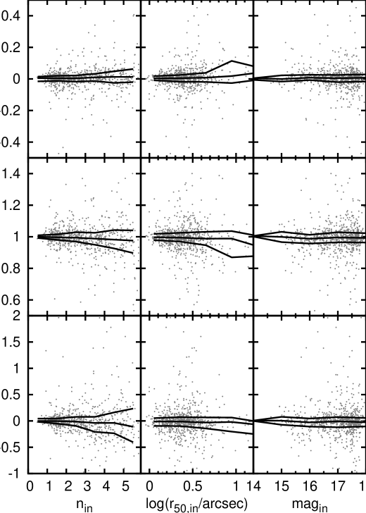
Figure 3: A comparison between input and output parameters when using GALFIT to fit Sérsic models to 850 simulated Sérsic galaxies. We plot the difference (output-input) as a function of input for three important Sérsic parameters: the index $n$, the half-light radius $r_{50}$, and the total magnitude. In each panel, grey points represent individual simulated galaxies. The solid lines show the 3rd quartile, median and 1st quartile (from top to bottom).

The results of applying our pipeline to the SDSS simulations are shown in Figure 3. We plot the output-input offset as a function of input for three important parameters: the total magnitude ${\rm m_{tot}}$, the half-light radius $r_{50}$, and the Sérsic index $n$. The results demonstrate that our pipeline successfully recovers these structural parameters of simulated Sérsic galaxies with almost no offset and only a small scatter. For half of the simulation sample the pipeline returns structural measurements within 10 percent of the true value. As expected, there is a larger parameter offset scatter for simulated galaxies with $n_{in}>4$ than for those with $n_{in}<4$ (see Häussler et al. (2007)). We see a slightly increased scatter with magnitude owing to the lower S/N of fainter galaxies. We note that the good agreement between input and output parameters also demonstrates that the SDSS global sky is a good choice for galaxy image fitting. We address the effects of sky uncertainties on our structural properties measurements in more detail in §3.4. To the degree that Sérsic profiles provide a reasonable fit to the true light distribution of galaxies, the good performance of our pipeline on simulated galaxies is promising for the analysis of real galaxies.

3.3 Sérsic Fitting of the CEN Sample

We apply our pipeline to fit each galaxy in the CEN sample with a Sérsic model. To evaluate the fit quality we visually checked a random subsample of 200 CENs and find that about 15 percent of our fits suffer from a variety of technical issues. These issues include stars misclassified as galaxies and unreliable fits to companion sources. Here we discuss what portion of our fitting results are affected by these issues and how we can correct for them.

The accuracy of star/galaxy classification affects the fitting quality. Although CEN galaxies can always be correctly classified, a small portion of their companions may suffer from misclassification. Some galaxies are misclassified as stars and some stars are misclassified as galaxies, but only the latter has a severe impact on our fitting. Fitting a Sérsic model to a stellar profile typically results in a very large $n$ with an overestimated extent and an overestimated flux. As a result, this false extension takes light away from the whole image and hence causes an underestimate of ${\rm m_{tot}}$, $r_{50}$ and $n$ for the target galaxy. Conversely, companion galaxies misidentified as stars and fit by a PSF are spatially compact and faint, thus their improper treatment has little impact on the measured structure or flux of the target galaxy. We estimate that less than 5 percent of our CEN sample (in a random sense) suffer from the issue of companion stars being misclassified as galaxies.

A drawback to fitting several sources simultaneously is that an unrealistic model fit for a companion will spoil the fitting quality of the target galaxy. We develop an empirical set of criteria for identifying bad companions such that any companion being fitted with $\sigma_{{\rm a_{50}}}/{\rm a_{50}}>0.3$ and $n>8.0$ is identified as a bad companion, where ${\rm a_{50}}$ is the semi-major axis ${\rm a_{50}}=r_{50}/\sqrt{b/a}$, $b/a$ is the axis ratio, and $\sigma_{\rm a_{50}}$ is the internal GALFIT error of ${\rm a_{50}}$. Such bad companions are usually small and/or low surface brightness galaxies and tend to be fit with an overestimated size, Sérsic index and magnitude, resulting in a severe underestimate of the same quantities for the target galaxies. We examine SExtractor magnitude differences between bad companions ($m_{BC}$) and target galaxies ($m_{T}$) and find that bad companions, as defined here, are mostly fainter than their corresponding targets. Actually, the majority of bad companions have $\Delta m=m_{BC}-m_{T}>2.5$ and the distribution of $\Delta m$ is peaked at $\Delta m\sim 3.5$. Thus we simply mask out all $\Delta m>2.5$ bad companions and refit the image. We iterate this procedure until all the targets have no more bad companions. About 8 percent of our CEN sample start with bad companions and we correct all of them as described above. Some of the target CENs have $\Delta m<2.5$ bad companions within a few arcseconds and any masking might adversely affect the fit. Hence instead we opt to exclude those target galaxies from our CEN sample. The fraction of CENs having such bad companions depends on halo mass: from 7 percent at high-masses to 3 percent at low-masses. In total, 32 CENs are excluded from our sample owing to problems with bad companions.

3.4 Sky Uncertainty and Parameter Covariance

Although the SDSS global sky works as a good choice of sky background for fitting isolated galaxies, as the simulations show, the real sky is difficult to measure especially for CENs in dense environments. In this subsection, we estimate the uncertainty in the SDSS global sky values and evaluate how this uncertainty translates into fit parameter errors.

We use the difference between the SDSS global sky and mean sky to characterise the uncertainty in the sky measurement. SDSS measures the global sky as the median data counts (ADUs) from every pixel of the source-subtracted frame after sigma-clipping. Besides the global sky, SDSS also provides a mean sky for each frame and a local sky for each detected object in the frame. SDSS measures the background in sub-frame boxes of of $256\times 256$  pixels centred every 128 pixels. The local sky of each object in a SDSS frame is an interpolation of the sub-frame background values at the position of the object centre. The mean of all sub-frames is the mean sky for a frame.

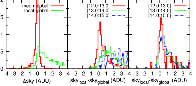
Figure 4: Distributions of differences between various sky measurements. Left: The red line shows the difference between the SDSS mean and global sky values for our CEN sample and the green line shows the difference between the SDSS local and global measurements. Middle: The local-global difference for CENs divided into halo mass bins. Right: Same as the middle panel, but for SATs.

In the left panel of Figure 4, we plot the difference between the SDSS global sky and mean sky for our CEN sample. The mean sky is somewhat larger than the global sky on average because individual sub-frames may suffer contamination from large and bright sources. We also plot the difference between the SDSS global and local sky measurements for our sample in the left panel. These differences are much larger than that between the global and mean sky because the local sky is heavily contaminated by large and bright sources. Furthermore, in the middle panel of Figure 4, we show that the overestimates of the local sky are halo-mass dependent for CENs. The local sky at the centre of massive haloes tends to be higher than that in less massive haloes. Since the real sky background should be independent of the properties of haloes, this dependence implies that local sky measures for CENs suffer from increased contamination from the higher density of galaxies in larger haloes. In contrast, SATs display little dependence on halo mass, even though their local sky is also overestimated, as shown in the right panel of Figure 4. We attribute this lack of halo dependence to the fact that SATs are found over a range of halo-centric positions and hence at various galaxy densities. It is also possible that intra cluster light (ICL) at the centre of massive haloes can contribute to the difference between CEN and SAT sky estimates as we show in Figure 4. Given the large overestimates and the halo dependence of the SDSS local sky, we will not use it as a measurement of the sky background. Moreover, we conclude that the SDSS mean sky not only provides a robust alternative measurement of the sky background but it also tells us in which direction the sky measurement might be biased.

To study the effect of sky uncertainties on the Sérsic fitting of actual galaxies, we first select a representative subset of 45 CENs from our sample that span a $3\times 3$ matrix in ${\rm M_{halo}}$-$n$ space as follows:

• for ${\rm log(M_{halo}/h^{-1}M_{\odot})}$=[12.0:12.5], n=[1.8:2.2], [3.3:3.7], [4.8:5.2]

• for ${\rm log(M_{halo}/h^{-1}M_{\odot})}$=[13.0:13.5], n=[2.8:3.2], [4.3:4.7], [6.3:6.7]

• for ${\rm log(M_{halo}/h^{-1}M_{\odot})}$=[14.0:14.5], n=[3.8:4.2], [4.8:5.2], [6.3:6.7]

Next, we randomly select five galaxies from each bin of the above matrix. For each galaxy, we Monte-Carlo sample 50 values from the distribution of the mean-global difference shown by the red line in the left panel of Figure 4. These values are added to the global sky and the galaxy is refit using these new background levels. This procedure provides a distribution of fitting parameters caused by the uncertainty in measuring the sky. For this subset of 45 CENs, we plot distributions around the mean value of three important fit parameters ($m_{\rm tot}$, $n$ and ${\rm a_{50}}$) in Figure 5.

The distributions in Figure 5 clearly demonstrate a covariance between best-fitting parameter values and the choice of sky. The boxes represent our original results using the SDSS global sky. The series of (50) crosses, which form a short and nearly straight line through each box, represent the fitting results using the Monte Carlo sampling of the sky background as described above. The correlations between ${\rm m_{tot}}$ and ${\rm a_{50}}$ (bottom) and ${\rm m_{tot}}$ and $n$ (top) show the strong degeneracy of these parameters in the Sérsic model. If we increase the sky background, the best-fitting flux decreases to keep the total (galaxy + sky) flux constant, while the best-fitting $n$ and ${\rm a_{50}}$ decrease. Conversely, decreasing the sky background level results in larger best-fitting values for ${\rm m_{tot}}$, $n$, and ${\rm a_{50}}$. We find that the covariance is more severe for galaxies with higher $n$. This effect shows that the sky estimate is very crucial for producing accurate Sérsic profile fits. This is especially true for galaxies with $n>4$ because the flat, extended wings of the profile are sensitive to sky uncertainties. The strength and direction of these covariances must be accounted for when analysing the size-luminosity relation, as we will discuss in §4.2

Figure 5: The covariances among best-fitting total magnitude, Sérsic index and ${\rm a_{50}}$ as a result of sky uncertainty for 45 representative CENs. Boxes represent the GALFIT result using the SDSS global sky. For each galaxy, the series of (50) crosses represent fits using sky background levels taken from Monte Carlo samplings of the sky as described in the text.

4 The Structure of CENs

In this section we explore the r-band structural properties of our CEN sample. CENs are the most massive members of the SDSS groups and clusters, and are presumed to be located at the dynamical centre of the host halo. We focus on the structural shape (characterised by the Sérsic index $n$) and the size (characterised by the half-light radius $r_{50}$) of the Sérsic profile of CENs. We study the relationships between these parameters and galaxy stellar masses and host halo masses to investigate which factor is more related to the structure of CENs. We also compare the structural parameters of CENs and SATs using our two matched SAT samples (see §2 for details) and study whether the central halo location impacts the shape or size of a galaxy.

To evaluate the accuracy of our measurements of galaxy structural parameters and total flux using our GALFIT pipeline, we compare our fit results with the one-dimensional (1D) Sérsic fitting parameters based on the NYU-VAGC analysis (Blanton et al., 2005, hereafter ’NYU-VAGC’). The NYU-VAGC Sérsic parameters have been widely used in the study of galaxy morphology and size (e.g. Shen et al., 2003; Blanton et al., 2005; Maller et al., 2008). We find that for high Sérsic index (our GALFIT $n>3.0$) galaxies, NYU-VAGC underestimates the Sérsic index by about 1.3 and underestimates the total magnitude by about 0.4 mag compared to our results. There are two reasons for these underestimates: (1) NYU-VAGC’s 1D profile fitting systematically underestimates the Sérsic index and total magnitude for high $n$ galaxies, as shown by Figure 9 of Blanton et al. (2005); (2) NYU-VAGC uses the SDSS local sky, which overestimates the background sky level and hence results in underestimates of $n$ and the total magnitude. Furthermore, for low Sérsic index (our GALFIT $n<3.0$) galaxies, NYU-VAGC overestimates the Sérsic index but still underestimates the total magnitude by about 0.2 mag. Besides using the local sky, NYU-VAGC’s azimuthally-averaged 1D fitting procedure systematically overestimates the Sérsic index for highly inclined galaxies, which are mostly disks. We also compare both our GALFIT results and the NYU-VAGC results with the Petrosian quantities from the SDSS photometric pipeline. By following the formalism of Graham et al. (2005), we find that under our working assumptions (a Sérsic model and a global sky), our GALFIT fitting pipeline more accurately measures the structural properties of SDSS galaxies then NYU-VAGC’s. The details of this comparison are in Appendix A.

4.1 The Sérsic Index of CENs

With reliable and accurate measurements of galaxy structural properties from our fitting pipeline in hand, we turn to the study of how the Sérsic index of CENs is related to their stellar mass and their environment. The Sérsic index is widely used to characterise the profile and concentration of galaxies in both observational (e.g., Graham et al., 1996; Blanton et al., 2005; MacArthur et al., 2003; de Jong et al., 2004; Allen et al., 2006) and numerical (e.g., Naab & Trujillo, 2006; Aceves et al., 2006) studies. Some argue that the morphology-density relation implies that the structure of galaxies is affected by the environment. Others argue that the structure of galaxies depends strongly on stellar mass but only weakly on the environment (e.g., Hogg et al., 2004; Kauffmann et al., 2004; van der Wel, 2008). In this section, we explore the dependence of the Sérsic -index distribution of CEN galaxies on both ${\rm M_{star}}$ and ${\rm M_{halo}}$.

4.1.1 Dependence on Stellar Mass

In the upper left panel of Figure 6, we plot the Sérsic index of CENs as a function of their stellar mass. The ${\rm M_{star}}$ values for our CEN sample are calculated following the formula from Bell et al. (2003):

$${\rm log}[{\rm M}_{\rm star}/{\rm M}_{\sun}]=-0.306+1.097^{0.0}(g-r)-0.15-0.4(^{0.0}M_{r}-4.67),$$ (3)

where the constant 0.15 corrects to a Kroupa (2001) IMF, and ${}^{0.0}(g-r)$ is the Petrosian colour from the NYU-VAGC shifted to the $z=0$ rest-frame using the Blanton et al. (2003) $K$-corrections and correcting for Milky Way extinction using the Schlegel et al. (1998) dust maps. The absolute $r$-band magnitude ${}^{0.0}M_{r}$ is extinction and K-corrected in the same manner, but we use the total flux from our fitting for this quantity rather than the Petrosian magnitude in the SDSS pipeline. We show in Appendix A that our fitting procedure better recovers the total magnitude of galaxies than the Petrosian photometry. The red symbols with errorbars in Figure 6 show the median and the 1st and 3rd quartile of the $n$ distribution in ${\rm M_{star}}$ bins with a 0.25 dex width. From the plot we see that the median Sérsic index is a strong function of stellar mass: low-mass CENs have low $n$ (disk-like) and high-mass CENs have high $n$ (spheroid-like). Yet, there is large scatter in the relation between $n$ and ${\rm M_{star}}$ , especially for CENs with $3\times 10^{10}<{\rm M_{star}/h^{-2}M_{\odot}}<10^{11}$, where the Sérsic index ranges from $1<n<6$ or larger. Higher-mass CENs tend to have $n>3$.

We also show how the uncertainty and covariance of the GALFIT $n$ values affect the $n$-${\rm M_{star}}$ relation in the upper left panel of Figure 6 (green symbols). The red symbols in the plot only take into account of the scatter from our fits. However, as we showed in §3.4, there is a strong covariance between the fit parameters $n$ and $m_{\rm tot}$ and the sky uncertainty, and we use $m_{\rm tot}$ to estimate stellar mass. To evaluate how this covariance may change the above $n$-${\rm M_{star}}$ relation, we re-calculate the relation using the results from the representative subset of 45 CENs in §3.4. For each CEN in our sample we randomly select one CEN from the nearest five in $n$ space among the representative subset, and we assume that each CEN has the same $n$ and $m_{\rm tot}$ covariance as its matched companion. In this way, we construct a probability distribution of $n$ and ${\rm M_{star}}$ (from $m_{\rm tot}$) for all 911 CENs. The median, 1st and 3rd quartiles of this distribution are shown by the green symbols and errorbars in the upper left panel of Figure 6. The new relation shows little difference compared with the original because the parameter uncertainties owing to sky are smaller than the intrinsic scatter in our sample (red symbols). For example, the average relative scatter between the 1st and 3rd quartiles of $n$ owing to the background sky level uncertainty is only $\Delta n/n\sim 0.2$, while the measured scatter is $\Delta n/n\sim 0.75$ and hence dominates.

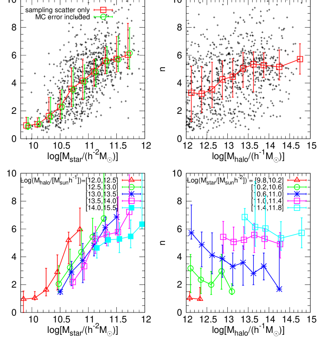
Figure 6: Upper left: the relation between Sérsic index and stellar mass for our CEN sample. Black crosses represent the best-fitting $n$ for individual CEN galaxies. The red line connects the median (open squares) of the $n$ distribution in each ${\rm M_{star}}$ bin. The green line and open circles show the median once the $n$ and $m_{\rm tot}$ fitting uncertainties owing to sky are folded into the distribution (see text for details). The errorbars show the first and third quartiles. Upper right: the relation between the best-fitting Sérsic index and halo mass for our CEN sample. Black crosses and red lines with errorbars are done as in the left panel. Lower left: the $n$-${\rm M_{star}}$ relation split into different bins of fixed halo mass as indicated by key. Lower right: the $n$-${\rm M_{halo}}$ relation split into different bins of fixed stellar mass as indicated by the key. In both lower panels, the symbols and errorbars provide the median, 1st, and 3rd quartiles. In the lower panels, only the best-fitting results are used.

4.1.2 The Dependence on Host Halo Mass

In the upper right panel of Figure 6, we show the dependence of the Sérsic index of CENs on their host halo mass. Recall that ${\rm M_{halo}}$ is calculated by matching the rank of the total stellar mass of groups and clusters with that of dark matter haloes from numerical simulations (see Y07 for details). We find that $n$ depends only weakly on ${\rm M_{halo}}$ and that the scatter of the $n$-${\rm M_{halo}}$ relation is large. For CENs in haloes with ${\rm log[M_{halo}/h^{-1}(M_{\odot})]<12.5}$, we find a median value of $n=3$ and a relative scatter of $\Delta n/n\sim 1.3$. For massive haloes with ${\rm log[M_{halo}/h^{-1}(M_{\odot})]>14.0}$ the median is $n=5$ and the relative scatter is $\Delta n/n\sim 0.6$.

The $n$-${\rm M_{halo}}$ relation, although weak, suggests that the halo mass may also affect the structure of CENs. However, from the right panel of Figure 1 we know that the stellar mass of CENs also depends on the halo mass in the sense that CENs in massive haloes tend to have larger stellar masses than CENs in smaller haloes. Given this dependence and the strength of the $n$-${\rm M_{star}}$ relation, it is tempting to rule out any dependence of $n$ on halo mass. To address this, we attempt to remove any ${\rm M_{star}}$ -${\rm M_{halo}}$ dependence from both the $n$-${\rm M_{star}}$ and $n$-${\rm M_{halo}}$ relations.

First, in the lower left panel of Figure 6, we plot the $n$-${\rm M_{star}}$ relations for CENs in five halo mass bins, each 0.5 dex in width. All the bins with less than six CENs are excluded to get better statistics. The roughly ${\rm M_{halo}}$ -independent relations all have a slope and amplitude that is similar to the single $n$-${\rm M_{star}}$ relation for the full sample (red symbols in the upper left panel). There is some evidence that the relations for different ${\rm M_{halo}}$ bins are somewhat offset along the ${\rm M_{star}}$ direction in the sense that CENs in less massive haloes tend to have larger $n$ than their counterparts in more massive haloes. But since the scatter in the relations are large, we cannot draw any firm conclusions.

Similarly, we study the $n$-${\rm M_{halo}}$ relations of CENs in five different ${\rm M_{star}}$ bins, each with a width of 0.4 dex, as shown in the lower right panel of Figure 6. We find that the $n$-${\rm M_{halo}}$ relations for each bin of fixed galaxy mass is different from the single $n$-${\rm M_{halo}}$ relation for the full sample. For the most part, the relations are all flat, i.e. each CEN of a given ${\rm M_{star}}$ has a constant $n$, within the scatter, independent of its host halo mass. We note that several of the fixed stellar mass relations have a small negative slope when considering only the median values. This slight trend is a manifestation of the small offsets among the $n$-${\rm M_{star}}$ relations in different ${\rm M_{halo}}$ bins in the lower left panel. A much larger sample is required to validate whether the profile shape of CENs, as measured with Sérsic fitting, has a small second-order dependence on halo mass.

4.1.3 Discussion

We study the distribution of $n$ for our CEN sample and its dependence on ${\rm M_{star}}$ and ${\rm M_{halo}}$ and find that the Sérsic profile shape of CENs is strongly correlated with ${\rm M_{star}}$ but only weakly (or not at all) correlated with ${\rm M_{halo}}$. Low-mass CENs tend to have shallower, disk-like profiles, while massive CENs have steeper, more spheroid-like shapes. This $n$-${\rm M_{star}}$ relation holds for CENs from different ${\rm M_{halo}}$ bins with almost the same slope and amplitude. On the other hand, CENs have $n$ values that depend very weakly, if at all, on global environment as defined by ${\rm M_{halo}}$, which is consistent with other observations (Kauffmann et al., 2004; van der Wel, 2008). This correlation disappears (or even becomes an anti-correlation) if we divide our CEN sample into different ${\rm M_{star}}$ bins. This suggests that ${\rm M_{halo}}$ has almost no effect on the shape or concentration of CENs. The key factor that determines $n$ of a CEN is its stellar mass. Given the relationship between the masses of CENs and their host halo masses, the phenomenon of CENs in massive haloes having a more concentrated structure (as implied by morphology-density relation) can be explained simply by (1) an intrinsic $n$-${\rm M_{star}}$ correlation, and (2) massive CENs living preferentially in massive haloes (i.e., mass segregation).

We find low-$n$ (disk-like) CENs in haloes spanning a large range in halo mass (from $10^{12}$ to ${\rm 10^{14}h^{-1}M_{\odot}}$), which rules out a distinct (special) ${\rm M_{halo}}$ for producing spheroids. Likewise, finding high-$n$ (early-type) CENs over the same range of environments suggests that major mergers, or some other processes that transforms disk galaxies into spheroid-like galaxies, occur at the centres of haloes with a wide range of masses. Finally, it is unclear whether the halo plays a small, secondary role in determining the overall profile shape of its CEN as hinted at in the bottom panels of Figure 6. The ${\rm M_{star}}$ -${\rm M_{halo}}$ relation in Figure 1 shows that CENs of a fixed stellar mass reside in haloes with a range of masses. We speculate that the tendency for CENs of a fixed stellar mass to be more concentrated in smaller haloes and less so in larger haloes may tell us something about the recent accretion history of the host and its impact on the stellar mass growth of the CEN. Halos grow through the accretion of, and the merging with, other haloes. Briefly, consider two haloes (A and B) that were equal in mass and contained similar central disk galaxies in the recent past. Since that time both haloes have doubled in mass, halo A by a single major merger with a comparable halo, and B by accreting many minor subhaloes. Owing to dynamical friction timescales, the disk CEN in halo A will both (i) grow in mass faster than halo B’s CEN and (ii) be transformed into a spheroid because it is doomed to experience a major merger with the CEN of the merging halo. Conversely, the mass of the CEN in halo B will take much longer to grow by the occasional minor merger with small infalling companions, and this process is much less likely to destroy its disk morphology. Therefore, when comparing haloes of the same mass, galaxies that grew through major mergers will be more massive and more concentrated. Likewise, when comparing CENs of the same stellar mass, those which grew through major mergers (i.e., more concentrated) will reside in lower mass haloes on average more than their disk-dominated counterparts as we see in the lower left panel of Figure 6. Numerical modelling and a more-detailed analysis on a much larger data set could test these predictions.

4.2 The Size of CENs

In addition to the Sérsic index, the half-light size is an important characteristic of galaxy structure. It is well-established that galaxies follow well-defined size-luminosity ($r_{50}$-$L$) and size-stellar mass ($r_{50}$-${\rm M_{r}}$) relations (e.g. Shen et al., 2003; Bernardi et al., 2007; Dutton et al., 2007), which are commonly used to constrain galaxy formation and evolution theories. In this subsection, we study the size-luminosity relation and the size-stellar mass relations of our CEN sample and compare our results with those obtained by others. Our CEN sample contains both early and late-type galaxies. Thus, we visually inspect each galaxy and divide the sample into two types based on whether spiral disk structure is present (late-type) or not (early-type). In Figure 7 we plot the distribution of our best-fitting Sérsic index for our visual inspected early- (solid line) and late-type (dotted line) CENs. Unlike employing a sharp cut at $n=2.5$ as in many studies, the majority of our early-type CENs have $n>3.5$, while late-type CENs have $n<3.5$. In what follows, we will discuss the early and late-type size-luminosity and size-stellar mass relations separately.

Figure 7: The distribution of Sérsic index for our visual inspected early- (solid line) and late-type (dotted line) CENs. The Sérsic index comes from our best fits.

Figure 8: The size-luminosity (left) and size-stellar mass (right) relations for early-type (upper) and late-type (lower) galaxies in our CEN sample. The thick solid line in each panel is the best fit linear relation for each morphological type over the whole luminosity/stellar mass range. The dashed line in each panel shows the linear relation by fitting the faint end (${\rm M_{r}-5log(h)\geq-22}$). For comparison, the thin dotted line in each panel is the relation from S03 (see the text for details). The arrow in the upper right panel shows the direction and amplitude of the average covariance between ${\rm M_{r}}$ and $r_{50}$ for bright (${\rm M_{r}-5log(h)<-22}$) CENs owing to background sky uncertainties (see §3.4 for details).

In Figure 8, we show the size-luminosity relation of early- (the upper left panel) and late-type (the lower left panel) CEN galaxies. Here we use the half-light radius $r_{50}$ (in units of ${\rm h}^{-1}$ kpc) to represent the size of a galaxy. We have $r_{50}=\frac{\pi}{180}\times\frac{{\rm a_{50}}}{3600}\times\sqrt{b/a}\times dA(z)$, where ${\rm a_{50}}$ and $b/a$ is the semi-major axis and the axis ratio of our best-fitting model of the galaxy, $dA(z)$ is the angular diameter distance at redshift $z$ of the galaxy. We calculate the absolute magnitude using the total magnitude from our Sérsic fit, K+E corrected to $z=0.1$. Following Shen et al. (2003, hereafter S03), who also measured the $r_{50}$-$L$ or $r_{50}$-${\rm M_{r}}$ relation for SDSS galaxies, we use linear regression to fit the $r_{50}$-$L$ relation, i.e. ${\rm log[{\it r}_{50}/(h^{-1}kpc)]=-0.4\alpha M_{r}+\beta}$. We find slopes of $\alpha=1.02\pm 0.03$ for early-type CENs and $\alpha=0.88\pm 0.04$ for late-type CENs. The linear fits are shown by thick solid lines in each panel.

At the bright end, ${\rm M_{r}-5\log{h}}<-22$, the relation steepens. The origin of this steepening is unclear. It could be caused by the covariance between the semi-major axis ${\rm a_{50}}$ and the total magnitude ${\rm m_{tot}}$, as shown in the upper panel of Figure 5. Our tests in §3.4 show that there is a very strong covariance between ${\rm a_{50}}$ and ${\rm m_{tot}}$, owing to uncertainties in the measurement of background sky level, and that this covariance becomes stronger for bright and large galaxies. The covariance between ${\rm a_{50}}$ and ${\rm m_{tot}}$ will produce a covariance between $r_{50}$ and ${\rm M_{r}}$ in Figure 8 since ${\rm M_{r}}$ is calculated from ${\rm m_{tot}}$. The direction of the average covariance at the bright magnitude end, as shown by the arrow in the upper left panel of Figure 8, is almost parallel to the slope of the relation at the bright end. Moreover, the amplitude of the covariance increases for brighter and larger galaxies as seen in Figure 5. Hence the covariance between size and total magnitude in the profile fitting could contribute to the slope steepening at the bright end.

To account for any bias at the bright end, we refit excluding sources with ${\rm M_{r}-5\log{h}<-22}$ and find slopes of $\alpha=0.82\pm 0.06$ (early-type) and $\alpha=0.57\pm 0.04$ (late-type). For reference, a fit to the $r_{50}$-$L$ relation of early-type CENs brighter than -22 has a slope of $\alpha=1.32\pm 0.08$. We don’t fit the bright end of late-type CENs, because there are only several galaxies. Using the fit over the faint end (${\rm M_{r}-5\log{h}\geq-22}$), we find an early-type $r_{50}$-$L$ relation with a much steeper slope than the $\alpha=0.65$ of S03 (the thin dotted line in the upper left panel of Figure 8). Our fit to the $r_{50}$-$L$ relation for late-type CENs fainter than -22 is also qualitatively steeper than that of S03 (comparing the dashed and dotted line in the lower left panel), who fit the $r_{50}$-$L$ relation with a four-parameter model. We note that the definition of early/late types in S03 is different from ours. They classified galaxies with a Sérsic index $n>2.5$ as early-type and the others as late-type. The different definitions of early/late-type between S03 and us could contribute to the measured slope differences. We also try the same early/late-type classification as S03 by using Sérsic index from our best fits and refit the $r_{50}$-$L$ relation for the faint end CENs. We find $\alpha=0.78\pm 0.05$ for the slope of early-type CENs, which becomes flatter due to containing more low Sérsic index galaxies than our visually inspected early-type sample but is still steeper than the slope of S03. There are two other possible reasons for the large discrepancies in slope between the $r_{50}$-$L$ relation of S03 and our result: (1) S03 use the results of an early version of the NYU-VAGC fitting, which underestimates both the total flux and the size of galaxies, as shown in Appendix A; (2) S03 covers a wide range of luminosity and hence contains many faint (fainter than the faintest one in our sample) galaxies. The slope of the $r_{50}$-$L$ relation could have a smooth transition from a flat one at the faint galaxy end to a steep one at the luminous galaxy end, as suggested by Desroches et al. (2007). Including many faint galaxies in the S03’s sample can flatten the average slope of the whole sample, making their slope smaller than ours.

We also compare our results with other studies of the $r_{50}$-$L$ relation of BCGs, a subset of massive early-type galaxies at the centres of large clusters. Bernardi et al. (2007) fit a de Vaucouleurs model to SDSS images of BCGs from the C4 cluster catalogue (Miller et al., 2005) and study the $r_{50}$-$L$ relation by using the half-light radius of their best-fitting models. They find a slope of $\alpha=0.89$ for early-type BCGs over the luminosity range of ${\rm M_{r}-5log(h)}=[-20.3:-23.3]$. This slope is a bit shallower than our slope ($\sim 1.0$) for early-type CENs over the same luminosity range. The difference could be attributed to the fact that they fit BCGs with a de Vaucouleurs profile rather than a Sérsic profile, which yields a smaller size and hence results in a flatter $r_{50}$-$L$ relation, as shown in their paper. von der Linden et al. (2007) performed isophotal photometry on the SDSS BCGs from the C4 cluster catalogue (Miller et al., 2005) and found $\alpha=0.65\pm 0.02$ for BCGs over the luminosity range ${\rm M_{r}-5log(h)}=[-20.3:-23.3]$. However, the isophotal photometry technique could miss the extended outer parts of galaxy light profiles and hence result in underestimates of both $r_{50}$ and $L$. Lauer et al. (2007) combined surface photometry presented in several HST imaging programs for 219 early type galaxies and fit them using a de Vaucouleurs profile. They found $\alpha=1.18\pm 0.06$ for galaxies with ${\rm M_{V}}<-21$ and that the $r_{50}$-$L$ relation changed from a flat slope to a steep slope at around $M_{V}=-22$. This slope is close to our slope for CENs brighter than ${\rm M_{r}-5log(h)}=-22$. Also, their slope behaves qualitatively like ours, with a steep slope at the bright end and a more shallow slope at the faint end. Gonzalez et al. (2005) fit Sérsic profiles to the I-band images of 24 luminous BCGs residing in large clusters and found $\alpha=1.8\pm 0.2$, but these fits included significant ICL. During our tests in §3.4, we showed the sensitivity to the background sky estimate and the covariance of the size and magnitude from profile fitting. This could become more acute for high luminosity CENs, where distinguishing the ICL from the extended outer light bound to a galaxy becomes increasingly difficult.

Overall, although it is well known that size strongly correlates with luminosity, the slope of this relation is hard to determine precisely. As we summarised in Table 1, authors with different samples, measurement techniques, definitions of size and/or even the criteria to split their samples into early and late types obtain different slopes. What’s more, a small uncertainty in background sky translates into a strong covariance between size and luminosity and hence can change the slope, especially for bright and large galaxies. Based on our analysis of the robustness and uncertainty of our fitting, and combined with previous work, we propose slopes for the $r_{50}$-$L$ relation of $\alpha\sim 0.9$ and $\alpha\sim 0.6$ for early-type and late-type CENs, respectively.

Table 1: Slope of the $r_{50}$-$L$ relation for early-type galaxies from various authors

Work	Sample	$\alpha$	$\Delta\alpha$	Luminosity range	Model
This work	Y07 CENs	1.02	$\pm 0.03$	${\rm M_{r}-5log(h)}=[-19:-24]$	Sérsic
This work	Y07 CENs	0.82	$\pm 0.06$	${\rm M_{r}-5log(h)}>-22$	Sérsic
This work	Y07 CENs	1.32	$\pm 0.08$	${\rm M_{r}-5log(h)}<-22$	Sérsic
Shen et al. (2003)	SDSS galaxies	0.65	–	${\rm M_{r}-5log(h)}=[-15.3:-23.3]$	Sérsic
von der Linden et al. (2008)	C4 BCGs	0.65	$\pm 0.02$	${\rm M_{r}-5log(h)}=[-20.3:-23.3]$	isophotal photometry
Bernardi et al. (2007)	C4 BCGs	0.89	–	${\rm M_{r}-5log(h)}=[-20.3:-23.8]$	de Vaucouleurs
Lauer et al. (2006)	219 galaxies	1.18	$\pm 0.06$	${\rm M_{V}}<-21$	de Vaucouleurs
Gonzalez et al. (2006)	24 BCGs	1.8	$\pm 0.2$	${\rm M_{I}}<-24$	Sérsic

Closely related to the size-luminosity relation of CEN galaxies is their size-stellar mass $r_{50}$-${\rm M_{star}}$ relation. For comparison, we plot the $r_{50}$-${\rm M_{star}}$ relations for our early-type (upper right) and late-type (lower left) CENs in Figure 8. We find slopes of $\alpha=0.90\pm 0.02$ (early-type) and $\alpha=0.47\pm 0.03$ (late-type) by using the relation ${{\rm log[}r_{50}{\rm/(h^{-1}kpc)]=\alpha log[M_{star}/(h^{-2}M_{\odot})]+\beta}}$ to fit the whole luminosity/stellar mass range of our CEN sample. Similar to the $r_{50}$-$L$ relations, our $r_{50}$-${\rm M_{star}}$ relations are steepened by the covariance between size and total magnitude in the profile fitting. We also refit the relations with bright (${\rm M_{r}-5log(h)<-22}$) CENs excluded and find slopes of $\alpha=0.68\pm 0.03$ (early-type) and $\alpha=0.35\pm 0.03$ (late-type). Our slopes of faint end (${\rm M_{r}-5log(h)\geq-22}$) CENs are steeper than those in S03 (thin dotted lines in each panel). As discussed above, differences in the fitting procedures could be responsible for the difference. Also we note that the $r_{50}$-${\rm M_{star}}$ relation in S03 is derived by using the z-band $r_{50}$.

4.3 Comparison Between CENs and SATs

One of our two primary questions regarding the environmental dependence of morphological transformation is whether or not the group centre is a special place for determining the structure of galaxies. In this subsection, we compare the structural properties of CEN galaxies with those of galaxies selected from the two SAT samples, which are comparable to our CEN sample. First, we consider SATs matched in stellar mass with our CEN sample, the SAT sample S1. Second, we study SATs matched both in stellar mass and colour, the SAT sample S2. (see §2 for details). We address our above question by testing if CENs and SATs are two distinct populations of galaxies possessing different structural properties. SATs were CENs before being accreted by a larger halo, thus, differences between these galaxies probe the impact of local environment on SAT-specific transformation processes.

Many studies have demonstrated structural differences between brightest cluster galaxies (BCGs) and non-BCGs. For example, BCGs are found to have larger sizes (e.g., Bernardi et al., 2007; von der Linden et al., 2007; Liu et al., 2008) and steeper light profiles (e.g., Graham et al., 1996) compared to other massive early type galaxies (ETGs) in the same cluster. These results are interpreted as differences between CEN and SAT galaxies and, as such, are thought to indicate unique formation histories. However, it is important to keep in mind that the BCGs in these studies represent a special subset of all CENs; namely they are the most-luminous and highest-mass galaxies found at the centres of massive clusters and are the tip of the galaxy group mass function. Moreover, a comparison of BCGs with other morphologically similar cluster members is effectively a comparison of galaxies of different masses. In general, the structural properties of ETGs have a smooth transition as their luminosity and/or stellar mass changes (Desroches et al., 2007). Therefore, it is unclear whether differences between BCGs and non-BCGs are intrinsic and originate from separate formation mechanisms or are simply a reflection of their different masses. To avoid this selection effect, we compare the structure of CEN and SAT galaxies that are matched in stellar mass.

Figure 9: Comparison of the $n$-${\rm M_{star}}$ relation for CEN galaxies with that of SATs matched in stellar mass (SAT sample S1, upper panel), and with SAT galaxies matched to our CEN sample in both colour and stellar mass (SAT sample S2, lower panel). In each panel, solid lines with filled circles represent the median values of the CEN relation and dot-dashed lines with open squares show the SAT samples. The errorbars give the first and third quartiles of the $n$ distribution in each ${\rm M_{star}}$ bin as in Figure 6, and bins with less than six galaxies are excluded.

4.3.1 Sérsic Index $n$

We compare the $n$-${\rm M_{star}}$ relations of CENs and SATs in Figure 9. The relation for CENs is reproduced from Figure 6, and the $n$-${\rm M_{star}}$ relations of SAT sample S1 and S2 are measured in an identical fashion as for the CENS, i.e. their stellar masses are based on their best-fitting total magnitudes from our Sérsic fitting analysis and the error bar represents the first and third quartile in each ${\rm M_{star}}$ bin. We also repeat our self-matching test in Sec. 2.2 and find that the scatter of Sérsic index medians due to our matching scheme is much smaller than the sample scatter. So we decide to choose the scatter of the sample (as shown by the first and third quartiles in the plot) to represent the confidence interval whenever comparing medians of measurements from two samples. Note that we match our CEN and SAT samples using the stellar mass estimated from the Petrosian magnitude in §2, but plot the result using the stellar mass estimated from the total magnitude in our Sérsic fits. The only possible concern about this procedure is that it may change the colour difference between CENs and SATs in the SAT sample S2 at given stellar mass (see the lower right panel of Fig. 2). To evaluate the magnitude of this effect we calculate the difference between the median colour of CENs and SATs in the SAT sample S2 in the same stellar mass bin with a width of 0.5 dex from ${\rm log[M_{star}/(h^{-2}M_{\odot})]=9.5}$ to ${\rm log[M_{star}/(h^{-2}M_{\odot})]=12.0}$, where now the stellar mass is the one computed by using our Sérsic total magnitude. We find a very small difference: SATs are redder by $0.015$. However, this difference is still well within the measurement uncertainties of colour ($\pm 0.03$) and hence our claim that the SAT sample S2 is matched with the CEN sample in both ${\rm M_{star}}$ and colour is still valid. As for the SAT sample S1, as long as we compare CENs and SATs in same stellar mass bin, the modification of stellar mass does not change the results.

In the lower panel of Figure 9, we see that the $n$-${\rm M_{star}}$ relation of SATs is almost identical to that of CENs matched in BOTH stellar mass AND colour. The only exception is for SATs in our highest-mass bin, which have a somewhat higher median Sérsic value than CENs of similar mass and colour. We note that this bin has the smallest number of SATs (13), so small number statistics may account for the difference in the medians. However, if we release the constraint on colour matching, low mass SATs (${\rm log[M_{star}/(h^{-2}M_{\odot})]<10.75}$) tend to have a somewhat higher median Sérsic index than their CEN counterparts (upper panel), although the discrepancy is within the scatter. In contrast, the more massive SATs have similar $n$-${\rm M_{star}}$ relations as CENs matched only in stellar mass, except again for the highest-mass SATs. Our results are in good agreement with those obtained by van den Bosch et al. (2008), who used concentration defined by the ratio of SDSS radii containing 90 percent and 50 percent of the Petrosian flux, rather than $n$, to describe the profile shape of galaxies and found that low mass SATs are redder and slightly more concentrated if matched with similar mass CENs. In addition, van den Bosch et al. (2008) found that the concentration difference goes to zero when matched in colour and M as we find here.

4.3.2 Size

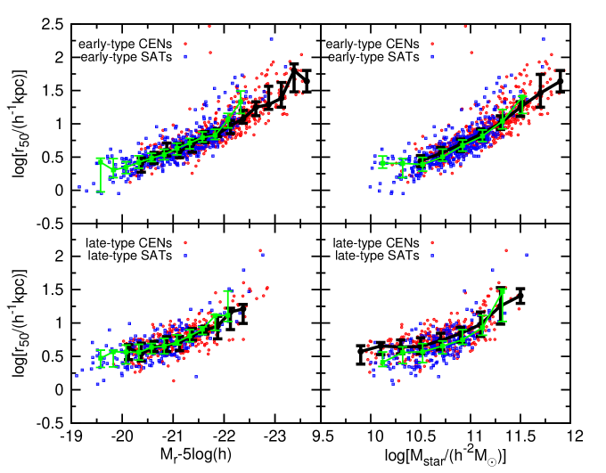
Figure 10: Comparison of CEN (red points) and SAT (blue points) galaxy size-luminosity (left column) and size-stellar mass (right column) scaling relations. These SATs (sample S1) have similar stellar masses as our CEN sample. The black (green) lines and errorbars show the median, first and third quartiles of the CEN (SAT) distribution in each luminosity or stellar mass bin. Both CENs and SATs are separated into early-type (upper panels) and late-type (lower panels) galaxies (see text for detail).

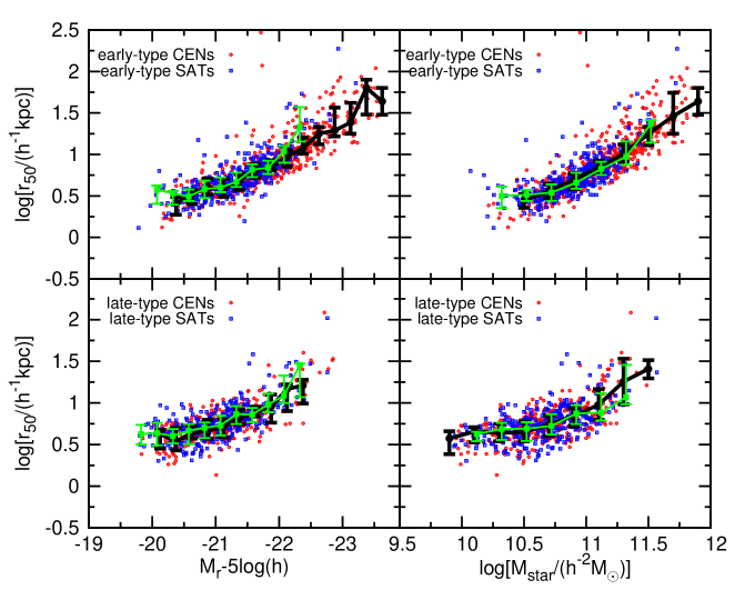
Figure 11: Same as Figure 10, except comparing CENs with SATs of similar stellar mass and colour.

Besides the $n$-${\rm M_{star}}$ relations, we use the $r_{50}$-$L$ and $r_{50}$-${\rm M_{star}}$ relations to compare the structural properties of CEN and SAT galaxies. We plot the sizes, luminosities, and stellar masses of our CEN sample from Figure 8 as red points in Figures 10 and Figure 11. The blue points represent the data for our SAT samples S1 (Fig. 10) and S2 (Fig. 11). The size, absolute magnitude and stellar mass of SATs are calculated in the same way as CENs as described in §4.1 and §4.2. Also, as in §4.2, we divide the SAT samples S1 and S2 into early-type and late-type galaxies based on our visual inspection. However, instead of computing the slopes of the CEN and SAT scaling relations, we compare the half-light size distributions (median, first, and third quartiles) of each sample in narrow bins of luminosity (0.25 mag wide for the $r_{50}$-$L$ relation) and stellar mass (0.2 dex wide for $r_{50}$-${\rm M_{star}}$ ). In this manner, we directly compare CENs with SATs from each sample only in regions of overlapping luminosity or stellar mass. Hence, we avoid comparing scaling relation slopes based upon samples that span different luminosity and stellar mass ranges. This helps to avoid the effects of small number statistics at the bright/massive and the faint/low-mass ends, which can bias the scaling relation slopes.

The comparisons in Figures 10 and 11 show that for early type galaxies, whether or not they are matched in colour, CENs and SATs display almost no difference in their size distributions. The only differences occur at the bright/massive ends of the SAT relations, where both SAT sample S1 and S2 suffer from small number statistics. For late-type SAT galaxies, the two samples also have size-luminosity relations that are similar to the CENs (the lower left panel in both figures). SATs have smaller median sizes than CENs when we only match in stellar mass (the lower right panel of Figure 10), but this difference disappears when we compare to SATs matched in both colour and stellar mass (the lower right panel of Figure 11).

4.3.3 Discussion

Using the $n$-${\rm M_{star}}$, $r_{50}$-$L$ and $r_{50}$-${\rm M_{star}}$ relations, we compare galaxies in our CEN sample to SATs of the same stellar mass. We find two basic differences between CEN and SAT galaxies: (1) low mass (${\rm log[M_{star}/(h^{-2}M_{\odot})]<10.75}$) SATs have a slightly higher median Sérsic index compared to CENs of the same stellar mass; and (2) low-mass, late-type SATs have smaller median sizes compared to their same-mass CEN counterparts. Our findings are in good qualitative agreement with the results of Weinmann et al. (2008) for a much larger SDSS sample. Using the NYU-VAGC half-light radii and concentrations for over $10^{5}$ galaxies, they found that late-type SATs are smaller and more concentrated than late-type CENs of the same stellar mass. We note, however, that their size measurements suffer from a systematic underestimate owing to an overestimate of the background sky levels (as we discuss in Appendix A).

We also find that the above two basic differences disappear when we compare CENs and SATs of the same stellar mass and optical colour. Moreover, we find no structural differences between high-mass (${\rm log[M_{star}/(h^{-2}M_{\odot})]>10.75}$) CEN and SAT galaxies, which tend to have early-type (spheroid-dominated) morphologies, or between early-type CENs and SATs, in general.

For lower-mass (${\rm log[M_{star}/(h^{-2}M_{\odot})]<10.75}$) SATs, the minor differences with CENs of similar stellar mass, and the lack of any difference with CENs of the same mass and colour, can be understood in terms of our selection criteria for the SAT sample S1 and S2. According to the hierarchical scenario of structure formation, larger haloes housing groups and clusters are formed through the accretion and merging of smaller haloes. Thus, all SATs were once the CEN galaxy in a smaller halo. Under this assumption, low-mass SATs tend to be redder on average than CENs of similar stellar mass because SATs have had their star formation quenched by environmental processes once they became non-CEN members of a larger halo (van den Bosch et al., 2008). In addition, as Weinmann et al. (2008) point out, quenching will also cause a moderate increase in the concentration and decrease in the size of late-type SATs, as we find here when comparing similar mass SATs and CENs. It is important to keep in mind that the average structural differences are small and, as such, SAT quenching cannot be used to explain the major morphological transformation of many disks into spheroids that is required to produce the strong morphological bimodality between blue and red galaxies. When we restrict our SAT selection to match lower-mass CENs in both stellar mass and colour (SAT sample S2), we preferentially choose blue SATs. Lower-mass CENs are typically blue (Figure 1) and their colour is associated with late-type morphology (disk-like) and on-going star formation. Therefore, we argue that blue SATs are likely examples of newly accreted SATs, i.e. recent CENs of the most recently accreted subhaloes. If true, new SATs have not been members of larger haloes long enough to alter their colour and structural properties. This line of reasoning agrees with the absence of structural differences we find for the CENs and SATs in SAT sample S2.

When we consider higher-mass (${\rm log[M_{star}/(h^{-2}M_{\odot})]>10.75}$) SATs (either sample S1 or S2), they have the same red colour (see lower left panel of Figure. 2) and highly-concentrated, large Sérsic index profiles associated with early-type morphologies as CENs of similar mass. While massive SATs are rare compared to their CEN counterparts, they are structurally indistinguishable. In a broader sense, we find that all morphologically early-type SATs and CENs have the same size scaling relations and that any reported differences between CENs and SATs (e.g. Graham et al., 1996; Liu et al., 2008) are actually the result of comparing two populations, e.g. BCGs and non-BCGs, with different stellar mass distributions. Owing to the similar red colours of massive CENs and SATs, there is no way to discern recent arrivals from long-term members in larger haloes, but it is clear that the transformation into spheroids does not depend on becoming a SAT. If that were true, we would expect massive CENs to be disk-like when they are clearly otherwise. Rather, we argue that the strong morphological transformation from disk to spheroid occurred at an earlier time when a massive SAT was the CEN of a smaller halo and that the local environment had no additional impact on the structure of high-mass spheroids. We find that the difference between disk-dominated and spheroid-dominated structure is more directly related to the stellar mass of a galaxy. Clearly, there is some relationship between the mass of CENs and their host halo mass (Figure 1), but further study is required to understand whether or not any aspect of the environment plays an important role in the transformation of disks and the production of high-mass spheroids.

5 Summary

In this paper, we study how the structural properties of central galaxies (CENs) in groups and clusters depend on galaxy stellar mass, global environment (group halo mass), and local environment (central/satellite position within the host halo). We select from the SDSS DR4 group catalogue (Yang et al., 2007) a statistically representative sample of 911 CENs whose host halo masses span from $10^{12}$ to ${\rm 10^{15}h^{-1}M_{\odot}}$. We use 2D Sérsic model fits to quantify the shape (Sérsic index) and size (half-light radius) of each galaxy. To this end, we establish a well-tested, GALFIT-based pipeline to fit Sérsic models to SDSS imaging data in the $r$-band. We summarise our main findings below.

We thoroughly test the performance of our GALFIT pipeline on simulated and real SDSS galaxy image data. Our 2D fitting recovers the structural properties of simulated galaxies with no bias, unlike the one-dimensional fits to azimuthally-averaged data employed for the NYU-VAGC that systematically underestimate the total flux, size and Sérsic index of higher-$n$ profiles. For galaxy profile fitting, we also demonstrate that the SDSS global sky is preferred over the SDSS local value as a background level measurement. We compare our fitting results with those from the NYU-VAGC and find that our fits include light from the outer parts of galaxies, which is missed when an overestimate of the (local) sky background is used. We test how this background uncertainty translates into a systematic uncertainty in the fitting parameters owing to a strong covariance between Sérsic index, total magnitude, and half-light size. This covariance affects bright and large galaxies more and could contribute to the apparent steeping in the slope of the size-luminosity and size-stellar mass relations at the bright (massive) end.

We find that the Sérsic index of CENs depends strongly on ${\rm M_{star}}$, but weakly or not at all on ${\rm M_{halo}}$. The dependence on stellar mass is in the sense that low mass galaxies (${\rm M_{star}<10^{10.5}h^{-2}M_{\odot}}$) have lower, disk-like indices ($n\sim 2.0$), while massive galaxies (${\rm M_{star}>10^{11.0}h^{-2}M_{\odot}}$) have higher, spheroid-like ($\sim 5$) indices. Over a large range in ${\rm M_{halo}}$ , from small groups to large clusters, any change in the $n$ distribution of CENs is likely the result of the correlation between ${\rm M_{star}}$ and ${\rm M_{halo}}$. The fact that spheroidal CENs are found at all group masses, and the lack of a strong $n$ dependence on ${\rm M_{halo}}$ , both rule out a distinct halo mass for producing spheroids. Moreover, the strong dependence of $n$ on ${\rm M_{star}}$ suggests that ${\rm M_{star}}$ is the key factor in determining the shape of CENs.

Similar to the light profile shape, the half-light size of CENs depends on galaxy stellar mass and luminosity. We separate our CEN sample into early and late-type galaxies by visual inspection and we find a $r_{50}$-$L$ slope of $\alpha\sim 0.83(0.62)$ for early-type (late-type) galaxies with $-22<{\rm M_{r}-5log(h)}<-20$. We also compare our $r_{50}$-$L$ slope for early-type CENs with those from other studies and find that there is fairly large discrepancy. This discrepancy could result from several factors including different samples, size measurement techniques, or early-type galaxy definitions.

To study whether the structural properties of CENs depend on their special position at the centre of the gravitational potential well, we compare their shapes and sizes with those of non-CEN satellite (SAT) galaxies. We find that low mass ($<10.0^{10.75}{\rm h^{-2}M_{\odot}}$) SATs have somewhat larger median Sérsic indices compared with CENs of similar stellar mass. In addition, low mass late-type SATs are moderately smaller in size than late-type CENs when matched in stellar mass, but no size differences are found between early-type CENs and SATs. We find no structural differences between SATs and CENs when they are matched in both optical colour and stellar mass. The small differences in the sizes of low-mass, late-type CENs and SATs are consistent with SAT quenching as found by others (e.g., in van den Bosch et al. (2008) and Weinmann et al. (2008)). The similarity in the structure of massive SATs and massive CENs demonstrates that the local environment has no significant impact on the structure of a massive galaxy that enters a denser environment and that these two populations are morphologically indistinguishable.

We conclude that ${\rm M_{star}}$ is the most fundamental property in determining the basic structural shape and size of a galaxy. In contrast, the lack of a significant $n$-${\rm M_{halo}}$ relation rules out a clear distinct group mass for producing spheroids. This fact, combined with the existence of spheroid CENs in low-mass and high-mass groups, suggests that the strong morphological transformation processes that produce spheroids must occur at the centres of groups spanning a wide range of masses.

Appendix A Comparison with NYU-VAGC Sérsic Fits

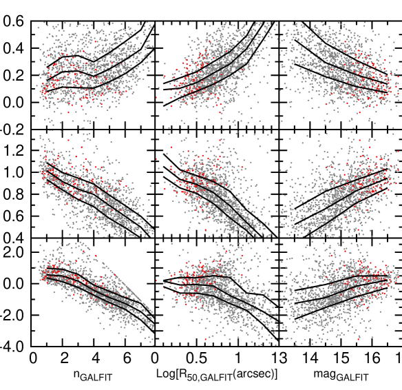
Figure 12: Differences between the NYU-VAGC and GALFIT Sérsic parameters from $r$-band SDSS data as a function of the GALFIT Sérsic parameters for our total sample of 1657 CEN+SAT galaxies. The lines show the quartiles of each distribution as in Fig. 3. Black points are for galaxies with $|\mathrm{\Delta sky|>0.1\ ADU}$ and red points for $|\mathrm{\Delta sky|<0.1\ ADU}$, where $\mathrm{\Delta sky=local\ sky-global\ sky}$. Note, in the left panels it is clear that the NYU-VAGC fitting has an $n=6$ limit.

Blanton et al. (2005, hereafter ’NYU-VAGC’) fit Sérsic models to the azimuthally-averaged 1D profiles output by the SDSS photometric pipeline (Stoughton et al., 2002) for all SDSS DR4 galaxies meeting the Main sample criteria. Tests show that the NYU-VAGC Sérsic fitting does well for simulated galaxies with an input Sérsic index $n_{\rm in}<2$, a small size or a faint magnitude. But for $n_{\rm in}>2$ simulations, the NYU-VAGC fitting systematically underestimates $n$, $r_{50}$, and total flux [see Figure 9 in Blanton et al. (2005) for details]. For example, for a simulated galaxy with $n_{in}=4$ the NYU-VAGC fitting underestimates these parameters by 15 percent. For comparison, our GALFIT fitting results for 850 simulated Sérsic galaxies placed in SDSS images show very little bias for $n_{in}>4$ galaxies (see Figure 3). Note that we adopt the global sky value from the SDSS image header in our GALFIT profile fits, while NYU-VAGC uses the local sky level. It has been reported that the SDSS pipeline overestimates the local sky in dense environments (Lauer et al., 2007; von der Linden et al., 2007; Adelman-McCarthy et al., 2008). As such, Sérsic fits based on overestimates of the sky may result in fainter magnitudes, smaller sizes and/or lower Sérsic indices as we demonstrate in §3.4.

Figure 12 shows comparisons between our fit results and those from NYU-VAGC for our total sample of 911 CENs plus 746 SATs from our SAT sample S2 (see §2 for details). Below, we discuss in detail the discrepancies between the two fits for galaxies with $n>3$ from GALFIT, and then for those with lower Sérsic indices.

A.1 High Sérsic Galaxies

For $n>3$ galaxies, the NYU-GALFIT parameter discrepancy for real galaxies in Figure 12 follows a similar trend as those between the input and fit parameters for simulated galaxies in Figure 9 of Blanton et al. (2005), but with an increased amplitude. For example, the Sérsic difference (lower left panel) grows by about $\Delta n\simeq 1.3$ over the interval $3<n<6$, compared with $\Delta n\simeq 0.6$ over the same interval in the Blanton et al. (2005) simulations. Here two factors are at play: one is the systematic underestimate of NYU-VAGC’s 1D fitting procedure for steep Sérsic profiles as demonstrated in their test fitting using simulations. The second factor is the difference between the sky levels used in each procedure. In Figure 13, we attempt to separate these two factors by splitting the whole sample into GALFIT Sérsic index and relative sky difference bins, where the relative sky difference is the difference between the local and the global sky normalised by the Petrosian surface brightness of the galaxies ($I_{petro}=f_{Petro}/(2\pi r^{2}_{50,Petro})$ in units of ADUs per pixel, where $f_{Petro}$ and $r_{50,Petro}$ are the Petrosian flux and Petrosian half-light radius, respectively). For $n>4$ galaxies with a normalised sky difference less than 0.01, meaning that the sky difference is at most a minor issue, the $n$ and $r_{50}$ disagreements more or less reflect the systematic underestimates seen in the NYU-VAGC fitting of simulated galaxies. As $\Delta sky/I_{petro}$ increases, the NYU-GALFIT disagreements grow and we see a trend of larger NYU-VAGC underestimates for galaxies with higher $n$, as expected when the local sky estimate includes more of the light belonging to each galaxy.

A.2 Low Sérsic Galaxies

We have outlined how the NYU-VAGC and GALFIT methods both do very well in fitting pure-Sérsic simulations with $n_{\rm in}<3$, therefore we expect minor differences when comparing fits to real galaxies with disk-like profiles. However, we find that the fit parameters from the two procedures differ in two ways for $n<3$ galaxies, as shown in Figure 12. First, the NYU-VAGC fits have systematically higher Sérsic values than the GALFIT fits, which is inconsistent with the results from the simulations. Second, there is a systematic offset of about 0.2 mag between the magnitude of NYU-VAGC fits and our GALFIT fits in the sense that NYU-VAGC finds fainter fluxes. We note that the offset appears to be independent of the difference in the sky ($\mathrm{\Delta sky=local\ sky\ -\ global\ sky}$) used in each fitting procedure, as shown by the similarity between the red (small $\mathrm{\Delta sky}$) and the black (large $\mathrm{\Delta sky}$) points for $n<3$ galaxies in Figure 12.

We suspect that the NYU-VAGC procedure of fitting a 1-D Sérsic model to azimuthally averaged annuli overestimates Sérsic indices for disk galaxies. We check the distribution of Sérsic indices for the whole NYU-VAGC and find that the number of galaxies with $0.5<n_{\rm NYU-VAGC}<1.0$ is much less than those with $1.0<n_{\rm NYU-VAGC}<1.5$. This results in conflicts with other observations of disk galaxies (e.g. Driver et al., 2006; van der Wel, 2008; Häussler et al., 2007). To test our suspicion, we visually inspect galaxies from our sample with a late-type fit ($n<2$) by GALFIT, but an early-type fit ($n_{\rm NYU-VAGC}>2.5$) by NYU-VAGC. To exclude the sky influence, we restrict our inspection to 36 galaxies with $|\Delta{\rm sky}|<0.5{\rm\ ADU}$. At least two thirds of these galaxies have very obvious spiral features as expected for galaxies with disk-dominated light profiles. Another 20 percent have disturbed morphologies or very bright nearby stars, which could cause spurious fits. A majority of the spirals are inclined with $b/a<0.5$. As clearly demonstrated by Bailin & Harris (2008), $n_{NYU-VAGC}$ is systematically overestimated for more inclined galaxies. This effect is the result of edge-on or inclined galaxies having steeper azimuthally averaged radial profiles because the averaged flux from the narrow outer part of such galaxy is decreased by being smoothed over a large circular area.

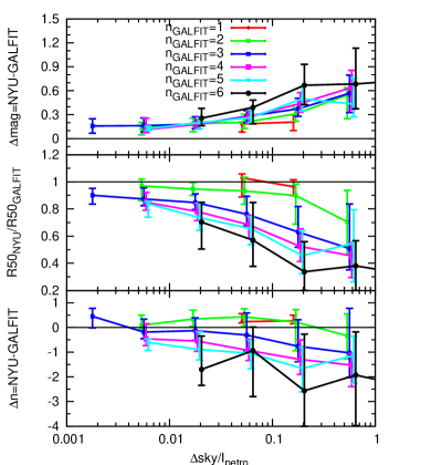
Figure 13: The NYU-GALFIT discrepancies shown in Figure 12 as a function of sky difference, divided into GALFIT Sérsic index bins as shown by the colour coding. Here the sky difference is expressed by the ratio between $\mathrm{\Delta sky=local\ sky-global\ sky}$ and the average Petrosian surface brightness (Petrosian quantities are directly drawn from SDSS tables).

A.3 Comparing Sérsic Magnitude Estimates

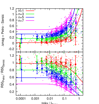
Figure 14: The difference between Petrosian and Sérsic model quantities as a function of sky offset normalised to the Petrosian surface brightness. Cases with different Sérsic index are colour coded as indicated in the top panel. Solid lines are for our predictions based on a pure Sérsic model (see text for details), for which $\Delta{\rm sky}$ means the imaginary overestimation of sky background. The small squares are for each galaxy in our GALFIT sample, for which $\Delta{\rm sky}$ means the SDSS local-global sky difference. The filled circles with error bars show the mean and standard deviation of our sample in different bins. We also compare with the mean and standard deviation (triangles with error bars) of the NYU-VAGC fitting parameters, which should be plotted at $\mathrm{\Delta sky=0}$, but are shifted a little to allow them to be plotted on a log-scale plot.

Besides the tendency to overestimate the Sérsic indices of actual disk-dominated galaxies when using 1D fits to azimuthally-averaged radial profiles, we also explore the offset between the NYU-VAGC and the GALFIT Sérsic magnitudes in more detail. For this exercise we use an independent measure of galaxy flux, the SDSS Petrosian magnitude, to anchor our comparisons of different Sérsic magnitudes from the two methods. The SDSS photometric pipeline calculates the flux within a circular aperture equal to two times the Petrosian radius, which provides an approximate total galaxy magnitude. It is well known, however, that Petrosian magnitudes systematically miss some flux when applied to different Sérsic model profiles. As shown in Graham et al. (2005), the Petrosian magnitude misses very little flux for an $n=1$ profile, but for an $n=4$ galaxy it will underestimate the brightness by about 0.2 magnitudes. We note that the Graham et al. (2005) calculations are valid only when the sky is known perfectly. Any under/overestimation of the sky background will increase/decrease the discrepancy between the Petrosian and the Sérsic magnitudes. Using the formalism of Graham et al. (2005), we predict the Petrosian-Sérsic magnitude offset ($\Delta{\rm mag}={\rm Petrosian-Sersic}$) under the influence of different amounts of overestimation of the real sky by subtracting a range of background pedestals to each Sérsic model before measuring the Petrosian flux. Our $\Delta{\rm mag}$ predictions for different $n$ are shown in Figure 14 (top panel) as a function of the sky overestimate ($\Delta{\rm sky}$), normalised by the Petrosian surface brightness (as in Figure 13). When the normalised sky difference is less than $10^{-4}$, our predictions converge as expected to the values claimed in Graham et al. (2005). However, as the overestimates of the local sky increase, underestimates of the Petrosian magnitude for different $n$ grow systematically. Likewise, we also make predictions for the offsets between the Petrosian and the Sérsic half-light radii ($r_{50,{\rm Petro}}/r_{50,{\rm Sersic}}$) as a function of sky offsets and plot these in the bottom panel of Figure 14.

In Figure 14, we also compare our GALFIT results for actual galaxies (small squares) to the sky dependent predictions. Our working assumptions are: (1) a Sérsic model is a reasonable model to describe galaxy light profiles, and (2) the SDSS global sky is a good measurement of the real sky and is preferred to using the SDSS local value. Here $\Delta{\rm sky}$ is the local-global sky difference in SDSS and all the Petrosian results are measured using the local sky. In the upper panel, we see that our fit results are close to the $\Delta{\rm mag}$ predictions for a wide range of sky differences and Sérsic indices. We also find fair agreement between our $r_{50}$ results and the predictions in the lower panel of Figure 14, suggesting that our fitting results are self-consistent under the two assumptions above.

Finally, we compare the NYU-VAGC results for the real data with the predictions. Given that the NYU-VAGC fitting uses the same local sky as the Petrosian quantities, all the galaxies with NYU-VAGC fits have $\Delta{\rm sky}=0$ by definition. Therefore, the values of $\Delta{\rm mag}$ and $r_{50,{\rm Petro}}/r_{50,{\rm Sersic}}$ for the NYU-VAGC Sérsic results for our sample (triangles in Figure 14) should satisfy the predictions of Graham et al. (2005). Yet, we see that the NYU-VAGC Sérsic results are actually underestimates, on average, compared to the predictions. For example, the $n=1$ galaxies have Sérsic magnitudes that are 0.1 mag fainter than the Petrosian measurement, which is inconsistent with either the predictions or the definition of the two magnitudes. By definition, Sérsic magnitudes are based on a model flux integrated to infinity, thus there is no reason for such a magnitude to be fainter than the Petrosian aperture magnitude, which only includes light our to some radius. It is unclear why the NYU-VAGC Sérsic fitting procedure produces fainter magnitudes than expected, but this effect combined with the nonzero $\Delta{\rm sky}$ values explain the systematic 0.2 mag offset that we find between the GALFIT and the NYU-VAGC Sérsic magnitudes for $n<3$ galaxies (Figure 12). Based on the above analysis, we conclude that if the two assumptions of our fitting are valid, i.e. assuming a Sérsic model is the correct model and that the SDSS global sky is an accurate measure of the true sky background, then our GALFIT fitting of the SDSS data returns more accurate measurements for the structural parameters of galaxies than those in the NYU-VAGC.

References

- Aceves et al. (2006) Aceves H., Velázquez H., Cruz F., 2006, MNRAS, 373, 632
- Adelman-McCarthy et al. (2008) Adelman-McCarthy J. K. et al. 2008, ApJS, 175, 297
- Adelman-McCarthy et al. (2006) Adelman-McCarthy J. K. et al. 2006, ApJS, 162, 38
- Allen et al. (2006) Allen P. D., Driver S. P., Graham A. W., Cameron E., Liske J., de Propris R., 2006, MNRAS, 371, 2
- Bailin & Harris (2008) Bailin J., Harris W. E., 2008, MNRAS, 385, 1835
- Balogh et al. (2004) Balogh M. et al. 2004, MNRAS, 348, 1355
- Barnes & Hernquist (1996) Barnes J. E., Hernquist L., 1996, ApJ, 471, 115
- Bell et al. (2003) Bell E. F., McIntosh D. H., Katz N., Weinberg M. D., 2003, ApJS, 149, 289
- Bell et al. (2004) Bell E. F. et al. 2004, ApJ, 608, 752
- Bernardi et al. (2007) Bernardi M., Hyde J. B., Sheth R. K., Miller C. J., Nichol R. C., 2007, AJ, 133, 1741
- Bertin & Arnouts (1996) Bertin E., Arnouts S., 1996, A&AS, 117, 393
- Blanton (2006) Blanton M. R., 2006, ApJ, 648, 268
- Blanton et al. (2003) Blanton M. R. et al. 2003, AJ, 125, 2348
- Blanton et al. (2005) Blanton M. R., Eisenstein D., Hogg D. W., Schlegel D. J., Brinkmann J., 2005, ApJ, 629, 143
- Blanton et al. (2003) Blanton M. R. et al. 2003, ApJ, 594, 186
- Blanton et al. (2005) Blanton M. R. et al. 2005, AJ, 129, 2562
- Borch et al. (2006) Borch A. et al. 2006, A&A, 453, 869
- Brown et al. (2007) Brown M. J. I., Dey A., Jannuzi B. T., Brand K., Benson A. J., Brodwin M., Croton D. J., Eisenhardt P. R., 2007, ApJ, 654, 858
- Byun & Freeman (1995) Byun Y. I., Freeman K. C., 1995, ApJ, 448, 563
- Cavaliere et al. (1992) Cavaliere A., Colafrancesco S., Menci N., 1992, ApJ, 392, 41
- Colless et al. (2001) Colless M. et al. 2001, MNRAS, 328, 1039
- Cooray & Milosavljević (2005) Cooray A., Milosavljević M., 2005, ApJL, 627, L85
- Cox et al. (2006) Cox T. J., Dutta S. N., Di Matteo T., Hernquist L., Hopkins P. F., Robertson B., Springel V., 2006, ApJ, 650, 791
- de Jong (1996) de Jong R. S., 1996, A&AS, 118, 557
- de Jong et al. (2004) de Jong R. S., Simard L., Davies R. L., Saglia R. P., Burstein D., Colless M., McMahan R., Wegner G., 2004, MNRAS, 355, 1155
- Desroches et al. (2007) Desroches L.-B., Quataert E., Ma C.-P., West A. A., 2007, MNRAS, 377, 402
- Dressler (1980) Dressler A., 1980, ApJ, 236, 351
- Driver et al. (2006) Driver S. P. et al. 2006, MNRAS, 368, 414
- Dutton et al. (2007) Dutton A. A., van den Bosch F. C., Dekel A., Courteau S., 2007, ApJ, 654, 27
- Faber et al. (2007) Faber S. M., Willmer C. N. A., Wolf C., Koo D. C., Weiner B. J., et al. 2007, ApJ, 665, 265
- Gonzalez et al. (2005) Gonzalez A. H., Zabludoff A. I., Zaritsky D., 2005, ApJ, 618, 195
- Goto et al. (2003) Goto T., Yamauchi C., Fujita Y., Okamura S., Sekiguchi M., Smail I., Bernardi M., Gomez P. L., 2003, MNRAS, 346, 601
- Graham et al. (1996) Graham A., Lauer T. R., Colless M., Postman M., 1996, ApJ, 465, 534
- Graham et al. (2005) Graham A. W., Driver S. P., Petrosian V., Conselice C. J., Bershady M. A., Crawford S. M., Goto T., 2005, AJ, 130, 1535
- Hashimoto et al. (1998) Hashimoto Y., Oemler A. J., Lin H., Tucker D. L., 1998, ApJ, 499, 589
- Häussler et al. (2007) Häussler B. et al. 2007, ApJS, 172, 615
- Hogg et al. (2004) Hogg D. W. et al. 2004, ApJL, 601, L29
- Hopkins et al. (2008) Hopkins P. F., Hernquist L., Cox T. J., Kereš D., 2008, ApJS, 175, 356
- Kauffmann et al. (2004) Kauffmann G., White S. D. M., Heckman T. M., Ménard B., Brinchmann J., Charlot S., Tremonti C., Brinkmann J., 2004, MNRAS, 353, 713
- Khosroshahi et al. (2000) Khosroshahi H. G., Wadadekar Y., Kembhavi A., 2000, ApJ, 533, 162
- Kroupa (2001) Kroupa P., 2001, MNRAS, 322, 231
- Lauer et al. (2007) Lauer T. R. et al. 2007, ApJ, 662, 808
- Liu et al. (2008) Liu F. S., Xia X. Y., Mao S., Wu H., Deng Z. G., 2008, MNRAS, 385, 23
- MacArthur et al. (2003) MacArthur L. A., Courteau S., Holtzman J. A., 2003, ApJ, 582, 689
- Maller et al. (2008) Maller A. H., Berlind A. A., Blanton M. R., Hogg D. W., 2008, ArXiv e-prints, 801
- McIntosh et al. (2008) McIntosh D. H., Guo Y., Hertzberg J., Katz N., Mo H. J., van den Bosch F. C., Yang X., 2008, MNRAS, 388, 1537
- McIntosh et al. (2004) McIntosh D. H., Rix H.-W., Caldwell N., 2004, ApJ, 610, 161
- Miller et al. (2005) Miller C. J. et al. 2005, AJ, 130, 968
- Moore et al. (1996) Moore B., Katz N., Lake G., Dressler A., Oemler A., 1996, Nature, 379, 613
- Naab & Burkert (2003) Naab T., Burkert A., 2003, ApJ, 597, 893
- Naab & Trujillo (2006) Naab T., Trujillo I., 2006, MNRAS, 369, 625
- Peng et al. (2002) Peng C. Y., Ho L. C., Impey C. D., Rix H.-W., 2002, AJ, 124, 266
- Schlegel et al. (1998) Schlegel D. J., Finkbeiner D. P., Davis M., 1998, ApJ, 500, 525
- Sérsic (1968) Sérsic J. L., 1968, Atlas de galaxias australes. Cordoba, Argentina: Observatorio Astronomico, 1968
- Shaw & Gilmore (1989) Shaw M. A., Gilmore G., 1989, MNRAS, 237, 903
- Shen et al. (2003) Shen S., Mo H. J., White S. D. M., Blanton M. R., Kauffmann G., Voges W., Brinkmann J., Csabai I., 2003, MNRAS, 343, 978 (S03)
- Simard (1998) Simard L., 1998, in Albrecht R., Hook R. N., Bushouse H. A., eds, Astronomical Data Analysis Software and Systems VII Vol. 145 of Astronomical Society of the Pacific Conference Series, GIM2D: an IRAF package for the Quantitative Morphology Analysis of Distant Galaxies. p. 108
- Stoughton et al. (2002) Stoughton C. et al. 2002, AJ, 123, 485
- Strauss et al. (2002) Strauss M. A. et al. 2002, AJ, 124, 1810
- Toomre (1977) Toomre A., 1977, in Evolution of Galaxies and Stellar Populations Mergers and Some Consequences. p. 401
- van den Bosch et al. (2008) van den Bosch F. C., Aquino D., Yang X., Mo H. J., Pasquali A., McIntosh D. H., Weinmann S. M., Kang X., 2008, MNRAS, 387, 79
- van der Wel (2008) van der Wel A., 2008, ApJL, 675, L13
- von der Linden et al. (2007) von der Linden A., Best P. N., Kauffmann G., White S. D. M., 2007, MNRAS, 379, 867
- Weinmann et al. (2008) Weinmann S. M., Kauffmann G., van den Bosch F. C., Pasquali A., McIntosh D. H., Mo H., Yang X., Guo Y., 2008, ArXiv e-prints
- Weinmann et al. (2006) Weinmann S. M., van den Bosch F. C., Yang X., Mo H. J., 2006, MNRAS, 366, 2
- Yang et al. (2005) Yang X., Mo H. J., van den Bosch F. C., Jing Y. P., 2005, MNRAS, 356, 1293
- Yang et al. (2007) Yang X., Mo H. J., van den Bosch F. C., Pasquali A., Li C., Barden M., 2007, ApJ, 671, 153 (Y07)
- York et al. (2000) York D. G. et al. 2000, AJ, 120, 1579