Improved Measurement of Absolute Branching Fraction of $\bm{D^{+}_{s}\rightarrow\tau^{+}\nu_{\tau}}$

Abstract

We have studied the leptonic decay $D^{+}_{s}\to\tau^{+}\nu_{\tau}$, via the decay channel $\tau^{+}\to e^{+}\nu_{e}\bar{\nu}_{\tau}$, using a sample of tagged $D_{s}^{+}$ decays collected near the $D^{\ast\pm}_{s}D^{\mp}_{s}$ peak production energy in $e^{+}e^{-}$ collisions with the CLEO-c detector. We obtain $\mathcal{B}(D^{+}_{s}\to\tau^{+}\nu_{\tau})=(5.30\pm 0.47\pm 0.22)\%$ and determine the decay constant $f_{D_{s}}=(252.5\pm 11.1\pm 5.2)$ MeV, where the first uncertainties are statistical and the second are systematic.

I Introduction

The leptonic decays of a charged pseudoscalar meson $P^{+}$ are processes of the type $P^{+}\to\ell^{+}\nu_{\ell}$, where $\ell=e$, $\mu$, or $\tau$. Because no strong interactions are present in the leptonic final state $\ell^{+}\nu_{\ell}$, such decays provide a clean way to probe the complex, strong interactions that bind the quark and antiquark within the initial-state meson. In these decays, strong interaction effects can be parametrized by a single quantity, $f_{P}$, the pseudoscalar meson decay constant. The leptonic decay rate can be measured by experiment, and the decay constant can be determined by the equation (ignoring radiative corrections)

$$\Gamma(P_{Q\bar{q}}\rightarrow\ell^{+}\nu_{\ell})=\frac{G^{2}_{F}|V_{Qq}|^{2}f^{2}_{P}}{8\pi}m_{P}m^{2}_{\ell}\left(1-\frac{m^{2}_{\ell}}{m^{2}_{P}}\right)^{2},$$ (1)

where $G_{F}$ is the Fermi coupling constant, $V_{Qq}$ is the Cabibbo-Kobayashi-Maskawa (CKM) matrix Cabibbo:1963yz ; Kobayashi:1973fv element, $m_{P}$ is the mass of the meson, and $m_{\ell}$ is the mass of the charged lepton. The quantity $f_{P}$ describes the amplitude for the $Q$ and $\bar{q}$-quarks within the $P$ to have zero separation, a condition necessary for them to annihilate into the virtual $W^{+}$ boson that produces the $\ell^{+}\nu_{\ell}$ pair.

The experimental determination of decay constants is one of the most important tests of calculations involving nonperturbative QCD. Such calculations have been performed using various models Amsler:2008zz or using lattice QCD (LQCD). The latter is now generally considered to be the most reliable way to calculate the quantity.

Knowledge of decay constants is important for describing several key processes, such as $B-\bar{B}$ mixing, which depends on $f_{B}$, a quantity that is also predicted by LQCD calculations. Experimental determination Ikado:2006un ; Aubert:2007xj of $f_{B}$ with the leptonic decay of a $B^{+}$ meson is, however, very limited as the rate is highly suppressed due to the smallness of the magnitude of the relevant CKM matrix element $V_{ub}$. The charm mesons, $D^{+}$ and $D^{+}_{s}$, are better instruments to study the leptonic decays of heavy mesons since these decays are either less CKM suppressed or favored, i.e., $\Gamma(D^{+}\to\ell^{+}\nu_{\ell})\propto|V_{cd}|^{2}\approx(0.23)^{2}$ and $\Gamma(D^{+}_{s}\to\ell^{+}\nu_{\ell})\propto|V_{cs}|^{2}\approx(0.97)^{2}$ are much larger than $\Gamma(B^{+}\to\ell^{+}\nu_{\ell})\propto|V_{ub}|^{2}\approx(0.004)^{2}$. Thus, the decay constants $f_{D}$ and $f_{D_{s}}$ determined from charm meson decays can be used to test and validate the necessary LQCD calculations applicable to the $B$-meson sector.

Among the leptonic decays in the charm-quark sector, $D^{+}_{s}\to\ell^{+}\nu_{\ell}$ decays are more accessible since they are CKM favored. Furthermore, the large mass of the $\tau$ lepton removes the helicity suppression that is present in the decays to lighter leptons. The existence of multiple neutrinos in the final state, however, makes measurement of this decay challenging.

Physics beyond the standard model (SM) might also affect leptonic decays of charmed mesons. Depending on the non-SM features, the ratio of $\Gamma(D^{+}\to\ell^{+}\nu_{\ell})/\Gamma(D^{+}_{s}\to\ell^{+}\nu_{\ell})$ could be affected Akeroyd:2007eh , as could the ratio Hewett:1995aw ; Hou:1992sy $\Gamma(D^{+}_{s}\to\tau^{+}\nu_{\tau})/\Gamma(D^{+}_{s}\to\mu^{+}\nu_{\mu})$. Any of the individual widths might be increased or decreased. There is an indication of a discrepancy between the experimental determinations Amsler:2008zz of $f_{D_{s}}$ and the most recent precision LQCD calculation Follana:2007uv . This disagreement is particularly puzzling since the CLEO-c determination :2008sq of $f_{D}$ agrees well with the LQCD calculation Follana:2007uv of that quantity. Some Dobrescu:2008er conjecture that this discrepancy may be explained by a charged Higgs boson or a leptoquark.

In this article, we report an improved measurement of the absolute branching fraction of the leptonic decay $D^{+}_{s}\to\tau^{+}\nu_{\tau}$ (charge-conjugate modes are implied), with $\tau^{+}\to e^{+}\nu_{e}\bar{\nu}_{\tau}$, from which we determine the decay constant $f_{D_{s}}$.

II Data and The CLEO-c Detector

We use a data sample of $e^{+}e^{-}\to D^{\ast\pm}_{s}D^{\mp}_{s}$ events provided by the Cornell Electron Storage Ring (CESR) and collected by the CLEO-c detector at the center-of-mass (CM) energy $4170$ MeV, near $D^{\ast\pm}_{s}D^{\mp}_{s}$ peak production CroninHennessy:2008yi . The data sample consists of an integrated luminosity of $602$ $\text{pb}^{-1}$ containing $5.5\times 10^{5}$ $D^{\ast\pm}_{s}D^{\mp}_{s}$ pairs. We have previously reported Artuso:2007zg ; :2007zm measurements of $D^{+}_{s}\to\mu^{+}\nu_{\mu}$ and $D^{+}_{s}\to\tau^{+}\nu_{\tau}$ with a subsample of these data. A companion article Syracuse:2008new reports measurements of $f_{D_{s}}$ from $D^{+}_{s}\to\mu^{+}\nu_{\mu}$ and $D^{+}_{s}\to\tau^{+}\nu_{\tau}$, with $\tau^{+}\to\pi^{+}\bar{\nu}_{\tau}$, using essentially the same data sample as the one used in this measurement.

The CLEO-c detector Briere:2001rn ; Kubota:1991ww ; cleoiiidr ; cleorich is a general-purpose solenoidal detector with four concentric components utilized in this measurement: a small-radius six-layer stereo wire drift chamber, a 47-layer main drift chamber, a Ring-Imaging Cherenkov (RICH) detector, and an electromagnetic calorimeter consisting of 7800 CsI(Tl) crystals. The two drift chambers operate in a $1.0$ T magnetic field and provide charged particle tracking in a solid angle of $93$% of $4\pi$. The chambers achieve a momentum resolution of $\sim 0.6$% at $p=1$ GeV/$c$. The main drift chamber also provides specific-ionization ($dE/dx$) measurements that discriminate between charged pions and kaons. The RICH detector covers approximately $80$% of $4\pi$ and provides additional separation of pions and kaons at high momentum. The photon energy resolution of the calorimeter is $2.2$% at $E_{\gamma}=1$ GeV and $5$% at $100$ MeV. Electron identification is based on a likelihood variable that combines the information from the RICH detector, $dE/dx$, and the ratio of electromagnetic shower energy to track momentum ($E/p$).

We use a GEANT-based geant Monte Carlo (MC) simulation program to study efficiency of signal-event selection and background processes. Physics events are generated by evtgen evtgen , tuned with much improved knowledge of charm decays :2007zt ; :2008cqa , and final-state radiation (FSR) is modeled by the photos photos program. The modeling of initial-state radiation (ISR) is based on cross sections for $D^{\ast\pm}_{s}D^{\mp}_{s}$ production at lower energies obtained from the CLEO-c energy scan CroninHennessy:2008yi near the CM energy where we collect the sample.

III Analysis Method

The presence of two $D^{\mp}_{s}$ mesons in a $D^{\ast\pm}_{s}D^{\mp}_{s}$ event allows us to define a single-tag (ST) sample in which a $D^{\mp}_{s}$ is reconstructed in a hadronic decay mode and a further double-tagged (DT) subsample in which an additional $e^{\pm}$ is required as a signature of $\tau^{\pm}$ decay, the $e^{\pm}$ being the daughter of the $\tau^{\pm}$. The $D^{-}_{s}$ reconstructed in the ST sample can be either primary or secondary from $D^{\ast-}_{s}\to D^{-}_{s}\gamma$ (or $D^{\ast-}_{s}\to\pi^{0}D^{-}_{s}$). The ST yield can be expressed as

$$n_{\text{ST}}=2N\mathcal{B}_{\text{ST}}\epsilon_{\text{ST}},$$ (2)

where $N$ is the produced number of $D^{\ast\pm}_{s}D^{\mp}_{s}$ pairs, $\mathcal{B}_{\text{ST}}$ is the branching fraction of hadronic modes used in the ST sample, and $\epsilon_{\text{ST}}$ is the ST efficiency. The $n_{\text{ST}}$ counts the candidates, not events, and the factor of 2 comes from the sum of $D^{+}_{s}$ and $D^{-}_{s}$ tags.

Our double-tag (DT) sample is formed from events with only a single charged track, identified as an $e^{+}$, in addition to a ST. The yield can be expressed as

$$n_{\text{DT}}=2N\mathcal{B}_{\text{ST}}\mathcal{B}_{\text{L}}\epsilon_{\text{DT}},$$ (3)

where $\mathcal{B}_{\text{L}}$ is the leptonic decay branching fraction, including the subbranching fraction of $\tau^{+}\to e^{+}\nu_{e}\bar{\nu}_{\tau}$ decay, $\epsilon_{\text{DT}}$ is the efficiency of finding the ST and the leptonic decay in the same event. From the ST and DT yields we can obtain an absolute branching fraction of the leptonic decay $\mathcal{B}_{\text{L}}$, without needing to know the integrated luminosity or the produced number of $D^{\ast\pm}_{s}D^{\mp}_{s}$ pairs,

$$\mathcal{B}_{\text{L}}=\frac{n_{\text{DT}}}{n_{\text{ST}}}\frac{\epsilon_{\text{ST}}}{\epsilon_{\text{DT}}}=\frac{n_{\text{DT}}/\epsilon}{n_{\text{ST}}},$$ (4)

where $\epsilon$ ($\equiv\epsilon_{\text{DT}}/\epsilon_{\text{ST}}$) is the effective signal efficiency. Because of the large solid angle acceptance with high segmentation of the CLEO-c detector and the low multiplicity of the events with which we are concerned, $\epsilon_{\text{DT}}\approx\epsilon_{\text{ST}}\epsilon_{\text{L}}$, where $\epsilon_{\text{L}}$ is the leptonic decay efficiency. Hence, the ratio $\epsilon_{\text{DT}}/\epsilon_{\text{ST}}$ is insensitive to most systematic effects associated with the ST, and the signal branching fraction $\mathcal{B}_{\text{L}}$ obtained using this procedure is nearly independent of the efficiency of the tagging mode.

III.1 Event and tag selection

To minimize systematic uncertainties, we tag using three two-body hadronic decay modes with only charged particles in the final state. The three ST modes are $D^{-}_{s}\to\phi\pi^{-}$, $D^{-}_{s}\to K^{-}K^{\ast 0}$, and $D_{s}^{-}\to K^{0}_{S}K^{-}$. Using these tag modes also helps to reduce the tag bias which would be caused by the correlation between the tag side and the signal side reconstruction if tag modes with high multiplicity and large background were used. The effect of the tag bias $b_{\text{tag}}$ can be expressed in terms of the signal efficiency $\epsilon$ defined by

$$\epsilon=\frac{\epsilon_{\text{DT}}}{\epsilon_{\text{ST}}}=\frac{\epsilon_{\text{DT}}}{\epsilon^{\prime}_{\text{ST}}}\frac{\epsilon^{\prime}_{\text{ST}}}{\epsilon_{\text{ST}}}=\frac{\epsilon_{\text{L}}\epsilon^{\prime}_{\text{ST}}}{\epsilon^{\prime}_{\text{ST}}}\frac{\epsilon^{\prime}_{\text{ST}}}{\epsilon_{\text{ST}}}=\epsilon_{\text{L}}b_{\text{tag}},$$ (5)

where $\epsilon^{\prime}_{\text{ST}}$ is the ST efficiency when the recoiling system is the signal leptonic decay with single $e^{\pm}$ in the other side of the tag. As the general ST efficiency $\epsilon_{\text{ST}}$, when the recoiling system is any possible $D_{s}$ decays, will be lower than the $\epsilon^{\prime}_{\text{ST}}$, sizable tag bias could be introduced if the multiplicity of the tag mode were high, or the tag mode were to include neutral particles in the final state. As shown in Sec. IV, this effect is negligible in our chosen clean tag modes.

The $K^{0}_{S}\to\pi^{+}\pi^{-}$ decay is reconstructed by combining oppositely charged tracks that originate from a common vertex and that have an invariant mass within $\pm 12$ MeV of the nominal mass Amsler:2008zz . We require the resonance decay to satisfy the following mass windows around the nominal masses Amsler:2008zz : $\phi\to K^{+}K^{-}$ ($\pm 10$ MeV) and $K^{\ast 0}\to K^{+}\pi^{-}$ ($\pm 75$ MeV). We require the momenta of charged particles to be $100$ MeV or greater to suppress the slow pion background from $D^{\ast}\bar{D}^{\ast}$ decays (through $D^{\ast}\to\pi D$). We identify a ST by using the invariant mass of the tag $M(D_{s})$ and recoil mass against the tag $M_{\text{recoil}}(D_{s})$. The recoil mass is defined as

$$M_{\text{recoil}}(D_{s})\equiv\sqrt{(E_{ee}-E_{D_{s}})^{2}-|{\bf p}_{ee}-{\bf p}_{D_{s}}|^{2}},$$ (6)

where $(E_{ee},{\bf p}_{ee})$ is the net four-momentum of the $e^{+}e^{-}$ beam, taking the finite beam crossing angle into account; $(E_{D_{s}},{\bf p}_{D_{s}})$ is the four-momentum of the tag, with $E_{D_{s}}$ computed from ${\bf p}_{D_{s}}$ and the nominal mass Amsler:2008zz of the $D_{s}$ meson. We require the recoil mass to be within $55$ MeV of the $D^{\ast}_{s}$ mass Amsler:2008zz . This loose window allows both primary and secondary $D_{s}$ tags to be selected.

Figure 1: The mass difference $\Delta M(D_{s})\equiv M(D_{s})-m_{D_{s}}$ distributions in each tag mode. We fit the $\Delta M(D_{s})$ distribution (open circle) to the sum (solid curve) of signal function (double Gaussian) plus background function (second-degree Chebyshev polynomial, dashed curve).

To estimate the backgrounds in our ST and DT yields from the wrong tag combinations (incorrect combinations that, by chance, lie within the $\Delta M(D_{s})$ signal region), we use the tag invariant mass sidebands. We define the signal region as $-20$ MeV $\leq\Delta M(D_{s})<+20$ MeV, and the sideband regions as $-55$ MeV $\leq\Delta M(D_{s})<-35$ MeV or $+35$ MeV $\leq\Delta M(D_{s})<+55$ MeV, where $\Delta M(D_{s})\equiv M(D_{s})-m_{D_{s}}$ is the difference between the tag mass and the nominal mass. We fit the ST $\Delta M(D_{s})$ distributions to the sum of double-Gaussian signal function plus second-degree Chebyshev polynomial background function to get the tag mass sideband scaling factor. The invariant mass distributions of tag candidates for each tag mode are shown in Fig. 1 and the ST yield and $\Delta M(D_{s})$ sideband scaling factor are summarized in Table 1. We find $n_{\text{ST}}=26334\pm 213$ summed over the three tag modes.

Table 1: Summary of single-tag (ST) yields, where $n^{\text{S}}_{\text{ST}}$ is the yield in the ST mass signal region, $n^{\text{B}}_{\text{ST}}$ is the yield in the sideband region, $s$ is the sideband scaling factor, and $n_{\text{ST}}$ is the scaled sideband-subtracted yield.

Tag mode	$n^{\text{S}}_{\text{ST}}$	$n^{\text{B}}_{\text{ST}}$	$s$	$n_{\text{ST}}$
$D_{s}^{-}\rightarrow\phi\pi^{-}$	$10459$	$807$	$0.980$	$9668.1\pm 106.1$
$D_{s}^{-}\rightarrow K^{-}K^{\ast 0}$	$18319$	$7381$	$1.000$	$10938.0\pm 160.3$
$D_{s}^{-}\rightarrow K^{-}K^{0}_{S}$	$7135$	$1409$	$0.999$	$5727.8\pm 92.4$
Total				$26333.9\pm 213.3$

III.2 Signal-event selection

A DT event is required to have a ST, a single $e^{+}$, no additional charged particles, and the net charge of the event $Q_{\text{net}}=0$. We require the momentum of the $e^{+}$ candidate be at least $200$ MeV.

The DT events will contain the sought-after $D^{+}_{s}\to\tau^{+}\nu_{\tau}$ ($\tau^{+}\to e^{+}\nu_{e}\bar{\nu}_{\tau}$) events, but also some backgrounds. The most effective variable for separating signal from background events is the extra energy ($E_{\text{extra}}$) in the event, i.e., the total energy of the rest of the event measured in the electromagnetic calorimeter. This quantity is computed using the neutral shower energy in the calorimeter, counting all neutral clusters consistent with being photons above $30$ MeV; these showers must not be associated with any of the ST decay tracks or the signal $e^{+}$. We obtain $E_{\text{extra}}$ in the signal and sideband regions of $\Delta M(D_{s})$. The sideband-subtracted $E_{\text{extra}}$ distribution is used to obtain the DT yield.

The $E_{\text{extra}}$ distribution obtained from data is compared to the MC expectation in Fig. 2. We have used the invariant mass sidebands, defined in Sec. III.1, to subtract the combinatorial background. We expect that there will be a large peak between $100$ MeV and $200$ MeV from $D_{s}^{*}\to\gamma D_{s}$ decays (and from $D_{s}^{*}\to\pi^{0}D_{s}$, with a $5.8\%$ branching fraction Amsler:2008zz ). Also, there will be some events at lower energy when the photon from $D_{s}^{*}$ decay escapes detection. Based on considerations described in the next paragraph, we define our signal region to be $E_{\text{extra}}<400$ MeV.

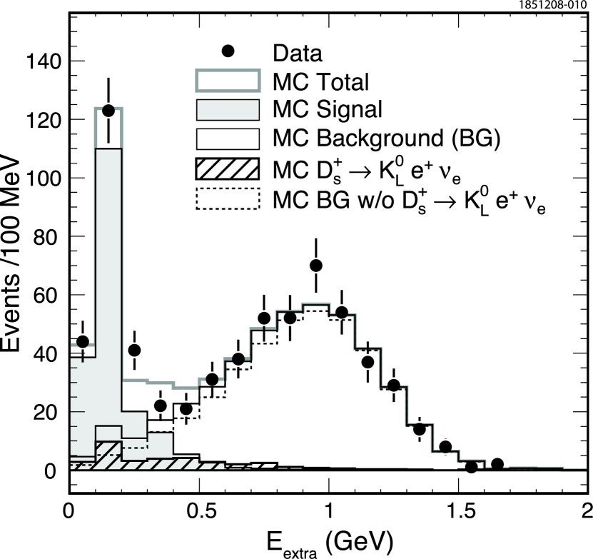
Figure 2: Distribution of $E_{\text{extra}}$ after $\Delta M(D_{s})$ sideband subtraction. Filled circles are from data and histograms are obtained from MC simulation. The MC signal and peaking background ($D^{+}_{s}\rightarrow K^{0}_{L}e^{+}\nu_{e}$) components are normalized to our measured branching fractions. The errors shown are statistical only.

III.3 Background estimation

After the $\Delta M(D_{s})$ sideband subtraction, two significant components of background remain. One is from $D^{+}_{s}\rightarrow K^{0}_{L}e^{+}\nu_{e}$ decay. If the $K^{0}_{L}$ deposits little or no energy in the calorimeter, this decay mode has an $E_{\text{extra}}$ distribution very similar to the signal, peaking well below $400$ MeV. The second source, other $D_{s}$ semielectronic decays, rises smoothly with increasing $E_{\text{extra}}$, up to $1$ GeV. Estimates of these backgrounds are also shown in Fig. 2. The optimal signal region in $E_{\text{extra}}$ for DT yield extraction is predicted from an MC simulation study. Choosing $E_{\text{extra}}$ less than $400$ MeV maximizes the signal significance. Note that with our chosen requirement of $E_{\text{extra}}<400$ MeV, we are including $D^{+}_{s}\to\tau^{+}\nu_{\tau}\gamma$ as signal. However, this is expected to be very small, as the kinetic energy of the $\tau^{+}$ in the $D^{+}_{s}$ rest frame is only $9.3$ MeV and it cannot radiate much.

The number of nonpeaking background events $b_{\text{np}}$ in the $E_{\text{extra}}$ signal region is estimated from the number of events in the $E_{\text{extra}}$ sideband region between $0.6$ GeV and $2$ GeV, scaled by the MC-determined ratio $c_{b}$ ($\equiv b^{\text{(l)}}/b^{\text{(h)}}$) of the number of background events in the $E_{\text{extra}}$ signal region, $b^{\text{(l)}}$, to the number of events in the $E_{\text{extra}}$ sideband region, $b^{\text{(h)}}$. The number of peaking background events $b_{\text{p}}$ due to the $D^{+}_{s}\rightarrow K^{0}_{L}e^{+}\nu_{e}$ decay is determined by using the expected number from MC simulation. The overall expected number of background events in the $E_{\text{extra}}$ signal region, $b$, is computed as follows:

$$b=b_{\text{np}}+b_{\text{p}}=c_{b}b^{\text{(h)}}(\text{data})+b(K^{0}_{L}e^{+}\nu_{e})_{\text{MC}},$$ (7)

where $b^{\text{(h)}}(\text{data})$ is the number of data events in the $E_{\text{extra}}$ sideband region and $b(K^{0}_{L}e^{+}\nu_{e})_{\text{MC}}$ is the number of background events due to $D^{+}_{s}\rightarrow K^{0}_{L}e^{+}\nu_{e}$ as estimated from our MC simulation. We normalize this quantity using our measured koloina $\mathcal{B}(D^{+}_{s}\rightarrow K^{0}_{S}e^{+}\nu_{e})=(0.19\pm 0.05\pm 0.01)\%$. We simulate calorimeter response to $K^{0}_{L}$ using a momentum dependent $K^{0}_{L}$ interaction probability density function obtained from studying $\psi(3770)\to D^{0}\bar{D}^{0}$ events in which the $\bar{D}^{0}$ has been reconstructed in hadronic tag modes and the $D^{0}$ decays to the $K^{0}_{L}\pi^{+}\pi^{-}$ final state.

The numbers of estimated background events from peaking and nonpeaking sources in each tag mode are summarized in Table 2.

Table 2: Estimated backgrounds in the extra energy signal region below $400$ MeV in each tag mode. Here $b_{\text{p}}$ is the peaking background from $D^{+}_{s}\to K^{0}_{L}e^{+}\nu_{e}$ decay, $b_{\text{np}}$ is the nonpeaking background from other $D_{s}$ semileptonic decays, and $b$ is the total number of background events. The errors shown are statistical only.

Tag mode	$b_{\text{np}}$	$b_{\text{p}}$	$b$
$D_{s}^{-}\rightarrow\phi\pi^{-}$	$11.8\pm 1.0$	$7.7\pm 0.5$	$19.4\pm 1.1$
$D_{s}^{-}\rightarrow K^{-}K^{\ast 0}$	$12.2\pm 1.1$	$8.7\pm 0.5$	$20.9\pm 1.3$
$D_{s}^{-}\rightarrow K^{-}K^{0}_{S}$	$4.6\pm 0.7$	$4.5\pm 0.3$	$9.1\pm 0.7$
Total	$28.5\pm 1.7$	$20.9\pm 0.8$	$49.4\pm 1.8$

IV Results

The signal efficiency determined by MC simulation has been weighted by the ST yields in each mode as shown in Table 3. We determine the weighted average signal efficiency $\epsilon=(72.4\pm 0.3)\%$ for the decay chain $D^{+}_{s}\to\tau^{+}\nu_{\tau}\to e^{+}\nu_{e}\bar{\nu}_{\tau}\nu_{\tau}$.

Table 3: Summary of the signal efficiency determined by MC simulation. Average efficiency $\epsilon$ and the tag bias $b_{\text{tag}}$ are obtained by using the weighting factor $w$ determined from single-tag yields in data.

Tag mode	$w$	$\epsilon\equiv\epsilon_{\text{DT}}/\epsilon_{\text{ST}}$	$b_{\text{tag}}=\epsilon^{\prime}_{\text{ST}}/\epsilon_{\text{ST}}$
$D_{s}^{-}\rightarrow\phi\pi^{-}$	$0.3671$	$0.6964\pm 0.0046$	$1.0089\pm 0.0058$
$D_{s}^{-}\rightarrow K^{-}K^{\ast 0}$	$0.4154$	$0.7337\pm 0.0049$	$1.0061\pm 0.0060$
$D_{s}^{-}\rightarrow K^{-}K^{0}_{S}$	$0.2175$	$0.7536\pm 0.0054$	$1.0032\pm 0.0065$
Average		$0.7244\pm 0.0029$	$1.0065\pm 0.0036$

The DT yields with the $400$ MeV extra energy requirement are summarized in Table 4. We find $n_{\text{DT}}=180.6\pm 15.9$ summed over all tag modes. Using $\mathcal{B}(\tau^{+}\rightarrow e^{+}\nu_{e}\bar{\nu}_{\tau})=(17.85\pm 0.05)\%$ Amsler:2008zz , we obtain the leptonic decay branching fraction $\mathcal{B}(D^{+}_{s}\rightarrow\tau^{+}\nu_{\tau})=(5.30\pm 0.47)\%$, where the uncertainty is statistical.

Table 4: Summary of double-tag (DT) yields in each tag mode, where $n^{\text{S}}_{\text{DT}}$ is the DT yield in the tag mass signal region, $n^{\text{B}}_{\text{DT}}$ is the yield in the tag mass sideband region, $s$ is the tag mass sideband scaling factor, $b$ is the number of estimated background in the extra energy signal region after tag mass sideband scaled background subtraction, and $n_{\text{DT}}$ is the background subtracted DT yield. The errors shown are statistical only.

Tag mode	$n^{\text{S}}_{\text{DT}}$	$n^{\text{B}}_{\text{DT}}$	$s$	$b$	$n_{\text{DT}}$
$D_{s}^{-}\rightarrow\phi\pi^{-}$	$79$	$1$	$0.980$	$19.4\pm 1.1$	$58.6\pm 9.0$
$D_{s}^{-}\rightarrow K^{-}K^{\ast 0}$	$110$	$6$	$1.000$	$20.9\pm 1.3$	$83.1\pm 10.8$
$D_{s}^{-}\rightarrow K^{-}K^{0}_{S}$	$50$	$2$	$0.999$	$9.1\pm 0.7$	$38.9\pm 7.2$
Total				$49.4\pm 1.8$	$180.6\pm 15.9$

V Systematic Uncertainty

Sources of systematic uncertainties and their effects on the $D^{+}_{s}\to\tau^{+}\nu_{\tau}$ branching fraction determination are summarized in Table 5.

Table 5: Summary of sources of systematic uncertainty and their effects on the branching fraction measurement.

Source	Effect on $\mathcal{B}$ $(\%)$
Background (nonpeaking)	$0.7$
$D^{+}_{s}\to K^{0}_{L}e^{+}\nu_{e}$ (peaking)	$3.2$
Extra shower	$1.1$
Extra track	$1.1$
$Q_{\text{net}}=0$	$1.1$
Non electron	$0.1$
Secondary electron	$0.3$
Number of tag	$0.4$
Tag bias	$0.2$
Tracking	$0.3$
Electron identification	$1.0$
FSR	$1.0$
Total	$4.1$

We considered six semileptonic decays, $D^{+}_{s}\to$ $\phi e^{+}\nu_{e}$, $\eta e^{+}\nu_{e}$, $\eta^{\prime}e^{+}\nu_{e}$, $K^{0}e^{+}\nu_{e}$, $K^{\ast 0}e^{+}\nu_{e}$, and $f_{0}e^{+}\nu_{e}$, as the major sources of background in the $E_{\text{extra}}$ signal region. The second dominates the nonpeaking background, and the fourth (with $K^{0}_{L}$) dominates the peaking background. Uncertainty in the signal yield due to nonpeaking background ($0.7\%$) is assessed by varying the semileptonic decay branching fractions by the precision with which they are known koloina . Imperfect knowledge of $\mathcal{B}(D^{+}_{s}\to K^{0}e^{+}\nu_{e})$ gives rise to a systematic uncertainty in our estimate of the amount of peaking background in the signal region, which has an effect on our branching fraction measurement of $3.2\%$.

We study differences in efficiency, data vs MC events, due to the extra energy requirement, extra track veto, and $Q_{\text{net}}=0$ requirement, by using samples from data and MC events, in which both the $D_{s}^{-}$ and $D_{s}^{+}$ satisfy our tag requirements, i.e., “double-tag” events. We then apply each of the above-mentioned requirements and compare loss in efficiency of data vs MC events. In this way we obtain a correction of $1.6\%$ for the extra energy requirement and systematic uncertainties on each of the three requirements of $1.1\%$ (all equal, by chance).

The non-$e^{+}$ background in the signal $e^{+}$ candidate sample is negligible ($0.4\%$) due to the low probability ($\sim 0.1\%$ per track) that hadrons ($\pi^{+}$ or $K^{+}$) are misidentified as $e^{+}$ Adam:2006nu . Uncertainty in these backgrounds produces a $0.1\%$ uncertainty in the measurement of $\mathcal{B}(D^{+}_{s}\rightarrow\tau^{+}\nu_{\tau})$. The secondary $e^{+}$ backgrounds from charge symmetric processes, such as $\pi^{0}$ Dalitz decay ($\pi^{0}\to e^{+}e^{-}\gamma$) and $\gamma$ conversion ($\gamma\to e^{+}e^{-}$), are assessed by measuring the wrong-sign signal electron in events with $Q_{\text{net}}=\pm 2$. The uncertainty in the measurement from this source is estimated to be $0.3\%$.

Other possible sources of systematic uncertainty include $n_{\text{ST}}$ ($0.4\%$), tag bias ($0.2\%$), tracking efficiency ($0.3\%$), $e^{\pm}$ identification efficiency ($1\%$), and FSR ($1\%$). Combining all contributions in quadrature, the total systematic uncertainty in the branching fraction measurement is estimated to be $4.1\%$.

VI Summary

In summary, using the sample of $26\,334$ tagged $D^{+}_{s}$ decays with the CLEO-c detector we obtain the absolute branching fraction of the leptonic decay $D^{+}_{s}\rightarrow\tau^{+}\nu_{\tau}$ through $\tau^{+}\rightarrow e^{+}\nu_{e}\bar{\nu}_{\tau}$

$$\mathcal{B}(D^{+}_{s}\rightarrow\tau^{+}\nu_{\tau})=(5.30\pm 0.47\pm 0.22)\%,$$ (8)

where the first uncertainty is statistical and the second is systematic. This result supersedes our previous measurement :2007zm of the same branching fraction, which used a subsample of data used in this work.

The decay constant $f_{D_{s}}$ can be computed using Eq. (1) with known values Amsler:2008zz $G_{F}=1.16637(1)\times 10^{-5}$ GeV^-2, $m_{D_{s}}=1968.49(34)$ MeV, $m_{\tau}=1776.84(17)$ MeV, and $\tau_{D_{s}}=500(7)\times 10^{-15}$ s. We assume $|V_{cs}|=|V_{ud}|$ and use the value $0.97418(26)$ given in Ref. Towner:2007np . We obtain

$$f_{D_{s}}=(252.5\pm 11.1\pm 5.2)\text{MeV}.$$ (9)

Combining with our other determination Syracuse:2008new of $f_{D_{s}}=(263.3\pm 8.2\pm 3.9)$ MeV with $D^{+}_{s}\to\mu^{+}\nu_{\mu}$ and $D^{+}_{s}\to\tau^{+}\nu_{\tau}$ ($\tau^{+}\to\pi^{+}\bar{\nu_{\tau}}$) decays, we obtain

$$f_{D_{s}}=(259.5\pm 6.6\pm 3.1)\text{MeV}.$$ (10)

This result is derived from absolute branching fractions only and is the most precise determination of the $D_{s}$ leptonic decay constant to date.

Our combined result is larger than the recent LQCD calculation $f_{D_{s}}=(241\pm 3)$ MeV Follana:2007uv by $2.3$ standard deviations. The difference between data and LQCD for $f_{D_{s}}$ could be due to physics beyond the SM Dobrescu:2008er , unlikely statistical fluctuations in the experimental measurements or the LQCD calculation, or systematic uncertainties that are not understood in the LQCD calculation or the experimental measurements.

Combining with our other determination Syracuse:2008new of $\mathcal{B}(D^{+}_{s}\rightarrow\tau^{+}\nu_{\tau})=(6.42\pm 0.81\pm 0.18)\%$, via $\tau^{+}\to\pi^{+}\bar{\nu}_{\tau}$, we obtain

$$\mathcal{B}(D^{+}_{s}\rightarrow\tau^{+}\nu_{\tau})=(5.62\pm 0.41\pm 0.16)\%.$$ (11)

Using this with our measurement Syracuse:2008new of $\mathcal{B}(D^{+}_{s}\rightarrow\mu^{+}\nu_{\mu})=(0.565\pm 0.045\pm 0.017)\%$, we obtain the branching fraction ratio

$$R=\frac{\mathcal{B}(D^{+}_{s}\rightarrow\tau^{+}\nu_{\tau})}{\mathcal{B}(D^{+}_{s}\to\mu^{+}\nu_{\mu})}=10.1\pm 0.9\pm 0.3.$$ (12)

This is consistent with $9.76$, the value predicted by the SM with lepton universality, as given in Eq. (1) with known masses Amsler:2008zz .

References

(1)
N. Cabibbo,
Phys. Rev. Lett. 10, 531 (1963).
(2)
M. Kobayashi and T. Maskawa,
Prog. Theor. Phys. 49, 652 (1973).
(3)
C. Amsler et al. (Particle Data Group),
Phys. Lett. B 667, 1 (2008).
(4)
K. Ikado et al. (Belle Collaboration),
Phys. Rev. Lett. 97, 251802 (2006).
(5)
B. Aubert et al. (BABAR Collaboration),
Phys. Rev. D 77, 011107 (2008).
(6)
A. G. Akeroyd and C. H. Chen,
Phys. Rev. D 75, 075004 (2007);
A. G. Akeroyd,
Prog. Theor. Phys. 111, 295 (2004).
(7)
J. L. Hewett,
arXiv:hep-ph/9505246.
(8)
W. S. Hou,
Phys. Rev. D 48, 2342 (1993).
(9)
E. Follana, C. T. H. Davies, G. P. Lepage, and J. Shigemitsu
(HPQCD Collaboration),
Phys. Rev. Lett. 100, 062002 (2008).
(10)
B. I. Eisenstein et al. (CLEO Collaboration),
Phys. Rev. D 78, 052003 (2008).
(11)
B. A. Dobrescu and A. S. Kronfeld,
Phys. Rev. Lett. 100, 241802 (2008).
(12)
D. Cronin-Hennessy et al. (CLEO Collaboration),
arXiv:0801.3418.
(13)
M. Artuso et al. (CLEO Collaboration),
Phys. Rev. Lett. 99, 071802 (2007).
(14)
K. M. Ecklund et al. (CLEO Collaboration),
Phys. Rev. Lett. 100, 161801 (2008).
(15)
J. P. Alexander et al. (CLEO Collaboration),
Phys. Rev. D 79, 052001 (2009).
(16)
R. A. Briere et al. (CESR-c and CLEO-c Taskforces, CLEO-c Collaboration),
Cornell University, LEPP Report No. CLNS 01/1742 (2001) (unpublished).
(17)
Y. Kubota et al. (CLEO Collaboration),
Nucl. Instrum. Meth. A 320, 66 (1992).
(18)
D. Peterson et al., Nucl. Instrum. Methods Phys. Res., Sec. A
478, 142 (2002).
(19)
M. Artuso et al., Nucl. Instrum. Methods Phys. Res., Sec. A 502, 91 (2003).
(20)
R. Brun et al., GEANT 3.21, CERN Program Library
Long Writeup W5013 (unpublished) 1993.
(21) D. J. Lange, Nucl. Instrum. Methods Phys. Res., Sec. A
462, 152 (2001).
(22)
S. Dobbs et al. (CLEO Collaboration),
Phys. Rev. D 76, 112001 (2007).
(23)
J. P. Alexander et al. (CLEO Collaboration),
Phys. Rev. Lett. 100, 161804 (2008).
(24)
E. Barberio and Z. Wa̧s, Comput. Phys. Commun. 79, 291 (1994).
(25)
J. Yelton et al. (CLEO Collaboration),
arXiv:0903.0601.
(26)
N. E. Adam et al. (CLEO Collaboration),
Phys. Rev. Lett. 97, 251801 (2006).
(27)
I. S. Towner and J. C. Hardy,
Phys. Rev. C 77, 025501 (2008).