Abstract

A novel formalism for Bayesian learning in the context of complex inference models is proposed. The method is based on the use of the Stationary Fokker–Planck (SFP) approach to sample from the posterior density. Stationary Fokker–Planck sampling generalizes the Gibbs sampler algorithm for arbitrary and unknown conditional densities. By the SFP procedure approximate analytical expressions for the conditionals and marginals of the posterior can be constructed. At each stage of SFP, the approximate conditionals are used to define a Gibbs sampling process, which is convergent to the full joint posterior. By the analytical marginals efficient learning methods in the context of Artificial Neural Networks are outlined. Off–line and incremental Bayesian inference and Maximum Likelihood Estimation from the posterior is performed in classification and regression examples. A comparison of SFP with other Monte Carlo strategies in the general problem of sampling from arbitrary densities is also presented. It is shown that SFP is able to jump large low–probabilty regions without the need of a careful tuning of any step size parameter. In fact, the SFP method requires only a small set of meaningful parameters which can be selected following clear, problem–independent guidelines. The computation cost of SFP, measured in terms of loss function evaluations, grows linearly with the given model’s dimension.

1 Introduction

Parameter inference from limited and noisy data in complex nonlinear models is a common and necessary step among many disciplines in modern science and engineering. A prominent framework to extract nonlinear relations from data is given by Artificial Neural Networks (ANN’s). These formal constructs are flexible enough to learn extremely complicated maps. However, the potential power of ANN’s is usually limited in practice because the network size must be bounded in order to avoid poor generalization (i.e. out of sample) performance. Authors like [Neal, 1996] and [MacKay, 1992] have given strong arguments that favor a Bayesian perspective, in which the so called overtraining problem is alleviated. This Bayesian approach has proven its effectiveness in a number of applications [Auld, 2007, Chib et al., 2002, Jalobeanu et al., 2002]. However, Bayesian inference based on the use of the full posterior density (i.e. not limited to a small subset of the posterior modes) usually demands very intensive computation [Neal, 1996]. Several techniques oriented to improve efficiency have been proposed. Variational Bayes [Ghahramani & Beal., 2001, Nakajima & Watanabe, 2007], a method that has been mainly applied to particular inference procedures like hidden Markov models and graphical models, is a promising tool where the posterior is approximated by simple distributions. Approaches based on genetic programming also seem valuable [Marwala, 2007], but their usefulness has not yet been established for large scale systems. Here is introduced a new paradigm from which a proper Bayesian estimation for large complex models can be done in the basis of a Gibbs sampling for the given model’s weights. This makes the procedure of relatively low computation cost and this cost increases slowly as the inference model’s dimension grows. Moreover, from the proposed method approximate closed expressions for the posterior marginals can be derived. As far as the author of the present Letter knows, this is the first approach that admits the construction of analytic expressions for the posterior density marginals. This is useful in a number of ways. It permits the definition of efficient maximum likelihood and incremental learning methods. Maximum likelihood can be used to drastically reduce the computation cost for the trained inference models, making them suitable for chip implementation, for instance. Incremental learning on the other hand, gives a way to manage data that dynamically arrives to the inference system, enlarging the horizons for the applications of Bayesian techniques.

The proposed method admits an arbitrary close approximation to the posterior, with a computational effort that is controlled through a small set of meaningful parameters. Also, the formalism is directly connected with equilibrium statistical mechanics. The approach is general, but in this contribution it’s validity is tested on three layered ANN’s of increasing size. A classification benchmark problem and two regression problems consisting of real time series with well documented difficulty and experimental interest are considered. A discussion of the approach in the larger context of Monte Carlo methods for sampling is also presented.

The proposed method is based on a recently introduced algorithm for density estimation in stochastic search processes, namely the Stationary Fokker–Planck sampling (SFP) strategy [Berrones, 2008]. This algorithm learns the stationary density of a general stochastic search in a potential with high dimension $V(x_{1},x_{2},...,x_{n},...,x_{N})$, using only one–dimensional linear operators. Essentialy, SFP consists on projecting the multi–dimensional Fokker–Planck equation associated to the stochastic search into a one–dimensional equation for the stationary conditional cumulative distributions, $y(x_{n}|\{x_{j\neq n}=x_{j}^{*}\})=\int_{-\infty}^{x_{n}}p(x^{{}^{\prime}}_{n}|\{x_{j\neq n}=x_{j}^{*}\})dx^{{}^{\prime}}_{n}$. The starting point is the following stochastic search defined over $L_{1,n}\leq x_{n}\leq L_{2,n}$,

$$\dot{x}_{n}=-\frac{\partial V}{\partial x_{n}}+\varepsilon(t),$$ (1)

where $\varepsilon(t)$ is an additive noise with zero mean. The model given by Eq.(1) can be interpreted as an overdamped nonlinear dynamical system composed by $N$ interacting particles. The temporal evolution of the probability density of such a system in the presence of an additive Gaussian white noise, is described by a linear differential equation, the Fokker – Planck equation [Risken, 1984, Van Kampen, 1992],

$$\dot{p}(x)=\sum_{n=1}^{N}\frac{\partial}{\partial x_{n}}\Big{[}\frac{\partial V}{\partial x_{n}}p(x)\Big{]}+D\sum_{n=1}^{N}\sum_{m=1}^{N}\frac{\partial^{2}p(x)}{\partial x_{n}\partial x_{m}},$$ (2)

where $D$ is a constant, called diffusion constant, that is proportional to the noise strength. The direct use of Eq. (2) for optimization or deviate generation purposes would imply the calculation of high dimensional integrals. It results numerically much less demanding to perform the following one dimensional projection of Eq. (2). Under very general conditions (e. g., the absence of infinite cost values), the equation (2) has a stationary solution over a search space with reflecting boundaries [Risken, 1984, Grasman & van Herwaarden, 1999]. The stationary conditional probability density satisfy the one dimensional Fokker – Planck equation

$$D\frac{\partial p(x_{n}|\{x_{j\neq n}=x_{j}^{*}\})}{\partial x_{n}}+p(x_{n}|\{x_{j\neq n}=x_{j}^{*}\})\frac{\partial V}{\partial x_{n}}=0.$$ (3)

From Eq. (3) follows a linear second order differential equation for the cumulative distribution $y(x_{n}|\{x_{j\neq n}=x_{j}^{*}\})=\int_{-\infty}^{x_{n}}p(x^{{}^{\prime}}_{n}|\{x_{j\neq n}=x_{j}^{*}\})dx^{{}^{\prime}}_{n}$,

$$\frac{d^{2}y}{dx_{n}^{2}}+\frac{1}{D}\frac{\partial V}{\partial x_{n}}\frac{dy}{dx_{n}}=0,$$ (4)

$$y(L_{1,n})=0,\quad y(L_{2,n})=1.$$

Random deviates can be drawn from the density $p(x_{n}|\{x_{j\neq n}=x_{j}^{*}\})$ by the fact that $y$ is a uniformly distributed random variable in the interval $y\in[0,1]$. Viewed as a function of the random variable $x_{n}$, $y(x_{n}|\{x_{j\neq n}\})$ can be approximated through a linear combination of functions from a complete set that satisfy the boundary conditions in the interval of interest,

$$\hat{y}(x_{n}|\{x_{j\neq n}\})=\sum_{l=1}^{L}a_{l}\varphi_{l}(x_{n}).$$ (5)

Choosing for instance, a basis in which $\varphi_{l}(0)=0$, the $L$ coefficients are uniquely defined by the evaluation of Eq. (4) in $L-1$ interior points. In this way, the approximation of $y$ is performed by solving a set of $L$ linear algebraic equations, involving $L-1$ evaluations of the derivative of $V$.

The SFP sampling is based on the iteration of the following steps:

1) Fix the variables $x_{j\neq n}=x_{j}^{*}$ and approximate $y(x_{n}|\{x_{j\neq n}\})$ by the use of formulas (4) and (5).

2) By the use of $\hat{y}(x_{n}|\{x_{j\neq n}\})$ construct a lookup table in order to generate a deviate $x_{n}^{*}$ drawn from the stationary distribution $p(x_{n}|\{x_{j\neq n}=x_{j}^{*}\})$.

3) Update $x_{n}=x_{n}^{*}$ and repeat the procedure for a new variable $x_{j\neq n}$.

The fundamental parameters of SFP sampling, $L$ and $D$, have a clear meaning, which is very helpful for their selection. The diffusion constant “smooth” the density. This is evident by taking the limit $D\to\infty$ in Eq. (4), which imply a uniform density in the domain. The number of base functions $L$, on the other hand, defines the algorithm’s capability to “learn” more or less complicated density structures. Therefore, for a given $D$, the number $L$ should be at least large enough to assure that the estimation algorithm will generate valid distributions $y(x_{n}|\{x_{j\neq n}\})$. A valid distribution should be a monotone increasing continuos function that satisfy the boundary conditions. The parameter $L$ ultimately determines the computational cost of the procedure, because at each iteration a system of size $\propto L$ of linear algebraic equations must be solved $N$ times. Therefore, the user is able to control the computational cost through the interplay of the two basic parameters: for a larger $D$ a smoother density should be estimated, so a lesser $L$ can be used.

It should be noticed that SFP is a generalization of Gibbs sampling. Therefore, the deviates generated by the iterative procedure are in the long run sampled from the full joint equilibrium density

$$p(x_{1},x_{2},...,x_{n},...,x_{N})=\left(\frac{1}{Z}\right)\exp(-V/D),$$ (6)

where $Z$ is a normalization factor. Additionaly, a convergent representation for $y(x_{n})$ is obtained after taking the average of the coefficients $a$’s in the expansion (5) over the iterations [Berrones, 2008],

$$\left<\hat{y}\right>=\sum_{l=1}^{L}\left<a_{l}\right>\varphi_{l}(x_{n})\to y(x_{n}),$$ (7)

Under general conditions, the Gibbs sampler converges at a geometric rate [Roberts & Polson, 1994, Canty, 1999] and there is some evidence that this fast convergence is shared by SFP [Berrones, 2009]. In the next section the properties of the SFP sampler are studied in the wider context of Monte Carlo methods. Thereafter the general toolkit for Bayesian inference based on SFP is developed and tested.

2 SFP sampler

In order to sample a given distribution $\pi(\vec{x})$, the potential function that enters into SFP should be given by

$$V(\vec{x})=-\ln\pi(\vec{x}),$$ (8)

using $D=1$. The correct normalization is directly obtained by construction without explicitly calculating it nor including it in the definition of $V$. The advantages of SFP sampling with respect to previous Monte Carlo methods are first illustrated through an important class of probability densities, namely the separable probability densities of the form

$$\pi(\vec{x})=\prod_{i=1}^{N}f(x_{i}).$$ (9)

In this case SFP converges in a single iteration. This result follows from the fact that the dynamics (1) associated to the random search decouples into $N$ independent one dimensional stochastic differential equations, which makes the Gibbs sampling stage (steps 2 and 3) of SFP unnecessary. Because $D$ is fixed, SFP requiers a single parameter, $L$. But $L$ simply refers to the number of base functions used in expansion (5), so in SFP there is no need to adjust a step size parameter. Step size parameters are difficult to tune because their correct selection depends on the actual variance of the sampled distribution, which in general is unknown. The parameter $L$ on the other hand, is selected by objective criteria that are independent from any knowledge about the sampled density. Specifically, $L$ should be large enough such that the observed marginals are valid probability densities. Consider the next example, a one dimensional mixture density given by

$$q(x)=\sum_{i=1}^{R}r_{i}f_{i}(x),$$ (10)

where $f_{i}(x)$ are normal densities $N(\mu_{i},\sigma_{i})$. It has been pointed out in the literature that mixture densities with well separated modes are difficult to sample by Monte Carlo methods [Celeux et al., 2000, Marin et al., 2005]. Consider a case with three modes, which result from the mixture of normal densities $\pi(x)=0.2N(5,2)+0.2N(20,2)+0.6N(40,2)$. This mixture density has mean and standard deviation $\mu=29$ and $\sigma=14.35$ respectively. The Figure 1 shows the resulting estimation of the density after a single SFP iteration with $L=1100$.

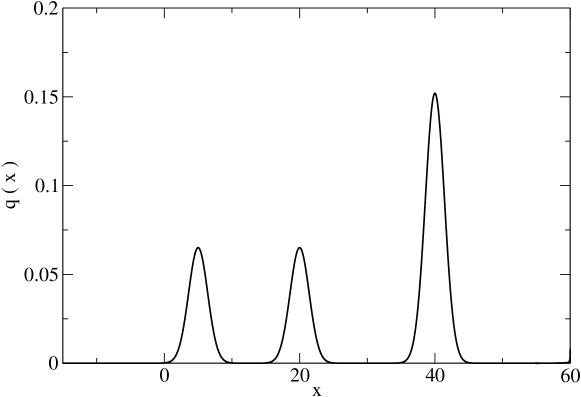
Figure 1: Density estimated by SFP for the mixture density problem.

In all the numerical experiments discussed in this Letter, a Fourier basis is used in formula (5) to approximate the distributions produced by SFP sampling,

$$\hat{y}=\sum_{l=1}^{L}a_{l}\sin\left((2l-1)\frac{\pi(x_{n}-L_{1,n})}{2(L_{2,n}-L_{1,n})}\right).$$ (11)

In the estimation of the mixture density, the parameter $L$ has been chosen by growing it’s size by $200$ units per experiment, starting at $L=100$. After each experiment the resulting density is visually inspected and it’s variance is calculated by direct integration from the formula Eq. (5). It’s selected the minimum value of $L$ which produce a valid density with positive variance. Each SFP iteration takes around $4$ seconds in the equipment used (details of which are given in Section 4). Points from this density are easly drawn by the construction of a lookup table for the cumulative distribution Eq. (5) to generate each deviate as in step 2 of SFP. Figure 2 shows a sample of $500$ points whose generation took a fraction of a second. The auto–correlation function for the sample is also plotted. No significant correlations appear between the points in the sample. The average and standard deviation estimated from the sample are $\hat{\mu}=27.31$ and $\hat{\sigma}=14.6$ respectively.

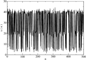
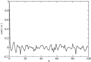
Figure 2: Sample generated by SFP and it’s autocorrelation function for the mixture density problem.

The same mixture density sampling problem is studied by the Metropolis and Hybrid Markov–Chain Montecarlo (HMCMC) algorithms. The implementations provided in the “Software for flexible Bayesian modeling and Markov chain sampling” developed by Radford Neal (downloadable at http://www.cs.toronto.edu/$\sim$radford/) are used. The parameters for the Metropolis and HMCMC have been carefully tuned in order to have acceptable rejections rates, which are $0.7$ for Metropolis and $0.78$ for HMCMC. Samples of $1000$ points provided by both methods are presented in Fig. 3. The estimated average from both samples is around the value of $5$.

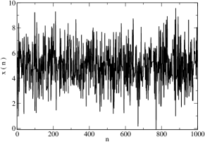
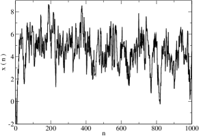
Figure 3: Samples generated by Metropolis (first graph) and HMCMC (second graph) for the mixture density problem. Both samplings remain trapped in a local region of the relevant search space.

These results show one of the main drawbacks in many Monte Carlo strategies, namely the possibility to reach a state of apparent equilibrium which in fact is unrepresentative of the whole density. The mixture density example illustrates what might be one of the most promising features of SFP: it’s capacity to jump large regions of low probability, reducing the danger of getting trapped into local high probability regions.

For multidimensional non–separable distributions the Gibbs sampling stage of SFP is essential. Consider the following example, provided in the tutorial of the “Software for flexible Bayesian modeling and Markov chain sampling”,

$$V(\vec{x})=\frac{1}{2}(x^{2}+y^{2}+z^{2})+(x+y+z)^{2}+10000/(1+x^{2}+y^{2}+z^{2}),$$ (12)

which gives a three–dimensional ring density. The Table 1 lists the results of the estimated expectations for each one of the variables from $2000$ points generated by the samplers without rejecting initial points. By symmetry, the correct expected values are equal to zero. For SFP $L=150$ in the search space defined by the cube $[-20,20]^{3}$. The parameters for HMCMC and Metropolis are the same as discussed in the software’s tutorial.

	E(x)	E(y)	E(z)
SFP	-0.04	-0.5	0.54
HMCMC	0.48	-0.18	-0.31
Metropolis	1.92	-0.61	-1.35

Table 1: Estimations of the mean values by SFP, HMCMC and Metropolis algorithms in the three–dimensional ring distribution problem. By the symmetries of the sampled distribution, the true mean values are equal to zero for all the three variables. SFP and HMCMC display similar results.

The SFP and HMCMC methods display similar estimations of the expected values while the Metropolis algorithm shows a significantly poorer performance. The power spectrum of the samples generated by the different methods has been studied. It has turned out that SFP has a power spectrum which is consistent with a random walk, a behavior shared with Metropolis and with many other Monte–Carlo approaches. The HMCMC method on the other hand, shows a power spectrum which indicates exponential decay in the autocorrelations. However, perfectly independent samples of the marginals (which might be of interest in several applications) can be generated by the use of SFP. The estimated analytic forms of the marginal densities of the ring distribution are shown in Fig. 4. Figure 5 is a plot of the sample generated by SFP in the $x-y$ plane, which indicates that SFP captures the interactions among variables.

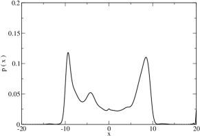
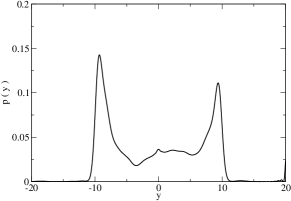
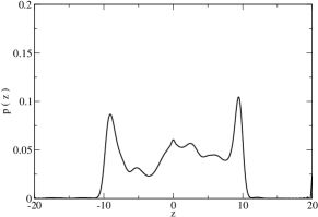
Figure 4: Marginals estimated by SFP for the three–dimensional ring problem.

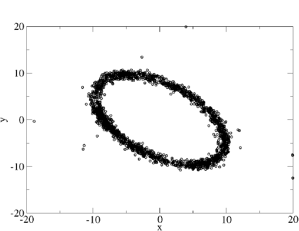
Figure 5: Plot in the $x-y$ plane of a sample generated by SFP of the three–dimensional ring problem.

An additional comparison of SFP with the family of Monte Carlo strategies based on Langevin diffusions is given in the ground of the sampling of mixture densities in several dimensions. As already pointed out, this is a difficult task for many samplers, specially when the mixture has well separated modes. In [Roberts & Stramer, 2002] is proposed a mixture of two bivariate Gaussians in order to test the performance of different Langevin-diffusion based algorithms. The mixture is the following, $\pi(\vec{x})=0.5N(\vec{\mu}_{1},\Sigma)+0.5N(\vec{\mu}_{2},\Sigma)$ with $\vec{\mu}_{1}=(6,-5)^{T}$, $\vec{\mu}_{2}=(-2,3)^{T}$ and $\Sigma=\bar{I}$. The Figure 6 shows the generation of $15000$ sample points by SFP with $L=200$ in a search space $[-10,10]^{2}$. This graph can be directly compared with the experiments reported in [Roberts & Stramer, 2002]. It is clear that SFP is able to very quickly find the two modes of the mixture. The rapid switching between modes seems to outperform Langevin diffusions.

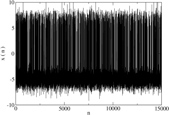
Figure 6: Sample generated by SFP for a mixture of two bivariate Gaussians.

In the Figure 7 the sample generated by SFP in the $x-y$ plane is plotted. The straight lines show that there is a positive probability that during the SFP iterations a conditional $p(x|y)$ that detect both modes is drawn. This is how SFP eventually mix over the two modes. In this sense, SFP connects the search space through the $x$ direction given that there is some overlap of the modes in the $y$ direction. Some deviates lie on the border of the search space. This effect is a consequence of the discretization used to solve the stationary Fokker-Planck equation. With a larger $L$, the marginals are approximated more closely and the border effect can be corrected, at the cost of a larger computation effort.

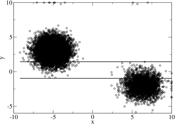
Figure 7: Plot in the $x-y$ plane of a sample generated by SFP for a mixture of two bivariate Gaussians. The straight lines show that there is a positive probability that during the iterations of a given SFP run a conditional $p(x|y)$ that detect both modes will be drawn.

A very difficult task occurs when a mixture effectively split a large search space into several distant unconnected regions. The following case is considered, $\pi(\vec{x})=0.2N(\vec{\mu}_{1},\Sigma)+0.2N(\vec{\mu}_{2},\Sigma)+0.6N(\vec{\mu}_{3},\Sigma)$ with $\vec{\mu}_{1}=(5,0)^{T}$, $\vec{\mu}_{2}=(20,10)^{T}$, $\vec{\mu}_{3}=(40,20)^{T}$ and

$$\Sigma=\left(\begin{array}[]{ccc}2&0.5\\ 0.5&2\\ \end{array}\right)$$ (15)

For this example SFP is unable to find the three modes in a reasonable amount of time. It is however possible to easily sample this density if values $D>1$ are allowed. By exploring with diffusion coefficients slightly larger than $D=1$ the user is able to consider approximated densities with extra noise in which the search space is connected. In the Figure 8 a $500$ points sample with $L=300$ and $D=1.1$ in the search space $[0,60]^{2}$ is plotted, showing that SFP is capable to detect all of the modes, with the sample points distributed among them in consistency with the underlying mixture.

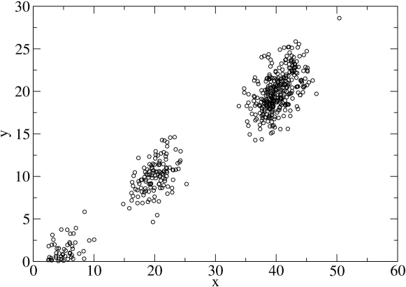
Figure 8: Plot in the $x-y$ plane of a sample generated by SFP for a mixture of three bivariate Gaussians.

A more careful comparison of SFP with several Monte Carlo methods for sampling is a topic which deserves further research. From the results given so far it is however possible to establish a list of general statements about how SFP relates with other Monte Carlo procedures:

• SFP generalizes the Gibbs sampler for cases in which the conditionals are not explicitly known. Therefore SFP inherits many of the advantages and drawbacks of the Gibbs sampler.

• There is no need for a step size parameter, which is one of the main computational advantages of the Gibbs sampler and SFP.

• Like for the Gibbs sampler, the samples generated by SFP display a random walk behavior. In this regard, the Monte Carlo methods which include momentum appear to be superior than SFP when almost independent samples are required. However, perfectly independent samples for the marginals can be generated by SFP (a property not shared by the Gibbs sampler).

• Like the Monte Carlo methods based on Langevin diffusions, SFP requires the numerical evaluation of the gradient of the sampled density.

• SFP involves the solution of $\propto LN$ linear algebraic equations (where $N$ is the problem’s dimension and $L$ is the number of basis functions used in order to approximate the solution of a one dimensional stationary Fokker–Planck equation) for the generation of each sample point. This is a sophisticated operation if compared to what is required by most of Monte Carlo techniques. The Metropolis-Hastings type algorithms are particularly much more simple to implement than SFP.

It is of particular interest to more deeply investigate the possible applications of SFP in mixture models, which offer considerable challanges to Monte Carlo techniques despite being among the most widely used statistical methods for the study of complex systems [Marin et al., 2005]. It appears to the author of the present Letter that this line of thought would be worth to be explored in the future. The next sections discuss the application of SFP in large dimensional problems in the context of Bayesian inference for neural networks, which is the main topic of the present Letter.

3 Bayesian inference in complex models

In the Bayesian approach to learning SFP enters naturally by the use of a potential $V$ such that the Boltzmann–type density (6) reproduce the posterior of interest. Consider the following setup. The relation between a vector of inputs $\vec{x}$ and a vector of outputs $\vec{y}$ is characterized by the function $F(\vec{x},\vec{w})$ where $\vec{w}$ is a set of parameters. A suitable learning task is the estimation of the predictor $E[F(\vec{x})]$. In the Bayesian framework, these type of estimations are carried out by the update of prior probabilities considering the empirical evidence at hand. Let $A$ be a set of empirical observations. The probability density of the function parameters $\vec{w}$ given $A$ is written as

$$p(\vec{w}|A)=p(\vec{w})p(A|\vec{w})$$ (16)

It follows from Eq. (6) that the potential function that enters into SFP is given by

$$V(\vec{w})=-[\ln p(\vec{w})+\ln p(A|\vec{w})].$$ (17)

In the SFP framework proposed here, three schemata naturally arise for the learning of complex functions from data, which are discussed below.

3.1 Bayesian inference by sampling from the posterior

The SFP iterations converge to the sampling of the posterior, which follows from the fact that SFP is a particular form of the Gibbs algorithm, for which this property holds in general [Roberts & Polson, 1994, Canty, 1999]. Moreover, it has been rigorously demonstrated that under general conditions, Gibbs sampling converges at a geometric rate [Roberts & Polson, 1994, Canty, 1999]. In this way, the deviates generated by $\tau$ SFP iterations (perhaps after rejecting a number of the initial set of iterations) can be used in order to estimate the integral

$$\langle\vec{y}\rangle=\int F(\vec{x},\vec{w})p(\vec{w}|S)d\vec{w},$$ (18)

by the average

$$\langle\vec{y}\rangle\approx\frac{1}{\tau}\sum_{t=1}^{\tau}F(\vec{x},\vec{w}_{t}).$$ (19)

3.2 Maximum Likelihood Estimation (MLE) from the posterior marginals

The SFP framework admits the construction of explicit expressions for the marginals of the posterior, given by equation (7). These marginals can easily be maximized by one dimensional optimization methods to provide a MLE for each of the weights. Moreover, the weigth moments give Bayesian corrections to the MLE, in terms of the expansion

$$\langle F(\vec{x})\rangle\approx F(\vec{x},\vec{w_{o}})+\nabla F(\vec{x},\vec{w_{o}})(\langle\vec{w}\rangle-\vec{w_{o}})$$ (20)

$$+\frac{1}{2}(\langle\vec{w}-\vec{w_{o}}\rangle)^{T}\nabla^{2}F(\vec{x},\vec{w_{o}})(\langle\vec{w}-\vec{w_{o}}\rangle)+...$$

If the weights are assumed to be independent, all the statistical moments involved in the expansion (20) can be calculated by solving the corresponding one dimensional integrals that follow from the marginals (7). If weight independence is not assumed, the cross moments can be estimated through averages similar to (19). For instance, covariances are estimated by

$$\langle w_{n}w_{m}\rangle-\langle w_{n}\rangle\langle w_{m}\rangle\approx\frac{1}{\tau}\sum_{t=1}^{\tau}w_{n}w_{m}-\langle w_{n}\rangle\langle w_{m}\rangle.$$ (21)

The result of MLE is a formula by which there is no need to perform additional numerical averages in order to evaluate the trained network at a given input. Therefore MLE may be useful in applications in which the trained model should run under limited computation resources, like for instance in embbeded systems.

3.3 Incremental Bayesian inference

To have explicit expressions for the posterior’s marginals turns out to be advantageous in several respects, as already pointed out for MLE. In particular, the marginals can be viewed as a way to encode the characteristics learned by the inference model from the given sample, through the average coefficients $\left<a\right>$’s. Consider a sample with $A$ observations from which a number of SFP iterations have been runned. If a new observation arrives, the weigths should be updated according to Bayes theorem. The marginals learned by SFP provide quite a natural way to define the necessary priors. The following mechanism is proposed. From Eq. (17) the potential function can be written,

$$V(\vec{w}|A)=-[\ln p(\vec{w})+\ln p(A|\vec{w})].$$ (22)

As a result of running SFP with this potential, expressions for the marginals of the weight’s densities $p(w_{i}|A)$ are obtained by derivation from the estimated marginal distributions (7). When a new observation arrives, it’s proposed to construct a new prior with these learned marginals in the following way,

$$p(\vec{w})=\prod_{i=1}^{N}p(w_{i}|A).$$ (23)

Therefore for the sample with $A+1$ observations, the potential is updated like,

$$V(\vec{w}|A+1)=-\left[\sum_{i=1}^{N}\ln p(w_{i}|A)+\ln p(A+1|\vec{w})\right],$$ (24)

Incremental learning is useful in a context in which the sample is not completely known before the training begins, but data arrives in a dynamic fashion. In such settings it is necessary to update an existing inference model under the presence of the new data. Clearly the procedure presented here is able to handle as many previous data as desired, depending in the sample chosen to enter into the likelihood $p(data|\vec{w})$. In the numerical experiments considered in this Letter, only the incremental version in which the likelihood depends on the entire accumulated sample is considered. Other possibilities, like for instance the on–line version, in which only the last datum enters into the likelihood, appear to be relevant in the context of strongly unstationary systems. These aspects are expected to be investigated in a future work.

4 Experiments

In the numerical experiments three–layered ANN’s with hyperbolic tangent activation functions are considered, except on the output layer, where linear activation functions are used for regression and soft–max activation functions are employed in classification. Quadratic loss has been used,

$$-\ln p(A|\vec{w})=\frac{1}{D}\frac{1}{A}\sum_{a=1}^{A}\parallel\vec{y}_{a}-F(\vec{x}_{a},\vec{w})\parallel^{2}.$$ (25)

This choice corresponds to a Gaussian likelihood with an error’s variance of $\sigma^{2}=D/2$. Notice that the parameter $D$ only affects the likelihood part of the posterior. Parameter selection for the learning of an appropriate posterior density depends on the desired computational effort per iteration of SFP, determined by $L$ and on the statistical properties of the resulting posterior, which are controlled by $D$. In the following experiments, these parameters have been selected by running a single SFP iteration and then observing the learned posterior marginal densities. Keeping $L$ fixed, $D$ is diminished and chosen to be the lesser $D$ for which the resulting marginal is a valid probability density. The initial prior densities for the weights are given by uniform densities in the interval $[-1,1]$. This is at some extent an arbitrary and uninformative choice, because no distinction is made between the different types of weights (e. g. biases or input connections). The first $15$ iterations of SFP are rejected for the sampling from the posterior method. In the case of incremental Bayesian inference the weights are updated after each SFP iteration, performing a single SFP iteration per sample, where each new sample is given by the previous one plus a single new datum. For MLE the first order of the expansion (20) is used for network evaluation purposes. The experiments have been carried on a standard PC with a 3 Ghz processor and 512 MB of RAM memory, running Linux. The SFP method and the necessary classes for three–layered ANN’s have been programmed in the Java language. The Colt numerical library (http://acs.lbl.gov/$\sim$hoschek/colt/) has been used for the solution of linear systems and random number generation required by SFP.

The first example consists on a well known classification task that has already been used to test Bayesian approaches to learning. Two difficult signal prediction tasks are also considered. A common problem in nonlinear signal analysis is the forecast of short and noisy time series [Kantz & Schreiber, 2004]. Data of this kind play a central role in scientific, medical and engineering applications [Kantz & Schreiber, 2004]. A central difficulty that arises in this context comes from the fact that nonlinear dynamical systems may exhibit deterministic behavior that is statistically equivalent to noise. In short and noisy samples this behavior can easily mislead a given predictive model, giving rise to strong overfitting.

4.1 Classification on the forensic glass data

The “Glass Identification” data set (downloadable at the UC Irvine Machine Learning Repository, http://archive.ics.uci.edu/ml/), consists on $214$ instances of glass fragments found at the scene of a crime. The task is to identify the origin of each fragment based on refractive index and chemical composition. Reliable identification can be valuable as evidence in a given criminological investigation. This data set has been used to test several nonlinear classifiers, including Bayesian approaches [Neal, 1996, Ripley, 1994]. In accordance to previous authors, the following classes have been considered: float–processed window glass, non–float–processed window glass, vehicle glass, and other. The headlamp glass has been discarded, leaving a total of $185$ instances. The attributes are the refractive index and the percent by weight of oxides of Na, Mg, Al, Si, K, Ca, Ba and Fe. These values have been normalized to have zero mean and unit variance. The classifiers studied here consist on three layered ANN’s with soft–max activation functions for the output layer. The performance is measured on terms of the fraction of mis–classification, where the attribute with the largest soft–max value is interpreted as the output of the ANN. In each experiment, the data has been splitted on training and test sets in the following manner: Float–processed window glass: $30$ train, $40$ test. Non–float–processed window glass: $39$ train, $37$ test. Vehicle glass: $9$ train, $8$ test. Other: $11$ train, $11$ test. Ten experiments for a network with $6$ hidden layers have been performed and the resulting mis–classification’s average and variablity are reported on Table 2. The compared methods are Maximum Likelihood Estimation based in the SFP posterior marginals (SFP-MLE), SFP sampling from the full posterior (SFP-S), incremental SFP learning (SFP-I) and two versions of Hybrid Markov–Chain Montecarlo (HMCMC1 and HMCMC2). An implementation of HMCMC provided by the original author of the method in his “Software for flexible Bayesian modeling and Markov chain sampling” is used. The two HMCM methods differ in the their selected parameters. HMCMC1 follows the description given in [Neal, 1996] for the “Glass Identification” data set using non vague priors. According to the author [Neal, 1996] the chosen parameters are such that the HMCMC procedure converges to the correct posterior distribution with a very high degree of confidence. In HMCMC2 the parameters provided by the the author for the classification example used in the description of his software are used. These parameters imply a lesser number of HMCMC iterations and shorter computation times at the cost of a higher risk of inadequate convergence.

The SFP parameters for this experiment are: $L=100$, $D=5e-4$ with a number of SFP iterations $M=100$. For comparision purposes, some previously published results [Neal, 1996, Ripley, 1994] over a single experiment using other approaches are included. SFP-S and HMCMC show the best performance, but HMCMC1 takes $55.6$ minutes in order to complete training for each experiment, while SFP-S took $5$ minutes. For this example it appears however that the faster version HMCMC2 adequately converges to the posterior of interest, showing similarly good performance. HMCMC2 took $4.3$ minutes of computation time.

	mis–classification rate
SFP-S	0.32 $\pm$ 0.04
SFP-MLE	0.33 $\pm$ 0.03
SFP-I	0.33 $\pm$ 0.03
HMCMC1	0.32 $\pm$ 0.04
HMCMC2	0.32 $\pm$ 0.04
From base rates in training set	0.61
Max. penalized likelihood ANN, 6 hidden units	0.38

Table 2: Performance of SFP Bayesian learning in the classification of the forensic glass data. The reported mis–classification rate for SFP and HMCMC is based on $10$ independent experiments. For comparision purposes, previously published results over a single experiment with other methods are included.

4.2 Prediction of human breath rate

The human breath rate signal is part of a well known multichannel physiological data set provided for the Santa Fe Institute time series competition in 1991/92 [Weigend & Gershenfeld (Eds.), 1994)]. The data set contains the instantaneous heart rate, air flow and blood oxygen concentration, recorded twice a second for one night from a patient that shows sleep apnea (periods during which he takes a few quick breaths and then stops breathing for up to 45 seconds). The experimental system is clearly non–stationary. Following [Kantz & Schreiber, 2004] here has been used an approximately stationary sample of the air flow through the nose of the human subject. Starting at measurement 12750, 1000 data points have been selected. The first 500 points are used as a training set. The data has been normalized such that it has unit variance and zero mean.

There is a large amount of evidence indicating that this multichannel physiological data contains nonlinear structure and a strong random component [Kantz & Schreiber, 2004]. These facts are confirmed in our sample (see Table 3).

	In sample MSE	Predicted MSE	Out of sample MSE
SFP-S	–	0.0550	0.0708
SFP-MLE	–	0.1000	0.2001
SFP-I	–	0.0804	0.0946
HMCMC	–	0.2511	0.2379
BFGS	0.0400	–	0.4100
AR(16)	–	0.2000	0.3205
LNP	–	–	0.2400

Table 3: Performance of SFP and HMCMC Bayesian learning in comparision with a standard training procedure in an ANN with $10$ inputs, $20$ hidden units and one output for the prediction of the human breath rate time series. Linear and nonlinear specialized univariate methods are included.

Assuming that the data can be represented by a low–dimensional nonlinear map, a fact which is also supported by evidence [Kantz & Schreiber, 2004], an embedding dimension of $10$ is arbitrarily selected. An ANN with $10$ input units, $20$ hidden neurons and one output unit is trained by SFP, HMCMC and by the Broyden–Fletcher–Goldfarb–Shanno (BFGS) algorithms to approximate the nonlinear structure. Two specialized methods for univariate time series are included for comparision: an Autoregressive (AR) model and a nonlinear predictor based on local approximations introduced by Kantz and Schreiber [Kantz & Schreiber, 2004], which we will denote here like Local Nonlinear Predictor (LNP).

In the Table 3 it has been considered the predicted Mean Squared Error (MSE), for the models in which this statistic can be calculated: the AR, SFP and HMCMC. This quantity has been estimated from the sample in the BFGS ANN model. For all the models, the out of sample MSE is evaluated over the next $500$ time series values of the sample, except for the LNP, which do not needs a systematic parameter optimization so the errors in the training set can be regarded as out of sample. The LNP method requires to set an embedding dimension, which has been chosen with a value of ten, and a parameter that indicates the expected noise level. Following the results with the LNP reported by Kantz and Schreiber on this data set, a noise variance between $0.1$ and $0.5$ may be expected from data. For the experiment reported in the Table 3, a value of $0.5$ has been chosen, but no significant difference in performance over the forementioned range has been observed. For the AR model it has been used the Akaike information criterion in order to optimize the model’s complexity.

The parameters of HMCMC are taken from the regression example given in the documentation of the software by it’s author and are not intended to assure convergence but to give reasonable results with short computation times. The parameters for SFP were chosen in such a way that a comparably fast training for SFP-S should be expected, using $L=100$, $D=0.005$ and $M=100$. The computation times of both HMCMC and SFP turn out to be in the order of $5$ minutes.

The BFGS ANN has been trained using the R package “nnet” with the default setting of a maximum of $100$ BFGS iterations for weight optimization. The resulting weights give an in sample MSE of $0.04$, while the out of sample MSE is an order of magnitude above, indicating strong overfitting. For SFP on the other hand, the predicted and observed MSE have the same order of magnitude, which is far more satisfactory and is what it’s expected from an adecuate Bayesian inference. From the results for the AR and the LNP models it seems clear that the time series has indeed nonlinear dependencies and these are captured by SFP.

For this regression problem appears that the number of iterations for HMCMC were insufficient to achieve an adequate convergence to the posterior, displaying a substantially inferior performance than SFP in a similar computation time.

4.3 Prediction of the output of a NMR–laser

Other well known example of nonlinear data is given by the NMR–laser dataset [Kantz & Schreiber, 2004, Badii et al., 1994]. The dataset consists on the signal produced by the output power of a nuclear magnetic resonance laser, which is modulated periodically. The signal is sampled $15$ times per period of modulation using a stroboscopic view. Here we have chosen the signal without noise reduction. In this example, there are strong arguments that indicate that the statistical properties of the observed time series are mainly due to deterministic behavior, and that the noise component is rather low [Kantz & Schreiber, 2004]. In the experiments presented in Table 4, there has been used a training set of $200$ time series data points and test set based on $200$ time series points. Training and test sets are completely disjoint. The selected ANN architecture in this case consists on two neurons for the input layer, which corresponds to an embedding dimension with a size of two. The hidden layer has been chosen with $20$ units and the output layer consists on a single neuron. Like in the human breath rate example, the BFGS ANN has been trained with the default setting of a maximum of $100$ BFGS iterations for weight optimization. Following the discussion presented by Kantz and Schreiber [Kantz & Schreiber, 2004], a noise variance of $0.1$ has been chosen for the LNP. For the AR model it has again been used the Akaike information criterion in order to optimize the model’s complexity. The parameter values for SFP are $L=100$, $M=100$, $D=0.005$ and the same setup for HMCMC in the human breath rate signal example is used. The computation time for this example is around $3$ minutes for HMCMC, $7$ minutes for SFP-S and SFP-MLE and $5$ minutes for SFP-I. Again the conventionally trained ANN shows strong overfitting, displaying a performance comparable with the one of the best linear model. The Bayesian ANN’s instead show an out of sample error that is essentially the same shown by the specialized nonlinear time series predictor.

	In sample MSE	Predicted MSE	Out of sample MSE
SFP-S	–	0.0591	0.0660
SFP-MLE	–	0.0578	0.0490
SFP-I	–	0.0600	0.0745
HMCMC	–	0.0545	0.0668
BFGS ANN	0.0012	–	0.1873
AR(8)	–	0.1622	0.1657
LNP	–	–	0.0470

Table 4: Performance of SFP and HMCMC Bayesian learning in comparision with a standard training procedure in an ANN with $2$ inputs, $20$ hidden units and one output for the prediction of the NMR–laser time series. Linear and nonlinear specialized univariate methods are included.

4.4 Behavior of large networks

A major advantage of Bayesian inference is that in principle arbitrarily large models can be used without the danger of “overfitting”. Table 5 presents the best (in the sense of MLE Bayesian predicted squared error) ANN found after $20$ iterations of SFP for the NMR–laser data, considering architectures with different sizes. An intensive SFP sampling is used, with $L=300$ and $D=1e-4$. These parameters are selected in order to have a posterior density as sharp as possible, which is computationally demanding but useful to check how prone is SFP to overtraining. Is clear that, in accordance with it should be expected for a correct Bayesian estimation, the overfitting effect is not present despite the increasing model complexity. This claim is furtherly supported in Fig. 9, where the out of sample errors for the different network sizes are plotted.

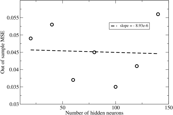
Figure 9: Plot of the observed out of sample MSE for SFP-MLE in the forecast of the NMR–laser time–series for increasing hidden layer size. The SFP parameters are selected in order to have a posterior density as sharp as possible. The out of sample errors appear to be independent of the neural network complexity.

A linear regression on the errors shows no evidence of an increment of the errors with the ANN size. A standard F-test for this regression indicates that the null hypotesis of a constant slope can’t be rejected at a $95\%$ confidence.

Number of hidden neurons	Predicted MSE	Out of sample MSE
20	0.058	0.049
40	0.062	0.053
60	0.047	0.037
80	0.057	0.045
100	0.058	0.035
120	0.060	0.041
140	0.064	0.056

Table 5: The observed out of sample MSE for the SFP ANN in the forecast of the NMR–laser time–series for increasing hidden layer size.

The number of loss function evaluations of a SFP sampling grows linearly with the potential’s dimension [Berrones, 2008]. Therefore, Table 5 indicates that SFP is capable to perform a correct estimation of the posterior density with a total number of loss function evaluations that grows linearly with system’s size. The evaluations of the potential function gives the major contribution to the computational cost. In Fig. 10 is presented the total computation time of each of the runs of Table 5.

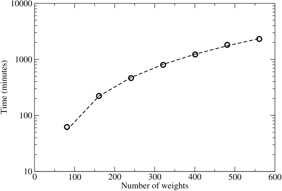
Figure 10: Dependence between computation time and ANN size for SFP-MLE training in the NMR–laser example. The SFP parameters are selected in order to have a posterior density as sharp as possible, which is computationally demanding. The dashed line represents the best quadratic fit, given by $Time=-26.57+0.46N-0.007N^{2}$.

The computation time grows slowly with the system’s dimension, which is consistent with the linear behavior predicted by SFP theory. This experimental result is important because it shows the value of SFP sampling for large scale systems. In the context of global optimization, it appears that SFP should be further adapted to alleviate at some extent the curse of dimensionality suffered by any stochastic optimization method in order to be competitive with the current best algorithms [Melchert & Hartmann, 2008]. However, Table 5 and Fig. 10 suggest that for density estimation purposes, the correct estimation of large dimensional densities via SFP sampling is a polynomial time computational procedure, with a total number of loss function evaluations that behave linearly. These properties may be valuable in other applications besides Bayesian inference, like for instance Monte–Carlo simulations of large physical systems.

5 Discussion

The framework for Bayesian learning based on SFP sampling introduced in this Letter is directly connected to equilibrium statistical mechanics. In particular, using a dimensionless Boltzmann constant $k=1$, it turns out that an entropy $S$ can be introduced,

$$S=-\int_{\vec{w}}p(\vec{w}|A)\ln p(\vec{w}|A)d\vec{w},$$ (26)

therefore obtaining the thermodynamic relation

$$\left<V(\vec{w}|A)\right>=S-\left<\ln p(A|\vec{w})\right>.$$ (27)

The exploitation of the link of SFP Bayesian learning with equilibrium statistical mechanics appears to be promising taking into account that SFP provides analytic expressions for the marginals, from which mean–field approximations to the quantities of interest may be derived.

An additional interesting research question is the study of more general forms of uncertainty affecting the stochastic search in the weight space. In this regard, it should be noticed that the SFP formalism is in principle not limited to the estimation of the stationary density of a diffusion on a potential under white Gaussian additive noise. Through the use of generalizations to the Fokker–Planck equation based on the expansion of the master equation, like for instance the Van Kampen expansion [Van Kampen, 1992], several other stochastic search processes may be considered. If the posterior densities resulting from such generalized processes are more adequate in some situations seems to be an appealing question to further study.

A techical issue in which there may be room for the improvement of the SFP approach regards the selection of the most appropriate basis function family for the approximation of the conditionals. In this Letter it has been used the Fourier basis only because of its simplicity, but in principle any other basis can be used.

Other relevant research line that follows from the results presented so far consists on the application of SFP learning to large and complex systems. If the observed polynomial behavior of computation time holds in general, it would be valuable to apply the SFP technique on very large inference models, taking advantage of the intrinsic parallel nature of the SFP sampling algorithm.

References

- [Auld, 2007] Auld, T., Moore, A. W. & Gull, S. F. (2007). Bayesian Neural Networks for Internet Traffic Classification IEEE Transactions on neural networks, 18(1), 223–239.
- [Badii et al., 1994] Badii, R., Brun, E., Finardi, M., Flepp, L., Holzner, R., Parisi, J., Reyl, C., & Simonet, J. (1994). Progress in the analysis of experimental chaos through periodic orbits. Rev. Mod. Phys. 66, 1389–1415.
- [Berrones, 2008] Berrones, A. (2008). Stationary probability density of stochastic search processes in global optimization. J. Stat. Mech., P01013.
- [Berrones, 2009] Berrones, A. (2009). Characterization of the convergence of stationary Fokker–Planck learning. To appear in Neurocomputing. doi:10.1016/j.neucom.2008.12.042
- [Canty, 1999] Canty A. (1999). Hypothesis Tests of Convergence in Markov Chain Monte Carlo. Journal of Computational and Graphical Statistics, 8, 93–108.
- [Celeux et al., 2000] Celeux, G., Hurn, M. & Robert, C. P. (2000). Computational and Inferential Difficulties with Mixture Posterior Distributions. Journal of the American Statistical Association, 95(451), 957–970.
- [Chib et al., 2002] Chib, S., Nardari, F. & Shephard, N. (2002). Markov chain Monte Carlo methods for stochastic volatility models. J. Econometrics, 108, 281–316.
- [Ghahramani & Beal., 2001] Ghahramani, Z. & Beal, M. J. (2001). Graphical Models and Variational Methods. In Advanced Mean Field Methods, 161–177. MIT Press.
- [Grasman & van Herwaarden, 1999] Grasman, J. & van Herwaarden, O. A. (1999) Asymptotic Methods for the Fokker–Planck Equation and the Exit Problem in Applications. Springer.
- [Jalobeanu et al., 2002] Jalobeanu, A., Blanc–Feraud, L. & Zerubia, J. (2002). Hyperparameter estimation for satellite image restoration using a MCMC maximum-likelihood method. Pattern Recognition, 35, 341–352.
- [MacKay, 1992] MacKay, D. J. C. (1992). A practical Bayesian framework for backpropagation networks. Neural Comput., 4(3), 448–472.
- [Malzahn & Opper, 2002] Malzahn, D. & Opper, M. (2002). Statistical Mechanics of Learning: A Variational Approach for Real Data, Phys. Rev. Lett. 89(10), 108302.
- [Marin et al., 2005] Marin, J.M., Mengersen, K. & Robert, C. P. (2005). Bayesian modelling and inference on mixtures of distributions. In Handbook of Statistics 25, D. Dey and C.R. Rao (eds). Elsevier-Science.
- [Marwala, 2007] Marwala, T. (2007). Bayesian training of neural networks using genetic programming Pattern Recognition Letters 28, 1452–1458.
- [Melchert & Hartmann, 2008] Melchert, O. & Hartmann, A. K. (2008). Ground states of 2D J Ising spin glasses obtained via stationary Fokker–Planck sampling J. Stat. Mech., P10019.
- [Nakajima & Watanabe, 2007] Nakajima, S. & Watanabe, S. (2007). Variational Bayes Solution of Linear Neural Networks and Its Generalization Performance Neural Comput., 19(4), 1112–1153.
- [Neal, 1996] Neal, R. M. (1996). Bayesian Learning for Neural Networks. Springer.
- [Ripley, 1994] Ripley, B. D. (1994). Neural networks and related methods for classification (with discussion). J. Roy. Statist. Soc. B 56, 409–456.
- [Risken, 1984] Risken, H. (1984) The Fokker–Planck Equation. Springer.
- [Roberts & Polson, 1994] Roberts, G. O. & Polson, N. G. (1994). On the Geometric Convergence of the Gibbs Sampler J. R. Statist. Soc. B 56 2, 377–384.
- [Roberts & Stramer, 2002] Roberts, G. O. & Stramer, O. (2002). Langevin Diffusions and Metropolis-Hastings Algorithms Methodology and Computing in Applied Probability 4, 337–357.
- [Kantz & Schreiber, 2004] Kantz, H. & Schreiber, T. (2004). Nonlinear Time Series Analysis. Cambridge University Press.
- [Van Kampen, 1992] Van Kampen, N. G. (1992). Stochastic Processes in Physics and Chemistry. Elsevier.
- [Weigend & Gershenfeld (Eds.), 1994)] Weigend, A. S. & Gershenfeld, N. A. (Eds.) (1994). Time Series Prediction: Forecasting the Future and Understanding the Past. Santa Fe Institute Studies in the Sciences of Complexity XV. Addison–Wesley.