Monte Carlo Simulations of Star Clusters - VI. The globular cluster NGC 6397

Abstract

We describe Monte Carlo models for the dynamical evolution of the nearby globular cluster NGC 6397. The code includes treatments of two-body relaxation, most kinds of three- and four-body interactions involving primordial binaries and those formed dynamically, the Galactic tide, and the internal evolution of both single and binary stars. We arrive at a set of initial parameters for the cluster which, after 12Gyr of evolution, gives a model with a fairly satisfactory match to the surface brightness profile, the velocity dispersion profile, and the luminosity function in two fields. We describe in particular those aspects of the evolution which distinguish this cluster from M4, which has a roughly similar mass and Galactocentric distance, but a qualitatively different surface brightness profile. Within the limitations of our modelling, we conclude that the most plausible explanation for the difference is fluctuations: both clusters are post-collapse objects, but sometimes have resolvable cores and sometimes not.

1 Introduction

This is the third paper in which we aim to construct a dynamical evolutionary model of a specific Galactic globular cluster, following $\omega$ Cen (Giersz & Heggie, 2003) and M4 (Heggie & Giersz, 2008). We are motivated by a variety of questions: How did globular clusters come to be as they are? What was the initial mass function of their stars, and the abundance of their binaries? Where should we look for signs of the dynamical evolution of their binary population?

So far, our most interesting finding concerned M4, where we were surprised to find that our model had exhibited core collapse about 4Gyr ago, even though this cluster is not a classic core collapse cluster, to judge by its surface brightness profile (Trager et al., 1995). Now we turn to an object which is almost the twin of M4, i.e. the southern globular cluster NGC6397. As we shall see in Sec.2 these two clusters have much the same mass, Galactic orbit, binary fraction, etc. The one feature where they differ strikingly is the surface brightness profile: NGC6397 does exhibit a collapsed core. Because of their other similarities, conventional explanations for this difference are untenable. In this paper our chief aim is to provide a plausible explanation of this contrast between these two clusters.

Our technique is fundamentally a Monte Carlo simulation method in a style originally devised by Hénon (1971), but developed afresh by Giersz (1998, 2001, 2006), partly following ideas developed by Stodołkiewicz (1982, 1986). It now incorporates all the main processes affecting the long-term evolution of globular star clusters, including the Galactic tide and the internal evolution of single and binary stars, not to mention dynamical interactions between these populations. It has been tested against results of $N$-body simulations of the rich open cluster M67 (Giersz, Heggie, & Hurley, 2008), and at present such a code is an unmatched tool for the evolutionary modelling of globular clusters.

This is by no means the first time dynamical models have been constructed for this cluster. Almost all previous modelling, however, was concerned with the construction of an equilibrium model, such as a King model. Such models do not readily lend themselves to consideration of dynamical evolution. Exceptions are the $N$-body models described in Richer et al. (2008); Hurley et al. (2008); Davis et al. (2008a) and the Fokker-Planck modelling of Drukier (1993, 1995). Together with our Monte Carlo method, these techniques offer three ways in which the effects of dynamical evolution on a globular cluster may be assessed.

The $N$-body models are essentially free of simplifying dynamical assumptions, except that a globular cluster like NGC6397 is too rich for its entire evolution to be modelled directly. Therefore assumptions are needed when $N$-body models are applied to such objects. For example, Richer et al. (2008) and Hurley et al. (2008) observe that a particular $N$-body model, at an age of 16Gyr, has a mass function which conforms approximately to that observed in a certain field in NGC6397, though the model has a mass at 16Gyr of only about $10^{4}M_{\odot}$, which is considerably smaller than estimates for this cluster (Tables 1, 4). As these authors emphasise, their $N$-body model is not a model of NGC6397, but is intended to allow estimates of the effect of dynamical evolution on the spatial distribution of binaries, and so on.

The Fokker-Planck models of Drukier (1995) are essentially scale-free, but the paper includes an exhaustive discussion of how the scales and initial parameters of the models are constrained by fitting to profiles of surface density and velocity dispersion, and to ground based mass functions at three radii.

Our own approach combines some of the advantages of $N$-body and Fokker-Planck techniques. Similar to Drukier’s, our aim is to construct a dynamical evolutionary model which provides a satisfactory fit to surface brightness and velocity dispersion profiles, and to luminosity functions. But our method of simulation is a star-by-star method, like the $N$-body technique, and it shares with Hurley et al. (2008) the use of synthetic modelling of the internal evolution of both single and binary stars. Our advantage over the $N$-body modelling is the use of a realistic number of particles (which depends in turn on speed of computation), and our advantage over the Fokker-Planck treatment is the inclusion of binaries, and better stellar evolution. Our principle disadvantage, compared with the $N$-body modelling, is the need for simplifying assumptions in the treatment of dynamical encounters of all kinds; compared with the work of Drukier (1995), our main shortcoming is our very limited ability to assess the uniqueness of the model we eventually arrive at.

In the following section we summarise some global data about NGC6397 and its close relative, M4. We also describe the data which we use in assessing our models, so that they match various aspects of the cluster at the present day. Next we describe our best models, and include an assessment of the reasons why the two clusters have such dissimilar surface brightness profiles. In the final section we sum up and discuss aspects of our initial conditions more generally.

2 Data on NGC 6397

Global data relevant to our study of NGC6397 is listed in Table 1, along with data for M4, for comparison. In most cases the sources given are not the original sources; nevertheless some of the sources include discussion of the literature and of the data selected. We became aware of the age determination given in this table only after our research was well under way, and compare our model at an age of 12Gyr, as we did for M4.

Table 1: Data on NGC6397 and M4 (NGC6121)

	NGC6397	M4
$R_{GC}^{1}$ (kpc)	6.0	5.9
${R_{\oplus}}^{2}$ (kpc)	$2.55^{5}$	$1.72^{3}$
$A_{V}$	$0.56^{4}$	$1.33^{3}$
$(m-M)_{V}$	$12.03^{4}$	$11.18^{3}$
$[Fe/H]^{1}$	-1.95	-1.20
$M_{V}^{1}$	-6.63	-7.20
$M(M_{\odot})$	${}^{6}6.6\times 10^{4}$	${}^{3}6.25\times 10^{4}$
$r_{c}$ (arcmin)1	0.05	0.83
$r_{h}$ (arcmin)1	2.33	3.65
$r_{t}$ (arcmin)1	15.81	32.49
Age (Gyr)7	$11.47_{-0.47}^{+0.47}$	$12.1_{-1.8}$

Sources and notes: ¹ Harris (1996); ² Distance from earth; ³ Richer et al. (2004); ⁴ Richer et al. (2008); ⁵ from $m-M$; ⁶ Drukier (1995); ⁷ Hansen et al. (2004, 2007)

For the surface brightness our main source, as with M4, has been Trager et al. (1995), but we have also considered the HST profile of the central parts of the cluster of Noyola & Gebhardt (2006). These are in reasonable agreement where they overlap, except at the very centre, where the HST profile is slightly brighter. To some extent the agreement is artificial, as Noyola & Gebhardt calibrated their surface brightness determinations against the older data.

The velocity dispersion profile given by Meylan & Mayor (1991) is based on radial velocities of 127 stars. We have also been kindly given access to a catalogue of unpublished radial velocities of over 1400 stars observed by the Padova group (G. Piotto, pers.comm.). The reduction of this data is not yet complete, however, and we have made no use of them here.

While there is no shortage of luminosity functions in the literature for NGC 6397, relatively few of these are properly normalised, i.e. give counts in a stated area of sky. All too often only the shape of the luminosity function has been published. Our primary sources of absolute luminosity functions are restricted to

1. Paresce, de Marchi, & Romaniello (1995), who give counts in the F814W band in a field about 4.6 arcmin from the cluster centre; and

2. Mould et al. (1996), who gave similar results for a field at about 10 arcmin.

For purposes of comparison with our models, which give $I$-band magnitudes, we have ignored the difference between $m_{I}$ and $m_{814}$. From the models tabulated in Baraffe et al. (1997) we estimate that the effect of this on the luminosity function is less than 5%.

Finally we mention the observed binary fraction. From the binary sequence in the colour-magnitude diagram, Davis et al. (2008a) conclude that this decreases from about 5% at the centre to about 1% at 5 arcmin. On the other hand A. Milone (pers. comm.) estimates that the outer binary fraction is about 3-4%, rising to about 9% in the inner 15 arcsec. Clearly, there is some uncertainty here. For later discussion, these results are presented, along with similar information for M4, in Table 2.

Table 2: Approximate observed binary fractions in NGC6397 and M4

M4	M4	NGC 6397	NGC 6397	Source
centre	off-centre	centre	off-centre
10%	–	9.2%$\pm$3.0	3.7%$\pm$0.8	$a$
2%	1%	5.1%	1.2%	$b$

Sources: $a$ Milone et al. (2008) and Milone, pers.comm. ; $b$ Richer et al. (2004, M4), Davis et al. (2008a, NGC 6397)

3 Models of NGC 6397

3.1 The search for a model

Our general approach is to follow a cycle in which we (a) specify a model, (b) follow its evolution with the Monte Carlo code, (c) compare with observational data on surface brightness and velocity dispersion profiles, and luminosity functions and (d) alter the initial model to improve the fit. Though complete models of NGC6397 now take only about a day on a good PC, thanks to recent software improvements, we still try to accelerate the first few cycles by using scaled-up results from smaller models (Heggie & Giersz, 2008). From the same source we list in the first column of Table 3 the free parameters which we have to adjust in step (a) of each cycle, except that the total mass $M$ is determined by the other parameters.

Table 3: Initial parameters for models of NGC6397, and ranges sampled

Number of stars, $N$	$4\times 10^{4}$	$10^{5}$	$5\times 10^{5}$
Mass, $M$
Tidal radius, $r_{t}$ (pc)	[66.2:80.9]	[56.0:61.9]	[40]
Half-mass radius, $r_{h}$	$r_{t}$/[60:100]	$r_{t}$/[95:105]	$r_{t}$/[60:105]
Binary fraction, $f_{b}$	[0.03:0.09]	[0.06:0.09]	[0.03:0.15]
Slope of the lower IMF, $\alpha$	[0.7:1.3]	[0.7:1.0]	[0.3:1.1]

Since the present-day parameters of NGC 6397 are quite similar to those of M4 (Table 1), we started close to the parameters which we had reached for M4 in Heggie & Giersz (2008). Our scaled-down models with $N=40000$ and $100000$ stars coarsely covered the ranges stated in the second and third columns of Table 3. This information requires some explanation. First, we have not stated the corresponding total mass $M$; as we have said, this is determined from the other stated parameters ($N,f_{b}$ and $\alpha$) for our choices of the initial mass functions of single stars and binaries, and the distribution of binary component ratios. Second, the ranges of tidal radius $r_{t}$ look disjoint, but scaling by $N$ also requires scaling lengths, in order to keep the relaxation time fixed (see Heggie & Giersz (2008)). Also, we often internally used equivalent values for $N=10^{4}$, which explains the odd choices listed here. Third, we specified our initial half-mass radius in terms of the ratio $r_{t}/r_{h}$, which explains the way in which we have expressed $r_{h}$. Finally, each model can be scaled (approximately) to a different value of $N$, and we have not recorded the ranges with which we experimented.

By comparing these models (by eye) with the observational data we have mentioned, we located a promising region in this parameter space. This was then explored with a full-sized model over parameter ranges given in the fourth column of the Table. This exploration was less systematic, however, and not all combinations of parameters were considered. Also, we extended somewhat the ranges of $f_{b}$ (the binary fraction) and $\alpha$ (the power law index of the lower initial mass function), as indicated.

Before we describe one of our best models in detail, we record here the effect of departing significantly from these apparently near-optimal values of the parameters.

1. $N$: this can be explored (approximately) by scaling, which leads to the following conclusions. A 25% increase in $N$ leads to an overall increase in the surface brightness by about 0.4 magnitudes, an overall increase in the velocity dispersion profile (i.e the root mean square line-of-sight velocity) by about 15%, and an increase in the luminosity functions by about 30%. Note that the scaling we employ preserves the relaxation time, and so lengths are scaled as well as $N$ itself (Heggie & Giersz, 2008).

2. $r_{t}$: an increase by 10% causes little change in the surface brightness profile except above about $0.5r_{t}$, where it causes an approximately proportional spatial extension of the profile. An increase by 10% causes approximately the same percentage increase in the velocity dispersion, and large increases in the luminosity function: by factors of approximately 2 and 3 in the inner and outer fields, respectively.

3. $r_{h}$: A 10% increase causes a slightly less concentrated surface brightness profile, changing the surface brightness by only a few tenths of a magnitude. It produces about a 3% decrease in the velocity dispersion profile, and decreases in the luminosity functions by about 20%.

4. $f_{b}$: A doubling of the primordial binary fraction (from 0.03 to 0.06) has no discernible effect on the surface brightness profile or the luminosity functions, and only a small (of order 2%) increase in the velocity dispersion.

5. $\alpha$: An increase in the power-law index of the lower initial mass function by 0.3 results in a decrease in the surface brightness by about 0.2–0.3 magnitudes, and a decrease in the velocity dispersion profile by about 8%. The luminosity function is almost unchanged at the bright end, but increases by about 25% at the faint end.

In considering these remarks, it must be remembered that they refer to the range of radii and magnitudes for which we had observational data, which are displayed in Figs.1–5. This helps to explain why an increase in the tidal radius can have a much larger effect on the luminosity function than on the surface brightness, because these refer essentially to fainter and brighter stars, respectively. An increase in tidal radius causes less loss of low-mass stars, and so it can be understood qualitatively how the stated changes in the various observational parameters arise, when $r_{t}$ is increased.

The above remarks also show that some parameters are much more easily determined than others. The binary fraction is best determined by comparison with the observed binary fraction (Table 2), and is very poorly constrained by the surface brightness and velocity dispersion profiles, and the luminosity function. On the other hand the effect of $r_{t}$ on the luminosity function is so great that it is well determined (for given values of the other parameters). Of the remaining three parameters we judge that $\alpha$ is the least well determined.

Eventually this exploration led to a small number of satisfactory models, one of which is summarised in Table 4. There we show for comparison the corresponding results from the most satisfactory model of M4, and a few interesting numerical results. The binary fraction needs some explanation, as it appears there has been much more depletion in the model of NGC6397 than in the model of M4. The reason for this is that the M4 model used a uniform initial distribution of semi-major axis, while study of the radial velocity binaries in M4 detected by Sommariva et al. (2008) has suggested to us that a better fit is provided by models with the semi-major axis distribution given by the procedure described by Kroupa (1995). This gives a higher proportion of soft binaries, and hence enhanced destruction.

Since carrying out this search for a model, we have also codified an extensive grid of small scale models in such a way that initial values can be found as a function of corresponding values at the present day. This does not, however, fully solve the problem of determining initial conditions, as present-day values of these parameters are not often known reliably, and a fit to values drawn from the literature does not guarantee a fit to an entire surface brightness profile, etc. Nevertheless, this procedure may in future provide plausible starting values for a more refined search.

Table 4: Initial and final conditions for models of NGC6397 and M4

	NGC6397: 0Gyr	NGC6397: 12Gyr	M4: 0Gyr	M4: 12Gyr
Mass ($M_{\odot}$)	$3.65\times 10^{5}$	$6.03\times 10^{4}$	$3.40\times 10^{5}$	$4.61\times 10^{4}$
Luminosity ($L_{\odot}$)	$5.1\times 10^{6}$	$3.40\times 10^{4}$	$6.1\times 10^{6}$	$2.55\times 10^{4}$
Binary fraction	0.090	0.044	0.07	0.057
Slope of the lower mass function	1.1	0.48	0.9	0.03
Mass of white dwarfs ($M_{\odot}$)	0	$2.74\times 10^{4}$	0	$1.81\times 10^{4}$
Mass of neutron stars ($M_{\odot}$)	0	$3.14\times 10^{3}$	0	$3.24\times 10^{3}$
Tidal radius (pc)	40.0	22.0	35.0	18.0
Half-mass radius (pc)	0.40	3.22	0.58	2.89
Core radius1 (pc)	0.22	$0.041\pm 0.012$	0.31	$0.043\pm 0.017$

¹The definition is given in the caption of Fig.7. For 12Gyr the values stated are the mean and 1-$\sigma$ variations over the period 11–12Gyr. For 0Gyr the value uses the same formula, but analytic values for the central density and velocity dispersion.

3.2 The surface brightness profile

Figure 1: Surface brightness (in units of V magnitudes per square arc second) as a function of projected radius (arc seconds), in the model and in the observational data from Trager et al. (1995) and Noyola & Gebhardt (2006). Only the data classed by Trager et al as of highest weight are included. Several model profiles are given, corresponding to various limits on the brightest star included. The profiles for $10^{3}$ and $10^{2}L_{\odot}$ differ little.

Fig.1 shows how the surface brightness profile of our model compares with the ground-based data of Trager et al. (1995) and the HST data of Noyola & Gebhardt (2006). Except at small radii, the model is slightly faint compared with the former, which in turn is fainter than the latter. The model is especially faint, and too small, at large radii, but we have explained in Giersz, Heggie, & Hurley (2008) that this is an artifact of our treatment of the tide.

Next we should explain the reason for the peaks in the model surface brightness profile, which are particularly obvious at small radii. The Monte Carlo code gives the radius and V-magnitude of each star, and, in order to construct the surface brightness, we represent each star by a sphere of the corresponding radius and magnitude. The projected surface brightness of a sphere is infinite at its edge, and the peaks occur at projected radii close to the radii of stars, especially bright ones. From an observational point of view also the surface brightness has very large fluctuations (at the locations of the stars), and these are reduced by averaging over annuli, exclusion of bright stars, etc.

The effect of excluding bright stars in the model is shown in Fig.1 by four profiles in which successively fainter bright stars are excluded, down to roughly the turnoff. As expected, the overall level and fluctuations are reduced, but these plots do little to clarify the nature of the core in the model. When the fluctuations are sufficiently suppressed, the profile is severely biased.

Another way of suppressing fluctuations, i.e. smoothing in radius, is illustrated in Fig.2, which focuses on the inner part of the cluster. The most noticeable difference between the various profiles is, once again, the fact that the profile of Noyola & Gebhardt (2006) is somewhat brighter at most radii.

Figure 2: Surface brightness (in units of V magnitudes per square arc second) as a function of projected radius (arc seconds), in the inner part of the cluster. For the model, various smoothed profiles are shown, and the key states the number of intervals, evenly spaced in $\log R$, over the interval plotted in Fig.1. The bin sizes in $\log R$ are 0.037, 0.074 and 0.185, respectively. The observational data are as in Fig.1. The curve labelled “NS kicks” is discussed in Sec.3.6.

Noyola & Gebhardt (2006) give a short but interesting review of the literature on the surface brightness profile of NGC6397, and point out that, despite its status as a collapsed core cluster, various authors have given core radii of order a few seconds of arc. Part of the reason for the difficulty of classifying the cluster may be gleaned from the $V$ surface brightness map given by Auriere, Lauzeral, & Ortolani (1990). The area within 7 arcsec of the centre is dominated by a roughly linear group of blue stragglers, and it is not clear how this influences a radially averaged profile.

The difficulties with the observational material are not confined to the centre, however. It is evident from Fig.2 that, even though this includes only material regarded by Trager et al as of highest weight, there are regions within the range 10–100 arcsec where their data is not self-consistent. In particular there is a “bump” around 40 arcsec (or possibly a trough at smaller radii) which could be fitted only by a highly contrived model. It is important to note also that the data of Noyola & Gebhardt is calibrated with the aid of the older data, by matching the integrated light of the newer data to the integral of a smooth fit to the older data.

We shall see in Sec.4.1 that the profile of the model is subject to considerable fluctuations, both in time and for different realisations of the same model. Therefore the question of whether the model is in agreement with the observational profile, even if the latter were completely reliable, has to be formulated statistically; in other words, can the observational profile be rejected as a member of the ensemble of profiles provided by the model, or not? We do not answer this question in this paper, but in this spirit we do provide a discussion in terms of the central surface brightness in Sec.4.1.

There is another way of approaching the question of whether the surface brightness profile of the model matches that of NGC6397, at least qualitatively, and that is to ask whether our model would be taken for a collapsed-core cluster. Even the most smoothed model profile in Fig.2 is not monotonic, but all suggest that this is a model of a cluster which would be classified as having a cusped profile rather than a cored one. Note that, while we have not attempted any quantitative measure of this statement, to some extent we have here followed the lead of Trager et al. (1995), who classified the observed profiles of star clusters apparently without any numerical criterion for doing so.

3.3 Velocity dispersion profile

The purpose of Fig.3 is to illustrate the satisfactory fit between the line-of-sight velocity dispersion of the model and the observational data of Meylan & Mayor (1991). Only stars brighter than $M_{V}=7$ are included, as the observations are confined to giants and subgiants. In the model, binaries are represented by the velocity of their centre of mass; internal motions are neglected. The slight depression in the velocity dispersion near the centre may be attributable to mass segregation; similar qualitative features occur in the more idealised models of Chernoff & Weinberg (1990). No such central inversion in the velocity dispersion was noticeable in our models of M4 (Heggie & Giersz, 2008), however, and this may be associated with the fact that the radius of the central concentration of heavy remnants in our model of NGC 6397 is somewhat smaller than in our model of M4. (Note that, in both models, neutron stars and white dwarfs receive no natal kick.)

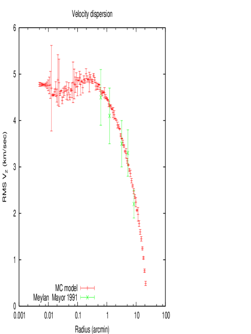
Figure 3: Line-of-sight velocity dispersion (km/sec) as a function of projected radius (arc min) for the Monte Carlo model, and from the observational data of Meylan & Mayor (1991).

3.4 Luminosity functions

Main sequence luminosity functions are displayed, for the model and two observational data sets, in Figs.4 and 5. For the model, we counted all objects in the colour-magnitude diagram above a line just below the main sequence. These luminosity functions therefore include unresolved binaries (in the same way that these were not removed from the observational data with which we compare).

While the surface brightness profile (Fig.1) gives the impression that the model is slightly faint at most radii, the model luminosity functions generally seem somewhat too high, are not steep enough at the bright end, and peak at somewhat fainter magnitudes (compared with the observational data.) These discrepancies seem quite recalcitrant; considerable experimentation with the initial conditions of the models has been unable to improve this aspect of the comparison with observation, though it has to be noted that, as far as the IMF is concerned, we have limited ourselves to varying the slope of the lower mass function. (The break in the slope of the assumed mass function occurs at $0.5M_{\odot}$, corresponding to about $M_{I}=6.9$.) In any event it must be remembered that the observational data are affected by incompleteness, especially at the faint end in the inner field. Furthermore, Mould et al. (1996) show that independent counts in the inner field at the bright end may differ by as much as 30%. Finally, while the model luminosity functions correspond to the stated radius, the observational luminosity functions are determined in fields which cover a range of radii, and stellar densities. Our experience is that the overall fit to the luminosity function depends sensitively on some of the initial parameters of our models (Sec.3.1), and so we regard the agreement achieved with our model as not unsatisfactory.

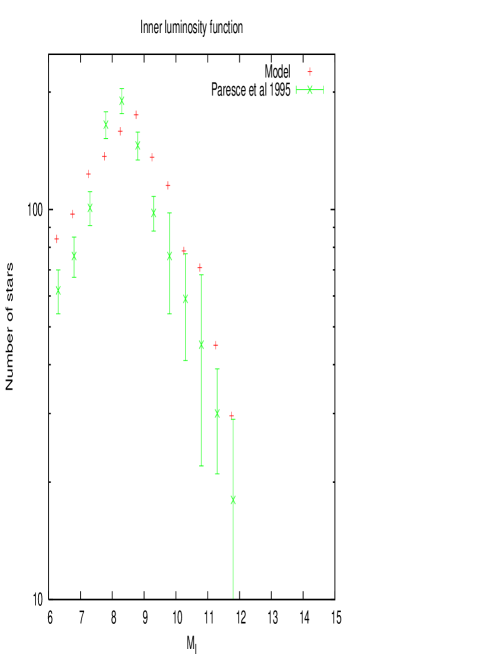
Figure 4: I-band luminosity function in a field at a radius of about 4.6 arcmin (Paresce, de Marchi, & Romaniello, 1995) compared with the model. Strictly the observational magnitude is $M_{814}$.

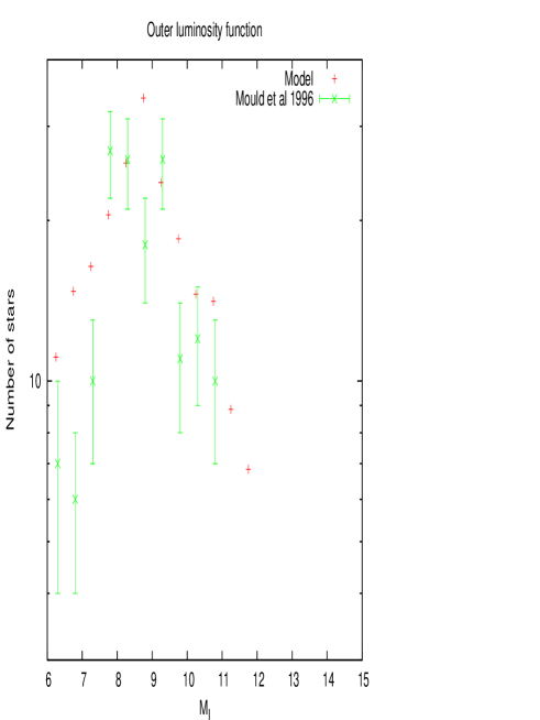
Figure 5: I-band luminosity function in a field at a radius of about 10 arcmin (Mould et al., 1996) compared with the model.

3.5 Binary fraction

We have already mentioned the difficulty in assessing observationally the binary fraction in this cluster. As for the model, the result depends on whether we include all objects, including white dwarfs, or only objects on or above the main sequence (Fig. 6). For the latter, the binary fraction drops rapidly with increasing radius, roughly in qualitative agreement with the observational results (Table 2). We assume that it would be equally easy to produce a model in rough quantitative agreement, simply by reducing the initial binary fraction in the model. Our reason for presenting results using an excessive binary fraction is that we wanted to address the question of whether it is the binary fraction which determines whether a post-collapse cluster exhibits a cusped or cored profile (Sec.5.2.2). We already see that this is not the case: here we have a model with a non-King surface brightness profile but an excessive binary fraction.

Figure 6: Projected cumulative binary fraction for all objects and for objects on or above the main sequence. The ordinate is the binary fraction for all objects with projected radius less than the value on the abscissa. In computing this fraction for objects on or above the main sequence, both numerator and denominator exclude white dwarfs and other degenerate objects.

3.6 Neutron star kicks

One of our aims in this paper (Sec.4) is to compare our modelling of the two clusters M4 and NGC6397. Therefore we have in general adopted similar astrophysical assumptions for NGC6397 as for M4 in Heggie & Giersz (2008). (One exception is the initial distribution of binary periods, but it has already been mentioned that this has little discernible effect on the fit to the observational data shown in Figs.1–5.) In our modelling of M4 we gave no natal kicks to neutron stars, and have adopted the same assumption here. Though there are grounds for considering that neutron stars may indeed be born with low kick velocities (e.g. Pfahl, Rappaport, & Podsiadlowski 2002), we here consider one model with a more conventional kick distribution, with a one-dimensional velocity dispersion of 190km/s.

We did not attempt to iterate on the initial parameters to optimise the fit with the observational data, but used those given in Tab.4. In the resulting model the time of core collapse was delayed by about 4Gyr to 9Gyr, and by 12Gyr the mass of neutron stars was smaller by a factor of about 20. Nevertheless the model exhibited a velocity-dispersion profile and luminosity functions very similar to those of the model with no neutron star kicks (Figs.3–5), including the imperfections of the latter. The main difference was in the surface brightness profile, the central part of which is displayed in Fig.2. This generally matches the data of Noyola & Gebhardt (2006) better than our standard model, but not in the innermost 1 or 2 arcsec, and it has the character of a King-like profile with a small core. Therefore, while a model with neutron star kicks may be a better basis on which to optimise over the initial parameters, it does not of itself provide an explanation for the non-King profile of NGC6397.

4 Comparison of M4 and NGC 6397

What is striking about Table 4 is the similarity of the initial conditions for these two clusters, and yet one (M4) is described traditionally as a ‘King-model’ cluster, while the other (NGC 6397) is classified as ‘post-core-collapse’ (Trager et al., 1993). As we have seen (Sec.3.2) the observed surface brightness profile of NGC 6397 is not entirely unambiguous in this respect, while the similarities between the two clusters were further strengthened by Heggie & Giersz (2008), whose model of M4 suggested that this cluster experienced core collapse at an age of about 8Gyr. (Our model of NGC6397 is also post-collapse, the collapse of the core having ended at a somewhat smaller age of 5Gyr; see Fig.7.)

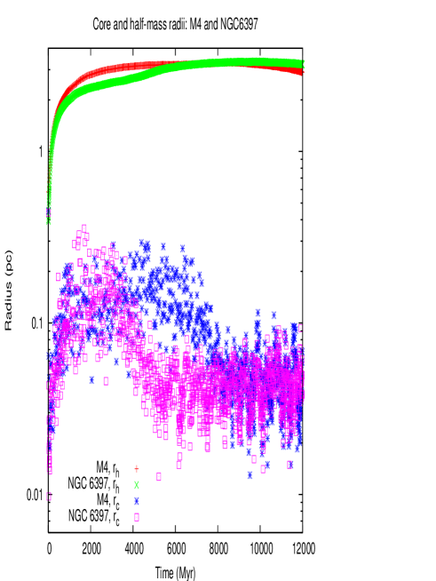
Figure 7: Evolution of the half-mass and core radii of our models of NGC 6397 and M4. Note that what is plotted here is the dynamical core radius, which is computed by the formula $r_{c}^{2}={3\langle v^{2}\rangle}/({4\pi\rho_{0}}),$ where the mass-weighted mean three-dimensional velocity $\langle v^{2}\rangle$ and the central density $\rho_{0}$ are calculated for the innermost 20 stars.

The distinction between the two clusters on the basis of the observed surface brightness profile is, nevertheless, striking (Fig.8). Only slightly less striking is a similar comparison of the model surface brightness profiles (Fig.9). The availability of these models allows us to investigate, and even experiment with, the possible reasons for the difference between these clusters. Note that there are two questions: why the two clusters differ, and why the models of the two clusters differ. We approach the second question in this section. Mechanisms which can account for differences in the models may help to account for the differences in the actual clusters, but there are additional issues which may come into play in reality, and some of these are addressed in the final section of the paper.

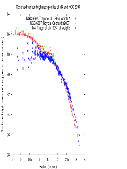
Figure 8: Observational surface brightness profiles of M4 and NGC 6397. For NGC 6397 only the data of highest weight (in the estimation of Trager et al. (1995)) are included.

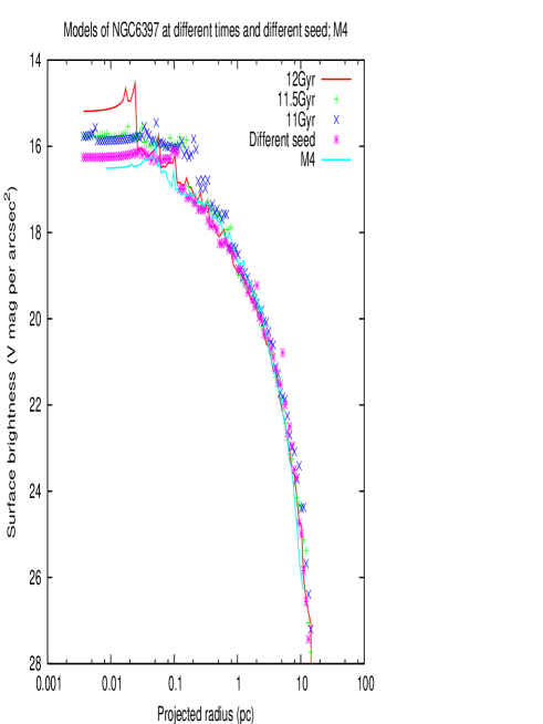
Figure 9: Surface brightness profiles of a model of NGC 6397 at ages of 11, 11.5 and 12 Gyr, and a second model with a different initial seed at 12 Gyr. Also shown is a model of M4 (Heggie & Giersz, 2008). Because the comparison involves different clusters, the surface brightness of the models has not been corrected for extinction, and the units of the radius are parsecs.

4.1 Fluctuations

One possible explanation for the difference between the models of the two clusters is fluctuations, and this hypothesis falls into at least two subclasses. First, we may suppose that, because of the motions of the stars, or possibly the occurrence of core oscillations (Sugimoto & Bettwieser, 1983), the profiles at different times will naturally differ. A second possibility is that different realisations of the same initial conditions could give rise to significantly different surface brightness profiles. We consider these two possibilities in turn.

4.1.1 Fluctuations in time

Fig.9 shows surface brightness profiles of a Monte Carlo model of NGC 6397 at three successive times separated by 500Myr. While one might expect to see a trend for the central surface brightness to decrease, this is obscured (in the present example) by fluctuations, which actually lead to an increase in the central surface brightness with time. Though we have plotted only three profiles from this model, they give the impression that fluctuations could be sufficient to account fully for the difference between the surface brightness profiles of our models of the two clusters M4 and NGC 6397: Fig.9 also displays the surface brightness profile of our model of M4 (Heggie & Giersz, 2008), plotted to the same physical length scale, and with all profiles uncorrected for extinction.

While the small number of profiles plotted in Fig.9 may be no more than suggestive, a more complete picture is provided by the evolution of the central surface brightness (Fig.10). Though the mean central surface brightness at the present day may be slightly larger for NGC6397 than for M4, any such difference is obscured by fluctuations. Indeed the fluctuations are large enough that the centre of NGC6397 is often dimmer than the centre of M4. Guided by Fig.9 this would imply also that it often has the less compact core. These results imply that it is no more than an accident that, at the present day, NGC6397 presents a cusped profile, while the profile of M4 is classified as cored.

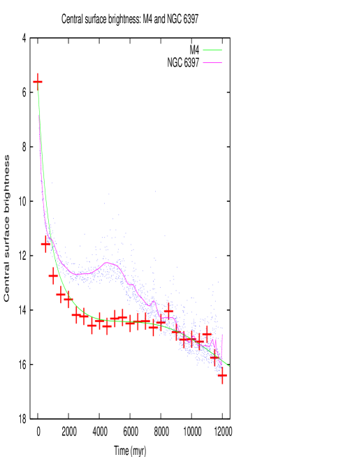
Figure 10: Evolution of the central surface brightness (in units of V magnitudes per square arcsec) of our models of NGC 6397 and M4. The smoothed curves are distorted by the large values at $t=0$, but elsewhere they are a satisfactory guide. The data are not available at the same frequency in the two models, but since the M4 model has been published, we did not attempt to rerun it.

As explained in the caption to Fig.10, we do not have data on the central surface brightness of our M4 model at the same frequency as for NGC 6397. We have, however, run a similar model of M4, and it confirms (Fig.11) that the distribution of central surface brightness is almost indistinguishable between the models of the two clusters, at least at the present day. (Fig.10 shows that the model of NGC6397 will have been brighter at earlier ages.)

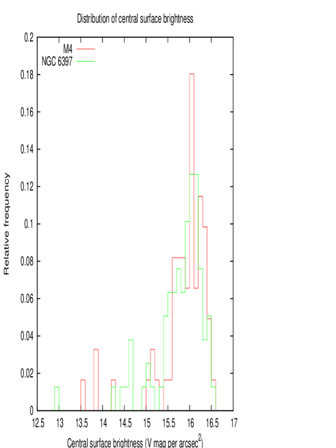
Figure 11: Histogram of the values of the central surface brightness in the models of M4 and NGC6397 between 11.6 and 12 Gyr.

The central surface brightness of our model at 12Gyr is 15.2 (uncorrected for extinction), and it can be shown from the data used to plot Fig.11 that this value is exceeded (i.e. the centre is brighter) about 14% of the time. While this may seem to imply that a surface brightness profile like that of NGC6397 is slightly unusual, it must be remembered that NGC6397 is itself actually slightly dimmer at the centre than our model, and so the proportion of models exhibiting a non-King profile may well exceed 14%. Furthermore, this percentage depends somewhat sensitively on the overall brightness of the model, which we know is slightly dim (Sec.3.2), and on the dynamics of the degenerate population (Sec.3.6).

4.1.2 Fluctuations between different realisations

What we have in mind here is not simply the fact that the masses and positions of stars will be different in different realisations, i.e. runs carried out with different seeds for the random number generator. More interesting is the possibility that the behaviour of a population of rare objects, present in sufficiently small numbers to be subject to large statistical fluctuations, could have a dramatic effect on the entire system. An example of this is Hurley’s important discovery of the effect of binary black holes (Hurley, 2007). He considered two different realisations of the same $N$-body model, which had $N=10^{5}$ single stars initially, with a mass spectrum and stellar evolution. In one of these realisations, a stellar-mass black hole binary happened to form dynamically, and it had a dramatic effect on the evolution of the core radius. Towards the end of the simulation, the core radius was about twice the value in the other realisation, where, by chance, no black hole binary was formed. Though black holes are expelled in our models at about the time of core collapse (Fig.7), and though our models are richer than Hurley’s, this process is indicative of the kind of fluctuations we have in mind.

Two realisations of the same model are shown in Fig.9, and they illustrate the fact that different realisations lead to more modest variations in the surface brightness profile than the variations (due to the presence or absence of a binary black hole) found by Hurley. Indeed, further study shows, not surprisingly, that the fluctuations between models with different seeds are comparable with those in time within one model (Figs.9,11).

As a cautionary remark, we should point out that the behaviour of fluctuations in a Monte Carlo model could, in principle, differ from their behaviour in an $N$-body model, though we have no reason to suspect this. The point is that, though we have been to considerable pains to ensure that the evolution of the total mass and various other parameters behaves similarly in our Monte Carlo models and in comparable $N$-body models (Giersz, Heggie, & Hurley, 2008), we did not check that fluctuations also behave similarly. In principle, each time some new feature is studied with a Monte Carlo model, it should be validated with a check against a model with fewer simplifying assumptions. In a forthcoming paper we shall present a comparison between our Monte Carlo model of NGC6397 and the evolution of an $N$-body realisation of the same model.

4.2 Different initial and boundary conditions

4.2.1 Different initial concentration

We already drew attention (Heggie & Giersz, 2008) to the high initial concentration of our model of M4, and our initial model of NGC6397 is even more compact. (The initial half-mass radii are given in Table 4.) It is tempting to suppose naively that the effect of this is a more concentrated configuration at an age of 12 Gyr, and that this alone is the explanation of the difference between the surface brightness profiles of the two clusters. We have already mentioned, however, that the fluctuations in the central surface brightness are much larger than any systematic difference; it is only earlier in the evolution of these clusters that NGC6397 was systematically brighter than M4. The evolution of the half-mass radius is also generally very similar for both clusters (Fig.7), even though initially the half-mass radius of our model of M4 was almost 50% larger than that of the model of NGC6397.

One can see systematic differences in the two clusters by study of the central escape speed, which in our model of NGC 6397 always exceeds that in our model of M4 (Fig.12). The reason why these differences are more apparent is that fluctuations in the core have a much smaller effect on the central escape speed than on the central surface brightness, as so much of the central potential is determined by the total mass and half-mass radius of the cluster.

The higher initial concentration should lead to enhanced destruction of binaries, but the overall binary fraction is low enough that this difference has no discernible effect on the surface brightness profile.

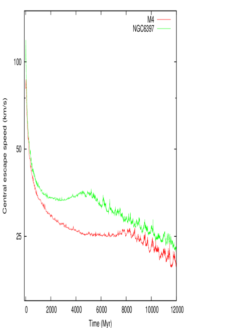
Figure 12: Evolution of the central escape speed in our models of NGC 6397 and M4. The ordinate is logarithmic.

4.2.2 Other factors

While we have attributed the systematic differences in the two curves in Fig.10 to the initial concentration, there are several other differences between the initial conditions of the models depicted (Tab.4). But tests have shown that, if we vary each initial condition one at a time, all have a minor effect on the evolution of the central surface brightness, except for the initial concentration. In particular, changing the binary fraction has little effect compared with the difference of initial half-mass radius.

5 Conclusions and Discussion

5.1 Conclusions

We have constructed a dynamical evolutionary model for the Galactic globular cluster NGC 6397. The model is based on a Monte Carlo treatment of dynamical interactions (2-, 3- and 4-body), and synthetic treatments of the evolution of single and binary stars. By varying a number of initial parameters ($N$, tidal and half-mass radii $r_{t}$ and $r_{h}$, binary fraction, slope of the lower IMF; see Tables 3, 4) we have constructed a model which, after 12Gyr of evolution, resembles NGC 6397 in terms of the surface brightness profile, the velocity dispersion profile, and the luminosity function at two radii.

Like the clusters themselves, our model for NGC 6397 has a higher central surface brightness than the model for M4, which is associated with the fact that, while M4 has a surface brightness profile resembling a King model, NGC 6397 has a more compact central profile which has led to its classification as a non-King cluster. Though this is associated in the literature with the distinction between pre- and post-collapse clusters, we find that both clusters are in the post-collapse phase of evolution. Fluctuations are the dominant mechanism responsible for the different brightness profiles.

5.2 M4 and NGC6397

We have just summarised the main reason why our models of these two clusters have distinctively different surface brightness profiles. But we pointed out in the previous section that this is not the same as explaining why these two clusters have different profiles, partly because there are so many aspects of their structure and evolution which we have not considered in our modelling. Here we list a few of these, and add some remarks also on the role of the binary fraction and metallicity.

5.2.1 Different tidal effects

It was pointed out by Spitzer & Chevalier (1973) that mild shocking of the halo of a cluster by time-dependent tidal fields accelerates the collapse of the core. The mechanism for this is assumed to be the fact that the shocking depletes the halo, leaving a greater volume of unoccupied phase space into which high-energy core particles can be ejected. Severe shocking averts core collapse, but these authors concluded that it was unlikely that any Galactic globular cluster surviving to the present day was in this regime.

Dinescu et al. (1999) find that the peri- and apogalactic distances for the two clusters are about 0.6 and 5.9 kpc for M4, and 3.1 and 6.3 kpc for NGC 6397. These values agree quite well with other determinations (Allen & Santillan (1993) for M4; Milone et al. (2006), Kalirai et al. (2007) for NGC 6397). Thus M4 suffers the stronger and more frequent bulge shocks, and would be expected to exhibit faster core collapse. We are unable to quantify this statement, however, as time-dependent tides cannot be included in the modelling at present. Nevertheless we note that the initial concentration of our models of these clusters is very high, and it is possible to argue that much of the evolution of their core is relatively unaffected by the tide. At any rate, the faster evolution of M4 would seem to be unable to explain why it is the cluster which has the cored profile.

5.2.2 Different binary fractions

As already mentioned, different sources give rather discrepant estimates of the binary fractions in these clusters, even when based on the same technique, i.e. photometric offset binaries (Table 2). Nevertheless, the consensus is that the binary fraction in NGC 6397 is not less than in M4. Now it would be expected that an increased binary fraction leads to a larger core (Trenti, Heggie, & Hut, 2007, for example), whereas it is clear that NGC 6397 has the smaller core.

5.2.3 Different metallicity

NGC6397 has a much lower metallicity than M4 and so, even with identical initial conditions, the two clusters would evolve rather differently. It is also known that the value of $M/L_{V}$ increases with increasing metallicity in old populations (Maraston, 1999). It is not at all clear, however, by what mechanism these effects should primarily affect the central surface brightness profile, and in particular the core radius. Core collapse is actually delayed in low-metallicity cluster models, at least those with an initial mass of a few times $10^{4}M_{\odot}$ (Hurley et al., 2004). Among the reasons for this is the fact that evolutionary time scales are shorter for lower metallicity, and this results in a smaller mean mass and a greater expansion (because of mass loss from stellar evolution) of systems at lower metallicity. In any event, it is again therefore surprising that it is NGC 6397 which has the small core. Equally inexplicable is the marginal empirical evidence (Chernoff & Djorgovski, 1989) that so-called “core-collapse” clusters have lower metallicity than King-model clusters.

5.2.4 Primordial mass segregation

A topic of some recent dynamical interest is primordial mass segregation, which is entirely absent from our modelling. This is related to the issue of surface brightness profiles through the following chain of argument. De Marchi, Paresce, & Pulone (2007) noticed that very concentrated clusters tend to have steeper low-mass mass functions at the present day than unconcentrated clusters, whereas if concentrated clusters have undergone core collapse, we would expect them to be the dynamically older group, to have lost relatively more low-mass stars, and therefore to have the flatter present-day mass function. Baumgardt, De Marchi, & Kroupa (2008) argued, on the basis of $N$-body computations, that this could be accounted for if one adopts a fixed initial mass function, but with primordial mass segregation. We claim that our models of M4 and NGC 6397 are able, approximately, to account for both the concentration and the present-day mass function, without primordial mass segregation, but at the cost of allowing the initial mass function to vary from the form favoured by Baumgardt, De Marchi, & Kroupa (2008). Perhaps these assumptions (no initial mass segregation, and a fixed initial mass function) are to some extent interchangeable, as far as the effects on mass loss and the surface brightness profile are concerned; in an initially mass-segregated cluster, the early rapid loss of stars tends to remove stars of low mass, thereby flattening the mass function.

5.2.5 Other factors

The only aspect of the initial mass function with which we have experimented is the slope of the lower mass function. Nevertheless it is possible that other differences (e.g.the slope of the upper mass function, the maximum mass, etc.) may play a role.

An aspect of stellar evolution which we have ignored is the possibility of natal kicks to black holes and/or white dwarfs (Davis et al., 2008b; Moody & Sigurdsson, 2009; Fregeau et al, 2009), though we have shown (Sec.3.6) that the effects of kicks in neutron stars on the observational data considered in this paper are minor.

There are structural aspects which we have ignored, such as the role of cluster rotation, which Gebhardt et al. (1995) reported for NGC 6397. Depending on the mass function, this may or may not accelerate the process of core collapse (Kim, Lee, & Spurzem, 2004). Equally, we have ignored some tidal effects such as that due to encounters with spiral arms or giant molecular clouds (Gieles et al., 2006; Gieles, Athanassoula, & Portegies Zwart, 2007); these are thought to play a minor role because of the high-inclination orbits on which most globular clusters move.

5.3 The initial conditions

While our initial model for M4 was already surprisingly compact, our initial conditions for NGC6397 are more compact still (Tab.4). As discussed in Sec.4.2.1, this seems to play a minor role in the determination of the surface brightness profile, but it raises once again the question of how plausible these initial conditions are. On the other hand recent observations of nearby young massive star clusters yield roughly comparable radii. For example, Bastian et al. (2008) describe clusters in the galaxy M51 with core radii of order 0.4pc, ages around 5Myr and masses of order $10^{5}M_{\odot}$. While our initial half-mass radius is the same, this implies that our initial core radius (in the sense of the radius at which the projected mass density falls to half its central value) is only 0.2pc. Furthermore these authors mention that their interpretation of their observations assumes that mass follows light.

Bastian et al. (2008) also point out that the early evolution of the core is affected by three physical processes. Of these, only two are included in our models (mass loss from stellar evolution, and the settling of black holes by mass segregation); but we omit the effect of residual gas expansion. Kroupa (2008) has reviewed the early effects of this process on such factors as the core radius. What we have to assume is that our models compensate this omission by an alteration in the initial conditions, and that, at a time when the effects of this process are over, our models have a structure comparable with that of a cluster which is subject to residual gas expulsion but started with somewhat different initial conditions. In much the same way, we note that our models, by their compactness, experience an early phase of extremely rapid mass segregation, and this may compensate the absence of mass segregation in the initial conditions. Indeed the time scale for mass segregation in our initial model may be estimated to be about 0.5Myr.

This estimate for the time of mass segregation is considerably shorter than in models of dense young stellar clusters in which runaway coallescence has been found to occur (Portegies Zwart et al., 2004). But these authors point out that the initial concentration, $c$, i.e. the logarithm of the ratio of tidal to core radius, is also important: their results suggest that we require $c\mathrel{\raise 1.29167pt\hbox{$>$}\mkern-14.0mu\lower 2.58334pt\hbox{$\sim$}}2$ for runaway coallescence when the mass segregation time scale is 3Myr. While our initial Plummer model is more concentrated, it is not the ratio of core to tidal radius which matters; in terms of the ratio of core to half-mass radius, our initial models are considerably less concentrated. Indeed, runaway coallescence is not a particularly striking feature of the results, the largest stellar masses achieved being just over 150$M_{\odot}$, i.e. three times the initial maximum mass.

5.4 Fluctuations

An interesting problem for the future is an exploration of the dynamical mechanism underlying the fluctuations we observe in the models. It is tempting to think of these as analogous to the fluctuations caused by the motions of stars in some fixed potential. But it is also possible that they are more akin to incipient gravothermal oscillations. Murphy, Cohn, & Hut (1990) discussed the occurrence of gravothermal oscillations in a multi-mass Fokker-Planck model with a mass-range not grossly dissimilar to our evolved models of M4 and NGC6397, and found that gravothermal oscillations become apparent when the total mass exceeds about $8\times 10^{4}M_{\odot}$. While this is close to the total mass of our evolved models (Table 4), we should recall that Fokker-Planck models by Takahashi & Inagaki (1991) show that even a core which is stable to gravothermal oscillations exhibits large fluctuations if the stochastic nature of binary heating is modelled. We suggest that this is the explanation of the rather significant, irregular oscillations in the central escape speed (Fig.12), which are particularly noticeable after core collapse.

Our focus on determining the initial conditions has actually been somewhat undermined by our findings. We have concluded that the structure of a rich star cluster, after 12 Gyr of evolution, is a product not just of the initial conditions but also of fluctuations. The best one can do is to say that certain initial conditions give rise to a statistical distribution of outcomes. In other words (though the physics and timescales are totally different) the problem is not so different from forecasting the weather. If we forecast a day of sunshine and showers, we cannot predict, for a given time, whether sun will shine or rain will fall. In the same way, while we may “predict” that a given cluster is a post-collapse cluster, we cannot say whether or not it has a resolvable core. Therefore even within the simplified set of initial conditions which we have explored, there can be no unique choice which leads to a model with a structure and dynamics matching any given globular star cluster at the present day.

Much attention has been paid in the literature to understanding how the size of a post-collapse core depends on the binary fraction and other factors, as if this were a deterministic question. The results of this paper imply that equal attention should be paid to the fluctuations in the core radius, and how their statistics depend on the mass function, the binary fraction, and so on.

References

- Allen & Santillan (1993) Allen C., Santillan A., 1993, RMxAA, 25, 39
- Auriere, Lauzeral, & Ortolani (1990) Auriere M., Lauzeral C., Ortolani S., 1990, Nature, 344, 638
- Baraffe et al. (1997) Baraffe I., Chabrier G., Allard F., Hauschildt P. H., 1997, A&A, 327, 1054
- Bastian et al. (2008) Bastian N., Gieles M., Goodwin S. P., Trancho G., Smith L. J., Konstantopoulos I., Efremov Y., 2008, MNRAS, 389, 223
- Baumgardt, De Marchi, & Kroupa (2008) Baumgardt H., De Marchi G., Kroupa P., 2008, ApJ, 685, 247
- Chernoff & Djorgovski (1989) Chernoff D. F., Djorgovski S., 1989, ApJ, 339, 904
- Chernoff & Weinberg (1990) Chernoff D. F., Weinberg M. D., 1990, ApJ, 351, 121
- Davis et al. (2008a) Davis D. S., Richer H. B., Anderson J., Brewer J., Hurley J., Kalirai J. S., Rich R. M., Stetson P. B., 2008a, AJ, 135, 2155
- Davis et al. (2008b) Davis D. S., Richer H. B., King I. R., Anderson J., Coffey J., Fahlman G. G., Hurley J., Kalirai J. S., 2008b, MNRAS, 383, L20
- De Marchi, Paresce, & Pulone (2007) De Marchi G., Paresce F., Pulone L., 2007, ApJ, 656, L65
- Dinescu et al. (1999) Dinescu, D. I., Girard, T. M., & van Altena, W. F. 1999, AJ, 117, 1792
- Drukier (1993) Drukier G. A., 1993, MNRAS, 265, 773
- Drukier (1995) Drukier G. A., 1995, ApJS, 100, 347
- Fregeau et al (2009) Fregeau J.M., Richer H.B., Rasio F.A., Hurley J.R., 2009, arXiv:0902.1166v1
- Gebhardt et al. (1995) Gebhardt K., Pryor C., Williams T. B., Hesser J. E., 1995, AJ, 110, 1699
- Gieles et al. (2006) Gieles M., Portegies Zwart S. F., Baumgardt H., Athanassoula E., Lamers H. J. G. L. M., Sipior M., Leenaarts J., 2006, MNRAS, 371, 793
- Gieles, Athanassoula, & Portegies Zwart (2007) Gieles M., Athanassoula E., Portegies Zwart S. F., 2007, MNRAS, 376, 809
- Giersz (1998) Giersz, M. 1998, MNRAS, 298, 1239
- Giersz (2001) Giersz, M. 2001, MNRAS, 324, 218
- Giersz (2006) Giersz, M. 2006, MNRAS, 371, 484
- Giersz & Heggie (2003) Giersz M., Heggie D. C., 2003, MNRAS, 339, 486
- Giersz, Heggie, & Hurley (2008) Giersz M., Heggie D. C., Hurley J. R., 2008, MNRAS, 388, 429
- Hansen et al. (2004) Hansen B. M. S., et al., 2004, ApJS, 155, 551
- Hansen et al. (2007) Hansen B. M. S., et al., 2007, ApJ, 671, 380
- Harris (1996) Harris, W. E. 1996, AJ, 112, 1487
- Heggie & Giersz (2008) Heggie D. C., Giersz M., 2008, MNRAS, 389, 1858
- Hénon (1971) Hénon M. H., 1971, Ap&SS, 14, 151
- Hurley (2007) Hurley J. R., 2007, MNRAS, 379, 93
- Hurley et al. (2004) Hurley J. R., Tout C. A., Aarseth S. J., Pols O. R., 2004, MNRAS, 355, 1207
- Hurley et al. (2008) Hurley J. R., et al., 2008, AJ, 135, 2129
- Kalirai et al. (2007) Kalirai J. S., et al., 2007, ApJ, 657, L93
- Kim, Lee, & Spurzem (2004) Kim E., Lee H. M., Spurzem R., 2004, MNRAS, 351, 220
- Kroupa (1995) Kroupa, P. 1995, MNRAS, 277, 1507
- Kroupa (2008) Kroupa P., 2008, arXiv:0803.1833
- Maraston (1999) Maraston C., 1999, ASPC, 163, 28
- Meylan & Mayor (1991) Meylan G., Mayor M., 1991, A&A, 250, 113
- Milone et al. (2006) Milone A. P., Villanova S., Bedin L. R., Piotto G., Carraro G., Anderson J., King I. R., Zaggia S., 2006, A&A, 456, 517
- Milone et al. (2008) Milone A. P., Piotto G., Bedin L. R., Sarajedini A., 2008, MmSAI, 79, 623
- Moody & Sigurdsson (2009) Moody K., Sigurdsson S., 2009, ApJ, 690, 1370
- Mould et al. (1996) Mould J. R., et al., 1996, PASP, 108, 682
- Murphy, Cohn, & Hut (1990) Murphy B. W., Cohn H. N., Hut P., 1990, MNRAS, 245, 335
- Noyola & Gebhardt (2006) Noyola E., Gebhardt K., 2006, AJ, 132, 447
- Paresce, de Marchi, & Romaniello (1995) Paresce F., de Marchi G., Romaniello M., 1995, ApJ, 440, 216
- Pfahl, Rappaport, & Podsiadlowski (2002) Pfahl E., Rappaport S., Podsiadlowski P., 2002, ApJ, 573, 283
- Portegies Zwart et al. (2004) Portegies Zwart S. F., Baumgardt H., Hut P., Makino J., McMillan S. L. W., 2004, Nature, 428, 724; astro-ph/arXiv:astro-ph/0402622v1
- Richer et al. (2004) Richer H. B., et al., 2004, AJ, 127, 2771
- Richer et al. (2008) Richer H. B., et al., 2008, AJ, 135, 2141
- Sommariva et al. (2008) Sommariva V., Piotto G., Rejkuba M., Bedin L. R., Heggie D. C., Mathieu R. D., Villanova S., 2009, A&A, 493, 947
- Spitzer (1987) Spitzer L., 1987, Dynamical Evolution of Globular Clusters, Princeton: University Press
- Spitzer & Chevalier (1973) Spitzer L. J., Chevalier R. A., 1973, ApJ, 183, 565
- Stodołkiewicz (1982) Stodołkiewicz J. S., 1982, AcA, 32, 63
- Stodołkiewicz (1986) Stodołkiewicz J. S., 1986, AcA, 36, 19
- Sugimoto & Bettwieser (1983) Sugimoto D., Bettwieser E., 1983, MNRAS, 204, 19P
- Takahashi & Inagaki (1991) Takahashi K., Inagaki S., 1991, PASJ, 43, 589
- Trager et al. (1993) Trager, S. C., Djorgovski, S., & King, I. R. 1993, in Djorgovski, S.G., Meylan G., eds, Structure and Dynamics of Globular Clusters, ASPCS 50, 347
- Trager et al. (1995) Trager, S. C., King, I. R., & Djorgovski, S. 1995, AJ, 109, 218
- Trenti, Heggie, & Hut (2007) Trenti M., Heggie D. C., Hut P., 2007, MNRAS, 374, 344