Singular sources in gravity and homotopy in the space of connections

Abstract

Suppose a Lagrangian is constructed from its fields and their derivatives. When the field configuration is a distribution, it is unambiguously defined as the limit of a sequence of smooth fields. The Lagrangian may or may not be a distribution, depending on whether there is some undefined product of distributions. Supposing that the Lagrangian is a distribution, it is unambiguously defined as the limit of a sequence of Lagrangians. But there still remains the question: Is the distributional Lagrangian uniquely defined by the limiting process for the fields themselves? In this paper a general geometrical construction is advanced to address this question. We describe certain types of singularities, not by distribution valued tensors, but by showing that the action functional for the singular fields is (formally) equivalent to another action built out of smooth fields. Thus we manage to make the problem of the lack of a derivative disappear from a system which gives differential equations. Certain ideas from homotopy and homology theory turn out to be of central importance in analyzing the problem and clarifying finer aspects of it.

The method is applied to general relativity in first order formalism, which gives some interesting insights into distributional geometries in that theory. Then more general gravitational Lagrangians in first order formalism are considered such as Lovelock terms (for which the action principle admits space-times more singular than other higher curvature theories).

Preprint: CECS-PHY-09/01

I Introduction

There are many situations in physics where a singular or non-smooth field is introduced as an approximation or limiting case of some smooth field. An elementary example is an electrically charged plate with surface charge density $\sigma_{e}$. The Maxwell equations tell us that the divergence of the electric field is equal to the electric charge density $\rho_{e}$. Letting $z$ be a coordinate orthogonal to the plate pointing from left to right, we can integrate across the infinitesimal width of the plate, say between $z=-\epsilon$ and $+\epsilon$ to get: $\int_{-\epsilon}^{+\epsilon}dz\left(\partial_{z}E^{z}+\cdots\right)=\int_{-\epsilon}^{+\epsilon}dz\rho_{e}\ \Rightarrow$

$$\quad\left[\left[E^{z}\right]\right]=\sigma_{e}\,,$$ (1)

where the last statement follows from taking the limit $\epsilon\to 0$. In this limit the charge per unit area $\sigma_{e}:=\lim_{\epsilon\to 0}\int_{-\epsilon}^{+\epsilon}\rho_{e}$ is the integral of a singular charge density. Square brackets are used to denote the jump in a quantity: $\left[\left[E^{z}\right]\right]:=(E^{z})_{R}-(E^{z})_{L}$ is the normal component of the electric field evaluated on the right hand side of the plate minus the same quantity on the left. Here the charge density is a Dirac delta distribution and the electric field is a Heaviside distribution. The field equations then are well defined, using the mathematical theory of distributions, even in the idealised case when the plate has zero thickness. Finally we note that, when considering the energy density or the Lagrangian, one comes across $(E^{z})^{2}$ which is somewhat ambiguous in the thin shell limit, so it is necessary to know something about the internal arrangement of charge inside of the shell in order to determine these quantities.

The analogous problem of a massive shell in general relativity, although considerably more subtle, is also well known. Suppose that we have a shell, whose world-volume $\Sigma_{12}$ is a non-null hypersurface with some singular stress tensor living on it. The metric is assumed to be continuous across the shell in some appropriate coordinate system but not necessarily differentiable. Let us parametrise the location of $\Sigma_{12}$ by $\Phi(x^{\mu})=0$ and introduce coordinates $\xi^{i}$ intrinsic to the shell. The Lanczos equation for a singular shell is, in covariant form Israel-66 :

$$\left[[K_{ij}-h_{ij}K\right]]=-8\pi G_{N}S_{ij}\,.$$ (2)

where $K_{ij}$ is the extrinsic curvature tensor, $h_{ij}$ is the intrinsic metric of the shell world-volume and as before $[[\cdots]]$ denotes the jump. This is obtained by integration of the Einstein equations $G_{\mu\nu}=8\pi G_{N}T_{\mu\nu}$ across the shell, assuming a stress tensor which is a Dirac delta distribution $T_{\mu\nu}=e_{\mu}^{i}e_{\nu}^{j}S_{ij}\delta(\Phi)$. Now it happens that the Lanczos equations can also be obtained from an action principle (this point was emphasised in Ref. Hayward-90 ). Let us assume that the shell has no boundary and divides the space-time into two bulk regions $\Sigma_{1}$ and $\Sigma_{2}$. The gravitational action is the sum of the York action $\int_{\Sigma}R\sqrt{-g}\,d^{4}x\mp 2\int_{\partial\Sigma}\!K\sqrt{\mp h}\,d^{3}x$ for each bulk region. The two surface terms combine to give the jump in the trace of the extrinsic curvature across the shell:

$$\mp 2\int_{\Sigma_{12}}(K_{2}-K_{1})\sqrt{\mp h}\,d^{3}x$$ (3)

We observe that if there is no matter $S_{ij}=0$, the term (3) simply imposes a condition on the differentiability of the metric: that there exists a coordinate system where the metric is at least once differentiable in the direction normal to the shell. The surface term (3) can be inserted for free into the gravitational action on any non-null hypersurface, something which is important in the path integral formulation of quantum gravity. The insertion of (3) on a spacelike hypersurface corresponds to inserting a complete set of states Hawking-79 .

So then the Lanczos equation, derived by integration of the distributional field equation, can also be obtained from an action with a surface term which, unsurprisingly, is the integral of the distributional Lagrangian Hayward-90 . In this paper we wish to focus mainly on Lagrangians which are distributions or singular in some suitably mild way. In some theories of gravity, the possibility of distributional fields enters at the level of the classical action principle. And certainly, in the path integral formulation they are expected to be important Isham-75 .

The Lagrangian is a function of fields which are themselves not smooth functions. In the case of general relativity, the fields are the components of the metric, which is continuous but not necessarily differentiable, and its ‘derivatives’, which are actually distributions. Let us write generally ${\cal L}={\cal L}(\Psi)$, where $\Psi$ is a field or collection of fields. If $\Psi$ is a distribution it can always be represented as a limit $\lim_{\alpha\to\infty}\Psi_{\alpha}$ of a family of smooth fields $\{\Psi_{\alpha}\}$ (e.g. a Heaviside distribution can be realised as the limit $\alpha\to\infty$ of functions $\Psi_{\alpha}(z)=2\arctan(z\alpha)/\pi$). The question is:

Question I.1.

Under what conditions is

$${\cal L}=\lim_{\alpha\to\infty}{\cal L}(\Psi_{\alpha})$$ (4)

unambiguously defined? By unambiguously defined we mean that for any family $\Psi_{1},\Psi_{2},\dots,\Psi_{\alpha},\dots$ which converges to $\Psi$, ${\cal L}(\Psi_{\alpha})$ always converges to ${\cal L}$ as $\alpha\to\infty$.

Although we will mainly focus on the Lagrangian, one can ask the same question about the field equations:

Question I.2.

Under what conditions is

$$\lim_{\alpha\to\infty}\frac{\delta}{\delta\Psi_{\alpha}}{\cal L}(\Psi_{\alpha})$$ (5)

unambiguously defined?

Above, the Lagrangian and field equations are to be understood as distributions or generalised functions, well defined under integration in a way that will be made more precise later. We have chosen to define ${\cal L}$ by first forming the function and then taking the limit. That is, we use the limiting process for $\Psi$ to replace ${\cal L}(\Psi)$ by a distribution. Instead of question 1.1. we could have asked: ‘Under what conditions is ${\cal L}(\Psi)$ defined as the function of non-smooth fields?’ This is not quite the same thing since generally ${\cal L}(\lim_{\alpha\to\infty}\Psi_{\alpha})$ is not the same as (4) and may not exist even when (4) is well defined.

There are good reasons for defining the Lagrangian and field equations the way we have: Firstly, if $\Psi$ is an approximation to a smooth field, as would be the case for a thin shell, then the unambiguity of (4) and (5) means that, for a sufficiently thin shell, the details of the internal structure become irrelevant to the physical description (at scales much larger than the thickness of the shell) and so the distributional field captures all the relevant physics to a good approximation.

Secondly, suppose one wants to admit non-smooth $\Psi$ as exact fields entering in the classical variational principle. The important thing is to find a mathematically well defined way to do so, which may or may not be through the theory of distributions (defined through linear functionals on the space of smooth test functions). There are various approaches to defining generalised functions in generally covariant theories (see Ref. Steinbauer-06 for a review). The important thing is to find an unambiguous prescription and our approach seems natural in view of the thin shell limit process described above.

Thirdly, if we suppose that the path integral for gravity is truly some kind of sum over classical metrics, then it is inevitable that these kind of limits occur. Let us look at the restriction of the sum to a family of smooth fields: $\sum_{\alpha}\exp(i/\hbar\int{\cal L}(\Psi_{\alpha}))$. The ‘last term’ in the series is $\exp(i/\hbar\int{\cal L})$ with ${\cal L}$ defined as in (4). The question arises whether the non-smooth $\Psi$ is to be regarded as a single point in the space of fields. That is, if there is some other sequence of fields $\Psi^{\prime}_{1},\Psi^{\prime}_{2},\dots,\Psi^{\prime}_{\alpha},\dots$, which converges to the same distribution $\Psi$, does the limiting term contribute the same value to the path integral? If not, we can not be justified in identifying the two limits as the same point in the space of fields. This is question 1.1. Furthermore, is the action slowly varying in the vicinity of the limit point? If so then the method of stationary phase may be applicable. This is related to question 1.2. Although the status of the path integral for gravity is highly questionable, these considerations lends some support for our definitions of the classical variational problem with non-smooth fields.

It is apparent that the answer to questions 1.1 and/or 1.2. will be: ‘not for every type of non-smooth field’. A very similar question to 1.2 was addressed by Geroch and Traschen in the case of general relativity Geroch-87 . They analysed under what conditions the Riemann tensor (and contractions of it) was an unambiguous distibution in terms of the limit of a family of smooth metrics. They found an interesting example where the Einstein equations are ambiguous: the straight singular cosmic string. There are various limiting processes for the metric which yield the same string metric, but when Einstein’s equations are considered, give different expressions for the mass per unit length of the string. For a shell of codimension one, the limiting process is unambiguous and always yields the Lanczos equations given above Israel-66 Geroch-87 .

In higher dimensions, one can generalise to the Lovelock gravitational action Lovelock-71 . In that case it is also found that the limiting process for a thin shell leads to unambiguous Lagrangian and field equations Fursaev-95 Deruelle-03 Gravanis-07 . Likewise for the intersection of shells, without deficit angle Gravanis-03 Gravanis-04 . It has been shown that in some cases these results generalise to the first order formulation with non-vanishing torsion Giacomini-06 Willison-04 .

In this paper we shall generalise greatly. The method we introduced in Refs. Gravanis-03 Gravanis-04 and shall further develop here relies on concepts more commonly used in gauge theory rather than in gravity. The method can be applied a to very general class of theories, although useful results are expected for theories constructed along the lines of Ref. Regge-86 from differential forms and their exterior derivatives, without Hodge dual. Examples shall focus on various different theories of gravity in first order formalism with or without torsion Mardones-91 .

In the next section we introduce the necessary ideas. Then in we shall proceed to define rigorously the mathematical machinery needed. In section III we shall consider some specific applications to gravity theories (with torsion). Then in sections IV and V we shall develop further the mathematical formalism. Section VI contains some concluding remarks.

II Geometrical Construction

We are dealing really with the topology of the space of all fields, be it the space of semi-Riemannian metrics for gravity or the space of gauge connections for gauge theory, etc. In gauge theory there are some elegant and powerful results in this direction. To make use of these, we shall formulate the problem in a gauge-theoretic way. The gravitational action will be regarded as a functional of the spin connection $\omega^{\hat{a}\hat{b}}_{\ \ \mu}$ and vielbein $E^{\hat{a}}_{\mu}$, which are one-forms and transform under the local Lorentz transformations as a connection and vector respectively. It is convenient to drop the local Lorentz and space-time indices and just write $\omega$, $E$.

The example of the Lanczos equation shows what we would like to do. The limit of a sequence of fields is replaced by another kind of limit: a directional limit. The spacetime is piecewise smooth and we have a single connection $\lim_{\alpha\to\infty}\omega_{\alpha}$ which is undefined on $\Sigma_{12}$ and it is effectively replaced by two connections on $\Sigma_{12}$, given by the directional limits: let $p$ be a point on $\Sigma_{12}$

$$\omega_{1}(p):=\lim_{x\in\Sigma_{1}\to p}\omega(x)\,,\qquad\omega_{2}(p):=\lim_{x\in\Sigma_{2}\to p}\omega(x)\,.$$

The above makes sense provided that $\omega$ in each bulk region can be extended smoothly in some neighbourhood across the shell. When considering a piece-wise smooth space-time, effectively we have not one smooth connection in this neighbourhood, but rather two.

More generally, there may be a network of singular hypersurfaces dividing up the spacetime into many smooth bulk regions, labeled $\Sigma_{i}$, $i=1,\dots,N$. In the interior of each bulk region space-time is smooth. In the neighbourhood of an intersection of hypersurfaces we have a whole collection of smooth vielbeins and spin connections $\{\omega_{i},E_{i}\}$ associated with all of the $\Sigma_{i}$ meeting at that intersection. [It is important to remember that here and in what follows the index $i$ labels bulk regions and is not to be mistaken for a tensor index.]

Now there is a novel geometrical way to include such a collection of fields in an action principle. To do this we first need to introduce some general results about the topology of the space of connections in gauge theory, especially those related to secondary characteristic classes. Then we will see how this method is applied to the vielbein and other fields.

II.1 The Idea

In gauge theory, the basic field is a gauge field $A$, transforming as $A\to A^{g}:=g^{-1}(A+d)g$ under a gauge transformation, where $g(x)\in G$ is an element of the gauge group. The phase space is ${\mathbb{A}}$, the space of connections (or, to be precise the physical phase space is ${\mathbb{A}}/{\cal G}$ where ${\cal G}$ is the group of gauge transformations).

Now let $A_{1},A_{2}\dots,A_{N}$ be a set of gauge fields. Then the linear combination $A_{t}:=A_{1}t+A_{2}(1-t)$ is also a connection: under the simultaneous gauge transformations $A_{1}\to A_{1}^{g}$, $A_{2}\to A_{2}^{g}$, one can verify that $A_{t}$ transforms in the correct way $A_{t}\to A_{t}^{g}=g^{-1}(A_{t}+d)g$. More generally, the combination

$${\bar{A}}:=t^{1}A_{1}+\cdots+t^{N}A_{N},\qquad(t^{1}+\cdots+t^{N}=1)$$

is a connection. It is simple to check this but it tells us something quite important about the space of connections. This construction explicitly demonstrates that ${\mathbb{A}}$ is contractible (see Ref. Nash-91 for a detailed introduction to the topology of $\mathbb{A}$).

It is natural to restrict the parameters $t^{i}$ to $0\leq t^{i}\leq 1\ \forall i$, so that they form the coordinates of a convex simplex $S$ in $\mathbb{A}$. Also, we introduce the exterior derivative $\delta:=dt^{\alpha}\frac{\partial}{\partial t^{\alpha}}$ on $S$. We can introduce the curvatures $\bar{F}:=d\bar{A}+\bar{A}\wedge\bar{A}$ and ${\cal F}:=(d+\delta)\bar{A}+\bar{A}\wedge\bar{A}=\delta\bar{A}+\bar{F}$. These curvatures are useful in the construction of secondary characteristic classes Chern-74 Chern-Book . The secondary characteristic form is:

$$\langle{\cal F}^{n}\rangle=\langle(\delta{\bar{A}}+{\bar{F}})^{n}\rangle=\langle\bar{F}^{n}+n\,\delta{\bar{A}}\,{\bar{F}}^{n-1}+\cdots+(\delta{\bar{A}})^{n}\rangle\,,$$

where $\langle\cdots\rangle$ denotes an invariant ‘Trace’. Then it is easy to prove that $(\delta+d)\langle{\cal F}^{n}\rangle=0$. This has found various applications in physics, for example the descent equations which describe non-abelian anomaliesGuo-84 Manes-85 Alvarez-85 .

What has all this got to do with the problem of well-defined gravity actions for distributional geometry? Let space-time be defined on a manifold $M$ of dimension $D$. We shall take as our gravity Lagrangian a polynomial in curvature two-form, torsion two-form and vielbein one-form. We shall denote this as ${\cal L}(E,\omega)=\langle\Omega^{p}T^{q}E^{s}\rangle$. The angled bracket means that we must contract with a Lorentz invariant tensor. There are two options:
i) We contract with the totally antisymmetric Levi-Civita tensor. In this case $q$ must be zero and we have a Lagrangian of Lovelock gravity;
ii) We contract with some combination of Minkowski metrics. This leads to the more exotic types of action considered in Ref. Mardones-91 .
Note that, since ${\cal L}$ is a $D$-form, there is the constraint $2p+2q+s=D$.

The action for a smooth geometry is

$$I[E,\omega]=\int_{M}{\cal L}(E,\omega).$$ (6)

When considering a piece-wise smooth space-time, effectively we have not one vielbein and one connection, but rather a whole collection of smooth fields $\{E_{i},\omega_{i}\}$ associated with each bulk region $\Sigma_{i}$. Inspired by the example of gauge theory above, there is a natural geometrical way to include this collection of fields in an action principle. Let us introduce a Euclidean simplex $S$ of large dimension. The dimension of $S$ should be at least $N$ where $N$ is the number of smooth regions. Let $\{t^{i}\}$ be the co-ordinates on the simplex: $\sum_{i}t^{i}=1$, $t^{i}>0$. We define the linear combination of spin connections and also of vielbeins:

$$\bar{\omega}:=\sum_{i=1}^{N}t^{i}\omega_{i}\,,\qquad\bar{E}:=\sum_{i=1}^{N}t^{i}E_{i}\,.$$ (7)

Under local Lorentz transformations (which do not depend on $t$) $\bar{\omega}$ transforms as a connection and $\bar{E}$ transforms as a vector. i.e. $\bar{\omega}\to\Lambda^{-1}\bar{\omega}\Lambda+\Lambda^{-1}d\Lambda$, $E\to E\Lambda$ for $\Lambda=\Lambda(x)$. We define

$$\bar{\Omega}:=d\bar{\omega}+\bar{\omega}\bar{\omega},\quad\bar{T}:=d\bar{E}+\bar{\omega}\bar{E},\quad\bar{D}:=d+[\bar{\omega},\cdots],$$ (8)

respectively the curvature, torsion and covariant derivative induced on $M$ by $\bar{E}$ and $\bar{\omega}$. Using the exterior derivative on $S$, denoted by $\delta$ we also define:

$${\cal F}:=\delta\bar{\omega}+\bar{\Omega},\quad{\cal T}:=\delta\bar{E}+\bar{T},\quad\nabla:=\delta+\bar{D},$$ (9)

respectively the “curvature”, “torsion” and “covariant derivative” induced onto the space $S\times M$. Let us introduce the differential form, which we will call the secondary Lagrangian:

$${\cal K}:=\langle{\cal F}^{p}{\cal T}^{q}\bar{E}^{r}\rangle.$$ (10)

It can be expanded as a sum of differential forms of order $(p,D-p)$ in $(dt,dx)$, each of which is invariant under local Lorentz transformations of the form $\Lambda(x)$. Finally, we note that the curvature and torsion on $S\times M$ obey the usual Bianchi Identities $\nabla{\cal F}^{ab}=0$ and $\nabla{\cal T}^{a}={\cal F}^{a}_{\ b}\bar{E}^{b}$. Also, by the invariance of the secondary Lagrangian, we have $(\delta+d){\cal K}=\nabla{\cal K}$.

We can then define the following action, which we call the secondary action:

$$I[\{E_{i},\omega_{i}\}]:=\sum_{A}\int_{\Sigma_{A}}\int_{c^{A}}{\cal K}$$ (11)

where $\Sigma_{A}$ are sumbanifolds of $M$ of dimension $D-p$ and $c^{A}$ are corresponding submanifolds of $S$ of dimension $p$. The dimension $p$ is summed over. The domain of integation is a kind of composite space involving submanifolds of $M$ and cells in $S$ which we will call the secondary manifold, $W:=\sum_{A}c^{A}\times\Sigma_{A}$. The secondary action contains a sum of integrals over the bulk regions $\sum_{i}\int_{\Sigma_{i}}\langle(\Omega_{i})^{p}(T_{i})^{q}(E_{i})^{r}\rangle=\sum_{i}\int_{\Sigma_{i}}{\cal L}(E_{i},\omega_{i})$ plus surface terms at the hypersurfaces and their intersections. The surface terms are functionals of the collection $\{E_{i},\omega_{i}\}$ associated with all the bulk regions which meet at the intersection. As such, these surface terms are a good candidate to be the generalisation of the term (3) describing the distributional geometry. Such an action was first suggested for Lovelock gravity in Ref. Gravanis-04 and was shown to correctly describe the distributional geometry. Here we wish to take the treatment further, applying it to the case of more general theories of gravity with torsion. Also we shall study the field equations as well as the action.

In the next section, we discuss more explicitly the construction of the secondary manifold and the secondary action, as well as introducing a smoothing process showing how the secondary action may arise as the limit of an action for a single smooth geometry.

II.2 Cell complexes

Let’s say we have a geometry given by vielbein $E$ and spin connection $\omega$ on $M$, which are piecewise smooth. The cell structure is chosen so that, in the interior of each bulk cell $\Sigma_{i}$, the fields are smooth: e.g. $E=E_{i}$, a smooth function and $\omega=\omega_{i}$. On the lower dimensional cells the fields may be discontinuous.

By smooth, we mean that the field is sufficiently differentiable. For example, in Einstein-Cartan gravity, the vielbein and spin connection should be $C^{1}$ in the interior of the bulk cells. Since the curvature and torsion tensors contain first derivatives of these quantities, they are continuous tensor fields in the interior of each bulk cell, but may be a distribution valued tensor on some submanifolds of lowed dimension. This would describe a collection of thin domain walls, cosmic strings etc.

Definition II.1 (Cell complex on $M$).

Let $M$ be a manifold, of dimension $D$, composed of closed cells $\Sigma$. The cells are of various co-dimension $p$ i.e. dimension $D-p$. We label the cells of co-dimension zero (which we call bulk cells) $\Sigma_{i}$, $i=1,\dots N$. A general cell is labelled $\Sigma_{A}$ where $A$ is an abstract index uniquely identifying each cell. The collection of cells $\{\Sigma_{A}\}$ cover the whole manifold so that $M=\bigcup_{A}\Sigma_{A}$. For the moment, we shall assume that $M$ is without boundary.

Each cell has an intrinsic orientation. The boundary of a cell of codimension $p$ will be a linear combination of cells of co-dimension $p+1$:

$$\partial\Sigma_{B}=\sum_{A}\epsilon(A,B)\Sigma_{A},$$ (12)

where the numbers $\epsilon(A,B)$ are depending on the orientation induced on $\Sigma_{A}$ by $\Sigma_{B}$. [The boundary of $\Sigma_{B}$ as a set contains all the cells $\Sigma_{C}$ in $\partial\Sigma_{A}$ and all the cells in $\partial\Sigma_{C}$ and so on.] The numbers $\epsilon(A,B)$, which we shall call the incidence numbers, satisfy

$$\sum_{B}\epsilon(A,B)\epsilon(B,C)=0\ .$$ (13)

Definition II.2 (Abstract dual cells).

The dual cell complex is a space which is built according to the following rules:
i) Corresponding to each bulk cell $\Sigma_{i}$, we assign a dual cell $c^{i}$ which is an abstract point;
ii) For each cell $\Sigma_{A}$ of co-dimension $p$, there is a corresponding dual cell $c^{A}$ which is a smooth manifold of dimension $p$, such that:

$$c^{B}\subset\partial c^{A}\quad\Leftrightarrow\quad\Sigma_{A}\subset\partial\Sigma_{B}.$$ (14)

iii) The dual cell complex is homeomorphic to a Euclidean or geometric simplicial complex . We may imagine the simplicial complex ‘living’ in large enough simplex $S$, which we have already mentioned above.

The relative orientations of the $c^{A}$ are specified by the boundary map of the cell complex. Cells $c^{A}$ are chosen to be co-oriented with respect to the $\Sigma_{A}$ in the following sense:

$$\partial c^{A}=\sum_{B}\epsilon(A,B)\,c^{B}(-1)^{\text{dim}(c^{B})+1}\,,$$ (15)

where the numbers $\epsilon(A,B)$ are defined by equation (12).

The dual cell complex is a cell complex with incidence numbers $\epsilon(A,B)\,(-1)^{\text{dim}(c^{B})+1}$.

We denote the two boundary maps (operators) acting on the two cell complexes by the same symbol as no confusion arises. It can be thought of as the formal sum of these maps which acts on the product cell complex which we define below. It will mainly be used that way. $\partial$ takes into account orientations and is required to satisfy $\partial\partial=0$. Relation (13) was introduced to guaranty that.

For the time being we will think in terms of the large simplex $S$ describing our cell complex in there. Later on we will use the complexes in a more direct way.

The dual lattice $\{c^{A}\}$ in $S$ defined above is homeomorphic to the standard dual lattice in $M$ which one obtains by placing vertices in the center of each $\Sigma_{i}$ and then joining together with dimension 1 cells to form the skeleton etc. Book. This is illustrated in fig. 1.

Figure 1: A part of a two dimensional complex is shown. The dual complex is drawn over the top. Selected cells are labelled. $c^{1}$ is a vertex of the dual complex, and is dual to the bulk cell $\Sigma_{1}$.

Definition II.3 (Other cells in $S$).

A general vertex in $S$ is labelled $\langle\alpha\rangle$. We shall include vertices, $\alpha\notin 1,\dots,N$, which are not dual to any of the bulk cells on $M$. We include these because they are useful for keeping track of other fields defined over the cells or the whole manifold.

Definition II.4 (Cone product).

The cone product of a vertex with a dual cell is defined as follows: Let $c$ be a dual cell of dimension $p$. Then $C(\alpha,c)$ is a cell of dimension $p+1$ obtained by joining all vertices of $c$ to the vertex $\alpha$, with orientation such that:

$$\partial C(\alpha,c)=c-C(\alpha,\partial c)-\langle\alpha\rangle\delta_{\!p}.$$ (16)

The Kronecker delta $\delta_{p}=1$ if dim $c$ $=0$ and is zero otherwise. We also defined $C(\alpha,\varnothing)\equiv\varnothing$.

The cone product is illustrated by fig. 2.

Figure 2: Left: A two-dimensional cell, $c$. Right: The cone product of $c$ with another vertex.

II.3 Secondary action and smoothing theorem

Definition II.5 (Product of cell complexes).

Let $\{\Sigma\}$ and $\{c\}$ be two cell complexes. Their product $\{c\times\Sigma\}$, is the set of all the Cartesian products $c^{A}\times\Sigma_{B}$ with the boundary rule

$$\partial(c^{A}\times\Sigma_{B})=\partial c^{A}\times\Sigma_{B}+(-1)^{\text{dim}(c^{A})}c^{A}\times\partial\Sigma_{B}\,.$$ (17)

Clearly the product cell complexes is a cell complex as the boundary rule can be put in the form (12) for appropriate incidence numbers.

In a product of cells it is not always necessary both cells belong in cell complexes. The following more general structure is also useful.

Definition II.6 (Cell complex with cell-valued coefficients).

Let a cell complex $\{\Sigma_{A}\}$ and a set of cells $\{d^{A}\}$ which is, or is a subset of, a cell complex $c$. The rule (17) defines a cell complex of $\Sigma$ cells with $c$-valued coefficients.

Of course a product $\{c\times\Sigma\}$ can always be thought of as $\Sigma$ cell complex with $c$-valued coefficients, or a $c$ cell complex with $\Sigma$-valued coefficients.

Convention II.7.

Sums of cells of a cell complex will be called chains. Therefore any cell may also be thought of as a chain. Also, as the cell complex is homeomorphic to a geometric complex, any cell is homoemorphic to a chain of simplices in the geometric complex. We will treat cells $c^{A}$ as chains also that way.

We will alternatively use the equivalent notations: $|c|\equiv\text{dim}(c)$ and $|A|\equiv\text{dim}(c^{A})$.

We now formally define the secondary manifold mentioned above.

Definition II.8 (Secondary manifold $W$).

Let $\Sigma_{A}$ be a cell complex and its dual complex $c^{A}$. Let a chain in their product complex defined by:

$$W:=\sum_{A}c^{A}\times\Sigma_{A}.$$ (18)

If $M$ is the manifold which is the union of the cells $\Sigma_{A}$ then $W$ is the called the secondary manifold. Clearly $M$ and $W$ have the same dimension.

The boundary of the secondary manifold is

$$\partial W=\varnothing.$$ (19)

It is straightforward to derive this, making use of (12) and (15) to cancel $c\times\partial\Sigma$ terms with $\partial c\times\Sigma$ terms.

Definition II.9 (Smoothing manifold $W^{\alpha}$).

Let $\langle\alpha\rangle$ be a vertex in $S$ which is not dual to any of the cells $\Sigma$. The smoothing manifold with respect to $\alpha$ is:

$$W^{\alpha}:=\sum_{A}C(\alpha,c^{A})\times\Sigma_{A}.$$ (20)

We have defined $W$ as a chain, a formal sum over cells. However the name secondary manifold is reasonable since $W$ can be given the structure of a manifold under mild topological assumptions. For the examples we will consider in this paper $W$ is a manifold, as is $W^{\alpha}$.

The reason why $W^{\alpha}$ is called the smoothing manifold will become apparent below. First we note that, using (16) and $\partial W=\varnothing$ we get

$$\partial W^{\alpha}=W-\langle\alpha\rangle\times M.$$ (21)

The vertex $\langle\alpha\rangle$ is simply a point so $\langle\alpha\rangle\times M$ is isomorphic to the spacetime manifold. So the smoothing manifold is a co-bordism between $M$ and the secondary manifold. It is natural that $\langle\alpha\rangle\times M$ will arise in describing a single field over the whole of $M$ whereas $W$ is suitable for describing a collection of fields living in the bulk cells (and possibly also fields living only on the cells of lower dimension). The function of the smoothing manifold is to provide a link between the two situations.

As mentioned above, we shall mainly be interested in considering a Lagrangian of the form ${\cal L}(E,\omega)=\langle\Omega^{p}T^{q}E^{r}\rangle$. More generally, we may consider a Lagrangian ${\cal L}(\Psi)$ composed of a field or collection of fields, $\Psi$, and its derivatives. Suppose then that the action which defines our theory is:

$$I[\Psi]:=\int_{M}{\cal L}(\Psi).$$ (22)

Definition II.10 (The limiting process, the bulk fields $\{\Psi_{i}\}$).

Let $\Psi_{\alpha}$ be a sequence of smooth fields (or collections of fields), parametrised by integer $\alpha$, which tend towards a distributional field as $\alpha\to\infty$. We shall assume that the distributional field defined by the limit is smooth in the interior of each bulk cell and that it has at most a bounded discontinuity across any cell of codimension $p$ for $p>0$.

On each bulk cell, $\Sigma_{i}$, we define the smooth field $\Psi_{i}$ as follows: $\lim_{\alpha\to\infty}(\Psi_{\alpha}-\Psi_{i})=0$ everywhere in the interior of $\Sigma_{i}$. We shall call $\Psi_{i}$ bulk fields.

Note that the value of $\Psi_{i}$ is well defined at $\partial\Sigma_{i}$ by continuity but the value of $\lim_{\alpha\to\infty}\Psi_{\alpha}$ on $\partial\Sigma_{i}$ is in general undefined.

Definition II.11 (Secondary Lagrangian ${\cal K}$).

Assume that the theory is defined by the action (22) for field(s) $\Psi$. Then the secondary Lagrangian ${\cal K}$ is a $D$-form constructed from the bulk fields $\Psi_{i}$ such that:
i) ${\cal K}$ is invariant, up to an exact part, with respect to diffeomorphisms of $M$ and gauge transformations which depend on the co-ordinates of $M$;
ii) The pullback of ${\cal K}$ onto $\langle\alpha\rangle\times M$ coincides with the original Lagrangian evaluated for the field $\Psi_{\alpha}$. This implies:

$$\int_{\langle\alpha\rangle\times M}{\cal K}=\int_{M}{\cal L}(\Psi_{\alpha})=I[\Psi_{\alpha}]\,.$$ (23)

Definition II.12 (Secondary action).

The secondary action is:

$$I[\{\Psi_{i}\}]:=\int_{W}{\cal K}\,.$$ (24)

It is a functional of the bulk fields.

We first use (21) to get:

$$\int_{W}{\cal K}-\int_{\langle\alpha\times M\rangle}{\cal K}=\int_{\partial W^{\alpha}}{\cal K}.$$

Then using the above definitions we see that the left hand side is the difference between the secondary action and $I[\Psi_{\alpha}]$. Using Stokes’ Theorem on the right hand side we get:

$$I[\{\Psi_{i}\}]-I[\Psi_{\alpha}]=\int_{W^{\alpha}}(\delta+d){\cal K}.$$ (25)

We thus obtain the following result:

Theorem II.13 (Smoothing Theorem - manifold without boundary).

In the limit $\alpha\to\infty$ the action $I[\Psi_{\alpha}]$ converges unambiguously to the secondary action $I[\{\Psi_{i}\}]$ if and only if

$$\lim_{\alpha\to\infty}\int_{W^{\alpha}}(\delta+d){\cal K}=0\,.$$ (26)

Conversely, if the above condition is satisfied, the secondary action can be approximated arbitrarily closely by the action $I[\Psi_{\alpha}]$ for a smooth field $\Psi_{\alpha}$ defined over $M$.

If the above condition is satisfied for a certain class of fields, the action is said to be smoothable. Smoothability for a manifold with boundary will be treated in section IV.3.

II.4 Finding the secondary Lagrangian

Now, it is not obvious that, for any given Lagrangian, a secondary Lagrangian obeying properties i) and ii) of definition II.11 exists. Essentially, the secondary Lagrangian is a co-chain i.e. a linear map from the product complex $\{c\times\Sigma\}$ to the real numbers, whose value on $W$ is the secondary action. It is not obvious that the secondary action, that is that such a co-chain, exists. Also if it does exist it is not automatic to write it down in some general form. In this work we give some examples where these are possible.

We have seen in section II.1 that, for the geometrical actions constructed from vielbein $E^{a}$ and the curvature $\Omega^{ab}$, one can surely construct functionals out of the ‘Lorentz’ tensors $\delta\bar{E},\delta\bar{\omega},\bar{E},\bar{\Omega},\bar{T}$. All these are differential forms over $S\times M$. One can even group them up to write down a secondary Lagrangian, for example

$$\left\langle(\alpha_{1}\delta\bar{\omega}+\bar{\Omega})\cdots(\alpha_{p}\delta\bar{\omega}+\bar{\Omega})(\beta_{1}\delta\bar{E}+\bar{T})\cdots(\beta_{q}\delta\bar{E}+\bar{T})\bar{E}^{r}\right\rangle\,,$$

for some numbers $\alpha_{1},\dots,\beta_{q}$. The problem with this general choice is diffeomorphism invariance.

Let $\xi$ be an arbitrary vector field in the tangent space of $M$. The secondary actions are required to be invariant under the (diffeomorphism) transformations it generates, essentially infinitesimal change of coordinates. This invariance is elegantly imposed using Cartan’s identity for the Lie derivative: $\pounds_{\xi}=i(\xi)d+di(\xi)$, where $i(\cdot)$ the contraction operator. As $\xi$ does not depend on the coordinates of the dual space we can also write $\pounds_{\xi}=i(\xi)(\delta+d)+(\delta+d)i(\xi)$. We used that $\delta i(\cdot)=-i(\cdot)\delta$. Then by $\delta^{DIFF}_{\xi}\int_{W}{\cal K}=\int_{W}\pounds_{\xi}{\cal K}$ we have:

$$\int_{W}i(\xi)(\delta+d){\cal K}+\int_{\partial W}i(\xi){\cal K}=0\,.$$ (27)

For $M$ without boundary we have $\partial W=\varnothing$, so the second term vanishes. Therefore by the last formula we know how to impose diffeomorphism invariance on the secondary action. We will discuss it further later on but for the moment let’s apply it to a specific case.

Consider the simple example of a 2-dimensional manifold and the secondary action

$$\int_{W}\langle\alpha_{1}\delta\bar{\omega}+\bar{\Omega}\rangle=\int_{W}\epsilon_{ab}\left(\alpha_{1}\delta\bar{\omega}+\bar{\Omega}\right)^{ab}\,.$$ (28)

If proven smoothable this should be proportional to the Euler number of the 2-manifold, calculated by a discontinuous connection i.e. non-smooth metric in its tangent bundle. But before everything we should better check the invariance under those transformations induced by a vector field. Note that $(\delta+\bar{D})\delta\bar{\omega}=\bar{D}\delta\bar{\omega}=-\delta\bar{\Omega}$ and $(\delta+\bar{D})\bar{\Omega}=\delta\bar{\Omega}$. So

$$\delta_{\xi}\int_{W}\langle\alpha_{1}\delta\bar{\omega}+\bar{\Omega}\rangle=(1-\alpha_{1})\int_{W}i(\xi)\epsilon_{ab}\delta\bar{\Omega}^{ab}\,.$$ (29)

The r.h.s. vanishes only if the curvature is continuous or $\alpha_{1}=1$. This generalizes to higher dimensional cases. It is not possible to have the invariance as a general property of the theory unless all those numbers are equal to 1.

The general linear combination $a_{1}\delta\bar{\omega}+\bar{\Omega}$ transforms under diffeomorphisms in the same way as the curvature $\mathcal{F}=\delta\bar{\omega}+\bar{\Omega}$ i.e. $\pounds_{\xi}\mathcal{F}=i_{\xi}(\nabla\mathcal{F})+\nabla(i_{\xi}\mathcal{F})-[i_{\xi}\bar{\omega},\mathcal{F}]$, the difference being that the curvature satisfies also the Bianchi identity $\nabla\mathcal{F}=0$, as discussed in section II.1, while $\nabla(\alpha_{1}\delta\bar{\omega}+\bar{\Omega})=(1-\alpha_{1})\delta\bar{\Omega}$.

It therefore makes sense, as much as it is natural, to build Lagrangians using the curvature $\mathcal{F}$ and torsion $\mathcal{T}$ and in general geometric objects over $S\times M$, as is for example the case of (10). Then the smoothing manifold is a useful and elegant way to treat the limiting processes for smoothing out a piecewise smooth geometry.

III Some applications of the smoothing theorem

We have a single condition, that the exterior derivative of the secondary action vanish on the smoothing manifold. It was shown in ref. Gravanis-04 that this condition is satisfied for Lovelock gravity in the second order formalism (connection is determined from vielbein by the zero torsion constraint), provided that the vielbein is continuous. In ref. Willison-04 , it was argued that the condition is satisfied for a more general constraint on the torsion. In the following we will see how these requirements on torsion and continuity can be relaxed further.

III.1 Einstein-Cartan gravity

Perhaps the most relevant application of this geometrical construction is when the Lagrangian in question is that of general relativity in four dimensions. Thus we choose ${\cal L}=R\sqrt{-g}\,d^{4}x$. Even in this familiar case, there are some surprises to be found. Writing the Lagrangian in terms of differential forms we have:

$${\cal L}(E,\omega)=\frac{1}{2}\,\epsilon_{\hat{a}\hat{b}\hat{c}\hat{d}}\,\Omega^{\hat{a}\hat{b}}\wedge E^{\hat{c}}\wedge E^{\hat{d}}\,.$$ (30)

We shall assume that the vielbein $E^{\hat{a}}$ and spin connection $\omega^{\hat{a}\hat{b}}$ are in principal independent. The field equations in empty space would give vanishing torsion, fixing $\omega^{\hat{a}\hat{b}}$ in terms of $E^{\hat{a}}$, but if there is some matter which couples to the spin connection the torsion could be non-vanishing. In particular, we will allow for the possibility of some matter with spin located on a cell in $M$. This generalisation of GR with torsion is normally known as Einstein-Cartan theory.

We will consider a simple scenario: there is one hypersurface dividing the space-time into two bulk regions. So let $M$ be a 4-dimensional space-time manifold. We assume that $\partial M$ is far away and that the asymptotic conditions on the fields are such that it can be ignored. $M$ has the following cell structure: $\Sigma_{1}$ and $\Sigma_{2}$ are cells of co-dimension 0 (the bulk regions) and $\Sigma_{12}$ is a cell of co-dimension 1, oriented such that $\partial\Sigma_{1}=-\partial\Sigma_{2}=\Sigma_{12}$. The corresponding dual cells are $c^{1}$, $c^{2}$ and $c^{12}$. According to equation (15), these have orientation defined by $\partial c^{12}=c^{2}-c^{1}$.

It is convenient to drop the indices and write e.g. $\epsilon(\Omega EE):=\epsilon_{\hat{a}\hat{b}\hat{c}\hat{d}}\,\Omega^{\hat{a}\hat{b}}\wedge E^{\hat{c}}\wedge E^{\hat{d}}$. When all of the indices are contracted with the epsilon tensor there is no ambiguity in this notation. The secondary Lagrangian is obtained by replacing $\Omega$ with ${\cal F}=\bar{\Omega}+\delta\bar{\omega}$ and $E$ with $\bar{E}$ as defined in section II.1.

$${\cal K}=\frac{1}{2}\,\epsilon(\bar{\Omega}\bar{E}\bar{E})+\frac{1}{2}\,\epsilon(\delta\bar{\omega}\bar{E}\bar{E})\,.$$ (31)

The secondary action is $I[E_{1},\omega_{1},E_{2},\omega_{2}]:=\int_{W}{\cal K}$ where $W$ is the secondary manifold introduced in definition II.8. The secondary manifold and the smoothing manifold $W^{\alpha}$ are illustrated in Fig. 3. After performing explicitly the integral over $c^{12}$ we get:

$$I[E_{1},\!\omega_{1},\!E_{2},\!\omega_{2}]=\frac{1}{2}\int_{\Sigma_{1}}\!\epsilon(\Omega_{1}E_{1}E_{1})+\frac{1}{2}\int_{\Sigma_{2}}\!\epsilon(\Omega_{2}E_{2}E_{2})$$

$$+\frac{1}{24}\int_{\Sigma_{12}}\epsilon\big{(}(\omega_{2}-\omega_{1})\{(E_{2}-E_{1})^{2}+3(E_{2}+E_{1})^{2}\}\big{)}.$$ (32)

It is clear that the secondary action describes some discontinuous geometry where the vielbein and spin connection are double-valued at $\Sigma_{12}$. Suppose that we have some sequence of smooth geometries given by $E_{\alpha}$, $\omega_{\alpha}$ such that in the limit $\alpha\to\infty$ they become discontinuous. The question is, under what conditions does the action $I[E_{\alpha},\omega_{\alpha}]=\int_{M}{\cal L}(E_{\alpha},\omega_{\alpha})$ converge to the secondary action? The answer, according to theorem II.13, is when the integral over $W^{\alpha}$ of $(d+\delta){\cal K}$ vanishes. Expanding this in powers of $(dx,dt)$ we get:

terms $$\text{order in}(dx,dt)$$

$$(d+\delta){\cal K} =\epsilon(\bar{\Omega}\bar{T}\bar{E}) (5,0)\$$

$$\quad-\epsilon(\delta\bar{\omega}\bar{T}\bar{E})+\epsilon(\bar{\Omega}\delta\bar{E}\bar{E}) (4,1)\$$

$$\quad-\epsilon(\delta\bar{\omega}\delta\bar{E}\bar{E}) (3,2).$$

When restricted to $W^{\alpha}$, the first term contributes nothing.

The next pair of terms are evaluated on $C(\alpha,c^{i})\times\Sigma_{i}$. In the limit $\alpha\to\infty$ the test fields $(E_{\alpha},\omega_{\alpha})$ must coincide with the fields $(E_{i},\omega_{i})$ in the interior of region $\Sigma_{i}$. Hence $\delta\bar{E}$ and $\delta\bar{\omega}$ $\to 0$ on $C(\alpha,c^{i})\times\Sigma_{i}$ and these two terms do not contribute.

The final term is more problematic. It is to be integrated over $C(\alpha,c^{12})\times\Sigma_{12}$. Performing explicitly the integral over the triangle $C(\alpha,c^{12})$ gives:

$$-\int_{\Sigma_{12}}\int_{0}^{1}dt^{1}\int_{0}^{1-t^{1}}dt^{2}\epsilon\big{(}\{(\omega_{1}-\omega_{\alpha})(E_{2}-E_{\alpha})-\langle 1\leftrightarrow 2\rangle\}\{t^{1}(E_{1}-E_{\alpha})+t^{2}(E_{2}-E_{\alpha})+E_{\alpha}\}\big{)}$$

$$=-\frac{1}{6}\int_{\Sigma_{12}}\epsilon\Big{(}\big{\{}\omega_{\alpha}(E_{1}-E_{2})-(\omega_{1}-\omega_{2})E_{\alpha}+\omega_{1}E_{2}-\omega_{2}E_{1}\big{\}}\big{\{}E_{1}+E_{2}+E_{\alpha}\big{\}}\Big{)}$$ (33)

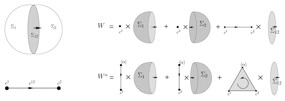
Figure 3: Top left: The manifold $M$ is divided into bulk regions $\Sigma_{1}$ and $\Sigma_{2}$ by the hypersurface $\Sigma_{12}$. For convenience $M$ is shown as a compact ball but we should emphasize that we are ignoring the boundary $\partial M$ at the moment. Bottom left: the corresponding dual cells $c^{1}$, $c^{2}$ and $c^{12}$ with orientation induced by the $\Sigma$’s. Top right: The secondary manifold of $M$ is $W=c^{1}\times\Sigma_{1}+c^{2}\times\Sigma_{2}+c^{12}\times\Sigma_{12}$. Bottom right: The smoothing manifold $W^{\alpha}=C(\alpha,c^{1})\times\Sigma_{1}+C(\alpha,c^{2})\times\Sigma_{2}+C(\alpha,c^{12})\times\Sigma_{12}$.

Requiring that this term vanish, there are two possibilities:
1) Continuous vielbein, discontinuous spin connection: If $E_{1}|_{\Sigma_{12}}=E_{2}|_{\Sigma_{12}}$ then $\omega_{\alpha}$ drops out of (33). Furthermore, since the vielbein is continous, the limiting value of the field $E_{\alpha}$ is well defined on $\Sigma_{12}$ and is given by:

$$\lim_{\alpha\to\infty}E_{\alpha}\big{|}_{\Sigma_{12}}=E_{1}\big{|}_{\Sigma_{12}}=E_{2}\big{|}_{\Sigma_{12}}\,.$$

The problematic term (33) vanishes in this case. So, by the smoothing theorem, in the limit that $\omega_{\alpha}$ becomes discontinuous, the action converges unambiguously to $I[E_{1},\!\omega_{1},\!E_{2},\!\omega_{2}]$, this being the sum of Einstein-Hilbert terms in the bulk plus a surface term:

$$I[E_{1},\!\omega_{1},\!E_{2},\!\omega_{2}] =\frac{1}{2}\int_{\Sigma_{1}}\!\epsilon(\Omega_{1}E_{1}E_{1})+\frac{1}{2}\int_{\Sigma_{2}}\!\epsilon(\Omega_{2}E_{2}E_{2})$$

$$\qquad+\frac{1}{2}\int_{\Sigma_{12}}\epsilon\big{(}(\omega_{2}-\omega_{1})E^{2}\big{)}\,.$$ (34)

In the absence of torsion, the continuity of the metric implies the continuity of the tangential components of the spin connection. In that case the surface term is the difference of the Gibbons-Hawking term on each side of $\Sigma_{12}$, as expected.

$$I[g_{1},g_{2}] =\int_{\Sigma_{1}}\!R_{1}\sqrt{-g_{1}}\,d^{4}x+\int_{\Sigma_{2}}\!R_{2}\sqrt{-g_{2}}\,d^{4}x$$

$$\qquad\mp 2\int_{\Sigma_{12}}(K_{2}-K_{1})\sqrt{\mp h}\,d^{3}x\,.$$ (35)

2) Discontinuous vielbein, continuous spin connection: If $\omega_{1}|_{\Sigma_{12}}=\omega_{2}|_{\Sigma_{12}}$ then $E_{\alpha}$ drops out of (33). The field $\omega_{\alpha}$ converges to a well defined value on $\Sigma_{12}$:

$$\lim_{\alpha\to\infty}\omega_{\alpha}\big{|}_{\Sigma_{12}}=\omega_{1}\big{|}_{\Sigma_{12}}=\omega_{2}\big{|}_{\Sigma_{12}}\,.$$

In this case also, the problematic term (33) vanishes, in spite of the fact that the limiting value of the vielbein $E_{\alpha}$ is undefined on $\Sigma_{12}$.

The secondary action has vanishing surface term on $\Sigma_{12}$:

$$I[E_{1},\!\omega_{1},\!E_{2},\!\omega_{2}] =\frac{1}{2}\int_{\Sigma_{1}}\!\epsilon(\Omega_{1}E_{1}E_{1})+\frac{1}{2}\int_{\Sigma_{2}}\!\epsilon(\Omega_{2}E_{2}E_{2})$$ (36)

The possibility of a well defined action for a discontinuous metric is quite remarkable. This can only happen if there is torsion. Let us introduce Gaussian normal co-ordinates $(\xi^{\mu},z)$ where and $\xi^{\mu}$ are tangential and $z$ is the normal co-ordinate, chosen so that the direction of increasing $z$ points from $\Sigma_{1}$ to $\Sigma_{2}$, with $\Sigma_{12}$ located at $z=0$. Then the allowed distributional parts of the torsion are:

$$T^{a}_{z\mu} =\left[(E_{2})^{a}_{\mu}-(E_{1})^{a}_{\mu}\right]\delta(z)+\left(\omega^{a}_{\ b\,z}[(E_{2})^{b}_{\mu}-(E_{1})^{b}_{\mu}]-\omega^{a}_{\ b\,\mu}[(E_{2})^{b}_{z}-(E_{1})^{b}_{z}]\right)H(z)+\cdots\,,$$

$$T^{a}_{\mu\nu} =\left(\omega^{a}_{\ b\,\mu}[(E_{2})^{b}_{\nu}-(E_{1})^{b}_{\nu}]-\omega^{a}_{\ b\,\nu}[(E_{2})^{b}_{\mu}-(E_{1})^{b}_{\mu}]\right)H(z)+\cdots\,.$$

These field configurations are very exotic- the metric is undefined at $\Sigma_{12}$. However, the metric is defined as the limit of smooth metrics and we have proven that it gives a well defined action. If one is performing a path integral for a theory with torsion, it seems that these field configurations should not be excluded.

In the case where both spin connection and vielbein are discontinuous, then the term (33) generally does not vanish. Indeed, making no assumptions about the limit of $E_{\alpha}$ and $\omega_{\alpha}$, it is undefined. Therefore situations 1) and 2) above exhaust the possibilities.

The method of the smoothing manifold has been used to find some new results for non-smooth geometry in Einstein-Cartan gravity. However, these results could certainly have been found using a less sophisticated formalism. Our approach really comes into its own when the action is nonlinear in the curvature. A good example is Lovelock gravity, to which we shall now turn our attention.

III.2 Lovelock-Cartan Gravity

Lovelock gravity in $D$ space-time dimensions is defined by a Lagrangian which is a sum of terms $\epsilon(\Omega\cdots\Omega E\cdots E)$. Let us just focus on a single term, polynomial of order $p$ in the curvature tensor.

$${\cal L}=\epsilon(\Omega^{p}E^{q})$$ (37)

with $2p+q=D$.

The secondary action is:

$${\cal K}=\epsilon([\delta\bar{\omega}+\bar{\Omega}]^{p}\bar{E}^{q}).$$ (38)

In order to apply the smoothing theorem, we will need the following result:

$$(d+\delta){\cal K}=q\sum_{s=-1}^{p-1}{\cal N}_{s}+q\sum_{s=0}^{p}{\cal M}_{s},$$ (39)

where ${\cal N}_{s}$ and ${\cal M}_{s}$ are differential forms of order $(s+1,D-s)$ in $(dt,dx)$ given by

$${\cal N}_{s} :=\frac{p!}{(s+1)!(p-s-1)!}\,\epsilon\left((\delta\bar{\omega})^{s+1}\bar{\Omega}^{p-s-1}\bar{T}\bar{E}^{q-1}\right)\,,$$

$${\cal M}_{s} :=\frac{p!}{s!(p-s)!}\,\epsilon\left((\delta\bar{\omega})^{s}\bar{\Omega}^{p-s}\delta\bar{E}\bar{E}^{q-1}\right)\,.$$ (40)

Let us analyse the behavior of the integral over the smoothing manifold. The integral is a sum of terms of the form:

$$q\int_{C(\alpha,c)}\int_{\Sigma}{\cal N}_{s}+{\cal M}_{s}\,,$$ (41)

where $\Sigma$ is a cell of codimension $s$. There are two generic ways to make the integral vanish:

Case 1) Continuous vielbein, zero torsion, discontinuous spin connection: The cell $\Sigma$ is the intersection of a collection of $n$ bulk cells $\{\Sigma_{i}|i\in(1,\dots,n)\}$. Suppose that the intrinsic veilbein $E\big{|}_{\Sigma}$ on $\Sigma$ is well defined i.e. $E_{i}\big{|}_{\Sigma}=E\big{|}_{\Sigma}\ \forall\ i\in(1,\dots n)$. The pullback of $E_{\alpha}$ therefore converges to a well defined value $\lim_{\alpha\to\infty}E_{\alpha}\big{|}_{\Sigma}=E\big{|}_{\Sigma}$. This implies that the contribution of ${\cal M}_{s}$, being proportional to $\delta\bar{E}$, vanishes.

Now we observe that $\bar{T}=\sum_{i}t^{i}T_{i}+\sum_{i,j}t^{i}t^{j}\omega_{i}(E_{j}-E_{i})$. The first term vanishes by zero torsion and the second by continuity of the vielbein. Therefore the contribution of ${\cal N}_{s}$, being always proportional to $\bar{T}$, vanishes.

Case 2) Continuous spin connection, discontinuous vielbein: In this case the pullback of $\delta\bar{\omega}$ vaishes. The only terms which survive are ${\cal N}_{-1}$ and ${\cal M}_{1}$. ${\cal N}_{-1}$ is a form of order $(0,D+1)$ so its pull-back identically vanishes. ${\cal M}_{1}$ is of order $(1,D)$ so it is to be integrated over $C(\alpha,c^{i})\times\Sigma_{i}$ where $\Sigma_{i}$ is a bulk cell. But, by construction $E_{\alpha}$ coincides with $E_{i}$ in the bulk so the pull back of $\delta\bar{E}$ onto $C(\alpha,c^{i})$, and thus also ${\cal M}_{1}$, vanishes.

The above two cases are the generic ways to satisfy the smoothing theorem. There may also be some special cases depending on the dimensionality of the cells at which the discontinuity occurs and on which Lovelock terms are present in the action.

Note that our method applies to situations where the spin connection is at worst $C^{1-}$ so solutions with solid angle defects of higher codimension Charmousis:2005ey Zegers-08 fall outside of our analysis.

IV Homotopy and ‘renormalization’

Up to this point we have presented some answers to questions posed at the beginning of our work, but various issues remain still open. Is the secondary manifold $W$ in any sense unique and what does it mean if it is not? What happens if the manifold $M$ has a boundary? What is the relation between the smoothability of the action and that of the equations of motion? In this and the next section we discuss these matters and their implications.

IV.1 The dual complex as a geometric complex

Before going to analyze these issues we would like to discuss a bit our requirement that the dual complex be homoemorphic to a geometric simplicial complex. In particular to discuss certain reasonable configurations which have to be excluded from a general formulation because they bring bad company along with them. Being half-justifiably sacrificed, they deserve now an honorary mention.

Consider the configurations whose cross-sections are shown in the figure 4: due to their similarity to Feynman graphs we call them self-energy and tadpole graphs (they are given by the continuous lines). These are reasonable intersections because, i) locally, they look everywhere just fine and our considerations start from local features, ii) there is a way to get them from intersections with a geometric dual complex (as shown by the dashed lines and we explain below). This latter fact is also a difficulty.

Self-energy is the better character of the two. It has this feature: the boundary map $\partial$ acting on the $\Sigma$ cell complex gives zero only acting at the highest co-dimension cells (one may say its kernel is ‘trivial’). This is a good postulate for the cell complex but excludes the tadpole, which as said already is fairly reasonable. Put differently, an intersection like the tadpole involves cells that have been identified along their boundary to some extent.

Practically the problem is that if we apply the rules (12) and (15) the thing works but we obtain dual cell complexes that look strange. We want to express the Lagrangian terms of each $\Sigma$ cell as integrals over plain Euclidean simplices. Perhaps not surprisingly the problem can be fixed: One way to look at it is that there are not enough bulk regions in these configurations. So we may imagine, or start with and then set to zero, new discontinuities (dashed lines) subdividing the existing bulk regions and their boundaries. Then, as shown in figure 4, the dual complex is a geometric complex. Integrating the secondary Lagrangian over it, certain cells will simply not contribute in the action as the fields are continuous across the respective $\Sigma$ cells.

Figure 4: Upper left: ‘Self-energy’, Upper right: ‘Tadpole’. Bottom: The respective geometric dual complexes.

So every time we have mentioned ‘bulk cells’ above, it could mean bulk cells obtained by subdividing the initial bulk cells of a configuration in a way to end up with geometric dual space. But if we want to make all the distinction of what we can and cannot describe at the level of the cell complexes, here lies the difficulty. Imagine a single half-infinite hypersurface in spacetime i.e. the connection is discontinuous only across. (Presumably this is like a tadpole with a collapsed ‘circle’.) We can now imagine two other (‘dashed’) half-infinite hypersurfaces forming a 3-way intersection with it, a perfectly legitimate configuration. For many Lagrangians (e.g. Lovelock gravities) we will find no term for the co-dimension 2 cell this way. But we actually have a localized holonomy here and there must certainly be such a term. So at this point we think we have honored the victims enough. Empirically they are of course acceptable. We will not try to refine further the cell complex postulates in this work.

IV.2 The homology class of the secondary manifold

Let us now turn to our questions at beginning of this section. First of all, if for some configuration we can manufacture a manifold $W$ and prove smoothability, criterion II.13, then we definitely have a well-defined action for the distributional fields, the secondary action $\int_{W}{\cal K}$. We may now explore the following: The secondary manifold has been defined essentially through the boundary relations (15). They are chosen so that if $M$ has no boundary then $\partial W=\varnothing$; that is all they contain. Such a condition does not define the secondary manifold uniquely; the transformation $W\to W+\partial Y$ preserves the condition. Therefore $W+\partial Y$ can also be picked as the secondary manifold, for any $Y$ such that $\partial Y$ and $\partial\partial Y=\varnothing$ make sense. That is any given $W$ is a representative of a homology class defined as the equivalence class $W\sim W+\partial Y$. Fix a cell complex $\{\Sigma_{A}\}$. Recalling the definition II.6, the general$D$-dimensional chain of such a cell complex reads

$$Y=\sum_{A}d^{A}\times\Sigma_{A}\,.$$ (42)

Each $d^{A}$ is an arbitrary cell of dimension $|A|+1$ homeomorphic to chains of that dimension on a simplex, $S$, of very large dimension. Recall that $|A|$ is the co-dimension of $\Sigma_{A}$. [The set of chains of $S$ is the large cell complex which ‘accommodates’ all our cells and complexes.]

Then

$$W+\partial Y=\sum_{A}\hat{c}^{A}\times\Sigma_{A}\,,$$ (43)

where

$$\hat{c}^{A}=c^{A}+\partial d^{A}+\sum_{B}(-1)^{|B|+1}\,\epsilon(A,B)\,d^{B}\,.$$ (44)

Using $\sum_{C}\epsilon(A,C)\epsilon(C,B)=0$ one finds that the cells $\hat{c}^{A}$ do indeed satisfy the same relations as the cells $c^{A}$:

$$\partial\hat{c}^{A}=\sum_{B}(-1)^{|B|+1}\,\epsilon(A,B)\,\hat{c}^{B}\,,$$ (45)

i.e. the incidence numbers $\epsilon(A,B)$ appearing here and in (15) are the same. Thus we have: the cells $c^{A}$ and $\hat{c}^{A}$ related by (44) are equivalent choices for dual cells. That is, if $\{\Sigma_{A}\}$ is a given cell complex, then $\{c^{A}\}$ and $\{\hat{c}^{A}\}$ are equivalent choices for the cell complex dual to $\{\Sigma_{A}\}$. Thus we arrive at the following

Definition IV.1.

The set of all homomorphic cell complexes, i.e. complexes with the same incidence numbers, will be called a cell structure. A given cell complex is a representative of the cell structure. [When no confusion arises we denote the structure by one representative.]

Using this terminology we may say that a cell complex $\{\Sigma_{A}\}$ defines a dual cell structure, not a single dual cell complex. It turns out that that the cell structure can be viewed also as a homotopy class. From (45) we have that a linear combination of the cells $c^{A}$ becomes a linear combination of $\hat{c}^{A}$ if induced by the same linear combination of $d^{A}$. That is, an operator $\mathbf{P}$ defined by $d^{A}=\mathbf{P}c^{A}$ is a linear operator acting on cells viewed as chains. Then (44) tells us that

$$\hat{c}^{A}=c^{A}+\partial\mathbf{P}c^{A}+\mathbf{P}\partial c^{A}\,.$$ (46)

In topology chains $c^{A}$ and $\hat{c}^{A}$ related this way are said to be chain-homotopic and the linear map $\mathbf{P}$ a chain-homotopy Hatcher . Thus $\mathbf{P}$ moves the dual cells around in the dual cell structure. Now any two elements in the structure are not obviously homotopic. On the other hand their defining relation (15) is linear. That is the structure is a linear space. There is always a linear map $\rho$ between any two cell complexes. Using linearity it is straightforward to show via (15) that $\partial\,\rho=\rho\,\partial$. That is, $\rho$ is a chain-map. Thus any two elements in the structure are related by a chain map. Chain-maps fall into homotopy classes. Let $\mathbf{P}$ be a linear map from cells of dimension $|A|$ to ones of dimension $|A|+1$. Then $\partial\mathbf{P}+\mathbf{P}\partial$ is linear and commutes with $\partial$ (by $\partial\partial=0$). Thus $\rho$ falls into some equivalence class $\{\rho\thicksim\rho+\partial\mathbf{P}+\mathbf{P}\partial\}$. That is any chain-map belongs into an equivalence class of chain-homotopic maps. In other words, the structure is in general a disjoint union of chain-homotopic classes of cells.

There is a slightly different kind of homotopy operator which can be naturally put on the same footing as $\mathbf{P}$. It is the cone operator whose action is defined by (16). A cell complex which contains only a vertex, $\{\langle*\rangle\}$, satisfies any given boundary rules (15), by $\partial\langle*\rangle=0$. That is $\{\langle*\rangle\}$ belongs to any given dual cell structure. The cone operator $C(*,\cdot)$ serves as a homotopy between $*$ and other cell complexes. Given a cell $c^{A}$ and a vertex $*$, is it always possible to form the cone $C(*,c^{A})$? The answer is yes: all our complexes essentially reside in the infinite dimensional geometric simplex $S$. This is a contractible space therefore homotopy, and homology as well, are trivial. This reflects the properties we require at the level of fields: we want to approximate in a continuous manner piece-wise smooth configurations of $\{\Psi_{i}\}$ by single smooth fields $\Psi_{\alpha}$.

Corollary IV.2.

There is a single chain-homotopy class in the dual cell structure. I.e. the structure is a homotopy class itself.

We shall use this fact repeatedly in what follows. Define now the action of $\mathbf{P}$ on chains of the product complex $\{c\times\Sigma\}$, or more generally on a cell complex of $\Sigma$ cells with dual-cell-valued coefficients, as a linear operator acting by $\mathbf{P}(c^{A}\times\Sigma_{B}):=(\mathbf{P}c^{A})\times\Sigma_{B}$. By this definition one finds that

$$(\partial\mathbf{P}+\mathbf{P}\partial)(c^{A}\times\Sigma_{B})=((\partial\mathbf{P}+\mathbf{P}\partial)c^{A})\times\Sigma_{B}\,.$$ (47)

That is $\mathbf{P}$ naturally extends to a homotopy of chains on a product complex, thus we will not use a different symbol for that extension. Then we have that the chain $\hat{W}\equiv\sum_{A}\hat{c}^{A}\times\Sigma_{A}$ of (43) can be written as

$$\hat{W}=W+\partial(\mathbf{P}W)+\mathbf{P}(\partial W)\,.$$ (48)

Recall that for $\partial M=\varnothing$ we have $\partial W=\varnothing$ and therefore: $\mathbf{P}$ moves the secondary manifold around in a homology class.

Definition IV.3 (Secondary manifold and its class).

Let $\{\Sigma_{A}\}$ be a cell complex whose union is a manifold $M$ without boundary. The secondary manifold is a representative of a homology class (the secondary manifold class $\mathcal{W}_{\Sigma}$) of chains in the $\Sigma$ cell complex with cell-valued coefficients in the dual cell structure.

That is, the secondary manifold is one element of a homology class which is itself a homotopy invariant (with respect to the dual space). By the previous corollary the dual cell structure is unique. That is the class $\mathcal{W}_{\Sigma}$ is unique. This is our answer to the question of uniqueness of the secondary manifold. Now this is a general mathematical result. A question which arises is:

Question IV.4.

What are all the different representatives of the secondary manifold class $\mathcal{W}_{\Sigma}$?

We take on answering that question after we digress to deal with the case of $M$ with boundary.

IV.3 Manifolds with boundary

Let now $M=\bigcup_{A}\Sigma_{A}$ possess a boundary. Then some of the cells will have a part of their boundary contained in $\partial M$. Therefore we will generalize the boundary rule on cells as

$$\partial\Sigma_{B}=\sum_{A}\epsilon(A,B)\Sigma_{A}+X_{B}\,,$$ (49)

where $X_{B}=\partial\Sigma_{B}\cap\partial M$. Of course for some of the values of the label these cells are empty.

$\partial\partial=0$ holds if and only if $\sum_{A}\epsilon(A,B)X_{A}+\partial X_{B}=0$. This means that the boundary cells form a cell complex with incidence numbers $-\epsilon(A,B)$. Thinking intrinsically of the boundary $\partial M$ as a separate manifold, the cells dual to $\{X_{A}\}$ obey

$$\partial c_{\|}^{A}=\sum_{B}(-1)^{|B|}\,\epsilon(A,B)\,c_{\|}^{B}\,.$$ (50)

($|A|$ correctly gives the dimension of $c^{A}_{\|}$ and the co-dimension of $\Sigma_{A}$.) Thus we deal with the boundary dual cell structure.

The relation (50) is satisfied also by the cells $(-1)^{|A|}\,c^{A}$. That is, these cells can be representatives of the boundary dual cell structure, one may say ‘extrinsic’ ones. If it is unique, which we assume, then the structures $\{c^{A}_{\|}\}$ and $\{(-1)^{|A|}\,c^{A}\}$ coincide. Thus their cells are homotopic. In other words there exists an operator $\mathbf{P}_{\|}$ such that $\partial\mathbf{P}_{\|}c^{A}=(-1)^{|A|}\,c_{\|}^{A}-c^{A}-\mathbf{P}_{\|}\partial c^{A}$.

The cells $\mathbf{P}_{\|}((-1)^{|A|}c^{A})$ are interpolations between the ‘intrinsic’ and ‘extrinsic’ dual cells for $X_{A}$ as cells in $\partial M$. They also have the right dimension and boundary rule for dual cells of $X_{A}$ as cells in $M$.

On the direct sum of cell and boundary cell complexes (with cell-valued coefficients) define the $D$-chain

$$W:=\sum_{A}\left\{c^{A}\times\Sigma_{A}+(-1)^{|A|}\mathbf{P}_{\|}c^{A}\times X_{A}\right\}\,.$$ (51)

It will be useful to note the usual boundary rule (15) of the dual cells reads also $(-1)^{|A|}\partial c^{A}=\sum_{B}\epsilon(A,B)\,c^{B}$. We may use this to show that

$$\partial W=\sum_{A}c_{\|}^{A}\times X_{A}\,.$$ (52)

As $\bigcup_{A}X_{A}=\partial M$ the manifold on the r.h.s. is nothing but a secondary manifold associated with the cell structure in $\partial M$.

The reason why the secondary manifold is defined by the chain $W$ above, is probably better understood by considering the action of the cone-product which served in providing the right formulas to state the ‘smoothing theorem’ II.13 and also discussed in the previous section. The cone-product is a chain-homotopy $\mathbf{P}=C(*,\cdot)$ between any cell and a vertex $\langle*\rangle$. By its very properties and the previous result we find:

$$\partial C(*,W)=W-\left\{\sum_{i}\langle*\rangle\times\Sigma_{i}+\sum_{A}C(*,c^{A}_{\|})\times X_{A}\right\}\,.$$ (53)

$\sum_{i}\Sigma_{i}=M$. The single vertex $\langle*\rangle$ represents smooth fields over $M$. In the presence of a boundary $\partial M$ the action is defined by integrating the secondary Lagrangian over the manifold in the brackets. That, for example, reproduces the York (or Gibbons-Hawking) action of general relativity. Thus $C(*,W)$ is again the smoothing manifold, generalizing the discussion of section II.3 in the presence of a boundary.

Consider now the action of an arbitrary homotopy on the chains (51). This involves a product of homotopy operators. It will be convenient at this point to get more geometric. If a chain $c$ is homotopic to a chain $\hat{c}$ via a homotopy $\mathbf{P}$, relation (46), we may define their prism product which is the cell $P(\hat{c},c):=\mathbf{P}c$. From (46) we have that $\partial P(\hat{c},c)=\hat{c}-c-P(\partial\hat{c},\partial c)$. Geometrically this makes sense as being the boundary of the prism $P(\hat{c},c)$ with $\hat{c}$ and $c$ as ‘top’ and ’bottom’ sides.

Let us consider four homotopic cell complexes, $(-1)^{|A|}c^{A}_{\|}$, $(-1)^{|A|}\hat{c}^{A}_{\|}$, $c^{A}$ and $\hat{c}^{A}$, all representatives of the single cell structure. In particular let $c$ be a complex and $(-1)^{|c|}c_{\|}$ be a boundary complex which is homotopic to it via a homotopy $\mathbf{P}_{\|}$. Let $\mathbf{P}$ be a homotopy which sends $c$ to $\hat{c}$ and $c_{\|}$ to $\hat{c}_{\|}$. There will also be a homotopy $\mathbf{\hat{P}}_{\|}$ between $\hat{c}$ and $(-1)^{|c|}\hat{c}_{\|}$. Now the cells $P(\hat{c}^{A},c^{A})$ and $P((-1)^{|A|}\hat{c}^{A}_{\|},(-1)^{|A|}c^{A}_{\|})=(-1)^{|A|}\,P(\hat{c}^{A}_{\|},c^{A}_{\|})$ are also homotopic. Thus there exists a homotopy $\mathbf{\overline{P}}$ between them, whose restriction acting on $c$’s and $c_{\|}$’s is $\mathbf{P}$. Similarly there exists a $\mathbf{\overline{P}}_{\|}$ sending the $c$’s to the $c_{\|}$’s. The maps are depicted schematically for 0-cells in figure 5.

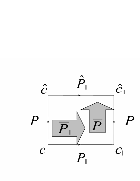
Figure 5: Schematic representation of the action of operators $\mathbf{\overline{P}}$ and $\mathbf{\overline{P}}_{\|}$.

This diagram shows that the relation $\mathbf{\overline{P}}_{\|}\mathbf{P}=\mathbf{\overline{P}}\mathbf{P}_{\|}$, of composition of maps, should hold. This relation is useful in detailed calculations.

Consider now a homotopy of the $D$-chain $W$ in (51), that is, as we have defined it, a homotopy of its dual cell-valued coefficients. Let that be effected by an operator $\mathbf{\overline{P}}$ as defined above. Then we have that

$$\partial\mathbf{\overline{P}}W=\hat{W}-W-\mathbf{\overline{P}}(\partial W)\,.$$ (54)

Formula (52) tells that the last term on r.h.s. equals to

$$-\sum_{A}(\mathbf{\overline{P}}c_{\|}^{A})\times X_{A}\,.$$ (55)

that is the dual cell coefficients are prisms $P(\hat{c}_{\|}^{A},c_{\|}^{A})$.

Now require that the boundary complexes be one and the same: $\hat{c}_{\|}^{A}=c_{\|}^{A}$. Then their prism $P(\hat{c}_{\|}^{A},c_{\|}^{A})=\varnothing$. Thus we have:

Theorem IV.5.

Let $\{\Sigma_{A}\}$ be a cell complex with $M=\bigcup_{A}\Sigma_{A}$ a manifold with a boundary $\partial M=\bigcup_{A}X_{A}$. Fix a dual cell complex $c_{\|}$ for the boundary cells $X_{A}$. Define $D$-chains on the direct sum of the $\Sigma$ cell complex (with dual cell-valued coefficients $c$) and $X$ cell complex (with coefficients $P(c_{\|},(-1)^{|c|}c)=(-1)^{|c|}\mathbf{P}_{\|}c$). Their homology class is a homotopy invariant, in the way of the coefficients, under all homotopies that leave $c_{\|}$ unchanged.

In the spirit of the definition IV.3, we define here in the same way but more generally, the secondary manifold class $\mathcal{W}$ to be this homology class. The secondary manifold is any representative of this class. In the next section we give an interpretation of those different forms of the secondary manifold.

We close the section by discussing an important use of the results obtained here, and simultaneously take care of a difficulty which we face when considering real examples.

In order to formulate and prove the well defined smooth limit of non-smooth configurations, we integrate Lagrangians over the whole of $M$ and $W$ as a necessary ingredient in the derivations. That is not satisfying because (i) for $M$ with or without boundary, it brings in the asymptotic behavior of the fields which might be such that the action diverges and (ii) it makes completely local questions like the smoothability of a local discontinuity dependent on what happens on the whole of $M$.

Being able to treat a manifold with boundary it means that we can integrate Lagrangians over arbitrary regions $R\subset M$ with smooth boundary $\partial R$ such that no singularities unrelated to the discontinuities themselves are involved. That of course makes our considerations as local as we want.

IV.4 ‘Renormalization’

In simple examples the non-uniqueness of $W$ arises in the form of multiple but apparently equivalent choices for the dual cells as chains of simplices.

Such an example is shown at the top of figure 6a, a cross section of a 4-way intersection of hypersurfaces. Its dual cell is shown at the bottom (in solid line). That cell can be expressed as a chain of simplices in at least two ways: one may divide it along any of its diagonals. In the figure we draw one of these two cases. The diagonal is not dual to a hypersurface and it is shown by a dashed line.

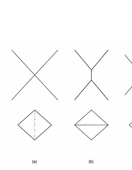
Figure 6:

These two abstract chains can be thought of as chains residing in the geometric cell complexes shown at the bottom of figures 6b and 6c. In each case they are the sum of the two 2-simplices in the cell complex. Any one of the two chains can be used in writing down explicitly the secondary manifold.

These chains are homotopic. One constructs a prism ‘interpolating’ between the corresponding abstract cells. In our case this is a singular parallelepiped (that is, some general deformation of the Euclidean one). A prism is the value of a homotopy map evaluated at a cell. So there is a homotopy between the cells. Each cell is a different chain of simplices. I.e. it is triangulated. We may further subdivide each cell to reach a common triangulation between them. This is shown in figure 7.

Figure 7:

So we can ‘match’ their simplices. It is then a mere technicality to explicitly construct a chain-homotopy between them, which is standard in the literature Hatcher . Thus one proves the homotopy of cells as chains. One can construct the simplices we started with from the smaller simplices of the finer triangulation.

Thus the difference in the choices we have when writing down the secondary manifold in the 4-way intersection is about homotopy of the dual chains. As we saw in the previous sections this means that the two secondary manifolds differ by a boundary. We also saw that starting from the latter point it is natural to think in terms of the whole homotopy class of the dual chains, that is, the dual cell structure .

Up to this point the ‘Compton scattering’ configurations in the figures 6b and 6c have been neglected. They are there because they turned out to have dual cell complexes homotopic to that of the 4-way intersection(i.e. also to each other). The picture is suggestive as to why this is so: These intersection can be deformed, by continuously ‘collapsing’ the intermediate hypersurface, to become the 4-way intersection. We can also imagine the reverse course of deformation, or them deforming to each other. (I.e. they are homotopic themselves.) The more complicated ‘Compton’ configurations, seen from a ‘distance’, they will look just like the 4-way intersection. The other way around, from a distance we might view the latter as two connected more elementary (simplicial) intersections with vanishing separation.

This suggests something: It might be the case that the many different homotopic dual cell complexes possible for a given cell complex $\{\Sigma\}$ are remnants of the many cell complexes that, when viewed from a distance, look like $\{\Sigma\}$. Or, put differently, those that become $\{\Sigma\}$ in the limit of appropriate deformations.

In the rest of this section we shall show that the general effect of such limits is to move the secondary manifold around within its class $\mathcal{W}_{\Sigma}$. This will provide the interpretation we will looking for in question IV.4. Before doing so we describe another kind of characteristic example.

The configurations in figure 6 can be described as ‘tree level’ deformations of each other. Instead, consider the configuration at the top of the figure 8a. Collapsing the central loop to zero size the configuration deforms to the 3-way intersection on the right. Its dual cell complex (in solid line) is homotopic to the cell complex of the loop configuration: subdividing it up as the dashed lines show in figure 8b we can ‘match’ the smaller simplices.

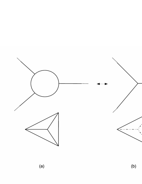
Figure 8:

These deformations can be described as ‘loop level’ ones and introduce a new feature: the subdivision of the dual cell complex introduces a new vertex. On the cell complex (configurations) side and in the reverse course, a bulk region is collapsed. Seen from a distance, a loop with vanishing size could be taken for the 3-way intersection. Thus we may consider a limit that does that. The two dual complexes being homotopic, we will end up with a secondary manifold which differs only by a boundary from the old one, i.e. we deal with two elements of the same secondary manifold class.

At this point, we might wonder whether such ‘nearby’ configurations translate necessarily to nearby descriptions at the level of fields satisfying their equations. This matter will be become rather straightforward after we have established what happens at the level of the secondary manifold, to which we proceed.

Let $\{\bar{\Sigma}_{I}\}$ be a cell complex such that $\bigcup_{I}\bar{\Sigma}=M$ point set-wise. Let a continuous map $\mu:M\to M$ which shifts point in a continuous manner such that now $M=\bigcup_{A}\Sigma_{A}$ for a cell complex $\{\Sigma_{A}\}$. I.e. $\mu$ is a continuous deformation of the net of cells $\bar{\Sigma}_{I}$. Some of them will be driven to extinction, at least as cells of co-dimension $|I|$.

In general $\mu$ will act as a deformation retraction for collections of cells $\bar{\Sigma}_{I}$, of highest co-dimension $|A|$, for some $A$, to a cell $\Sigma_{A}$. By construction, this happens for all $A$. These collections of cells form sub-complexes of $\{\bar{\Sigma}_{I}\}$ which we denote by $\{\bar{\Sigma}\}_{\!A}$. We defined them to be the largest ones with the required property. Thus they cover the initial cell complex: $\bigcup_{A}\{\bar{\Sigma}\}_{\!A}=\{\bar{\Sigma}_{I}\}$ as sets of cells. Note that $\{\bar{\Sigma}\}_{\!A}$ are in one-to-one correspondence with $\Sigma_{A}$.

In each complex $\{\bar{\Sigma}\}_{\!A}$ we form chains $\bar{\Sigma}_{A}:=\sum_{I}\bar{\Sigma}_{I}\,\mu(I,A)$, of co-dimension equal to $|A|$ i.e. built out of the highest co-dimension cells in the complex. That is, the numbers $\mu(I,A)=0$ unless $|I|=|A|$. Moreover, we require them to satisfy

$$\sum_{I}\bar{\epsilon}(J,I)\,\mu(I,A)=\sum_{B}\mu(J,B)\,\epsilon(B,A)\,,$$ (56)

where $\epsilon$ and $\bar{\epsilon}$ are the incidence number matrices of the cell complexes $\{\Sigma_{A}\}$ and $\{\bar{\Sigma}_{I}\}$ respectively. In matrix notation (56) reads $\bar{\epsilon}\mu=\mu\epsilon$.

The idea is of course that in each complex $\{\bar{\Sigma}\}_{\!A}$ only the cells appearing in $\bar{\Sigma}_{A}$ will not extinct under $\mu$, or ‘collapse’ as we shall prefer to say. They will simply be superposed to form $\Sigma_{A}$. By $\mu(I,A)$ we fiddle the orientations of this superposition.

We shall call such a complex $\{\bar{\Sigma}_{I}\}$ a renormalization of the cell complex $\{\Sigma_{A}\}$.

By definition chains over a cell complex form a vector space. We define a linear map from $\{\bar{\Sigma}_{I}\}$ to $\{\Sigma_{A}\}$, meaning between the respective spaces of chains, denoted also by $\mu$, which encodes the effect of the retraction $\mu$ on points but also assumes linearity acting on cells. Specifically we define it such that $\mu(\bar{\Sigma}_{A})=\Sigma_{A}$, though this just a matter of convenience. More importantly, for cells $\bar{\Sigma}_{I}$ that extinct under the retraction, at least as cells of the specific co-dimension, we set $\mu(\bar{\Sigma}_{I})=\varnothing$.

Corollary IV.6.

The linear map $\mu:\{\bar{\Sigma}_{I}\}\to\{\Sigma_{A}\}$ which encodes the effects of the retraction $\mu$ is a chain map i.e. $\partial\,\mu=\mu\,\partial$.

Proof. Let a cell $\{\bar{\Sigma}_{I}\}$. Under ‘collapse’ three things may happen: i) The cell itself collapses, ii) a cell $\bar{\Sigma}_{J}$ in its boundary $\partial\bar{\Sigma}_{I}=\sum_{J}\,\bar{\Sigma}_{J}\,\bar{\epsilon}(J,I)$ collapses, iii) i) and ii) do not apply even inductively.

In iii) $\mu$ acts as the identity so it definitely commutes with $\partial$. In i) $\partial\mu(\bar{\Sigma}_{I})=\partial\varnothing=\varnothing$. Also $\mu(\partial\bar{\Sigma}_{I})=\sum_{J}\mu(\bar{\Sigma}_{J})\,\bar{\epsilon}(J,I)$. $\bar{\Sigma}_{I}$ collapses thus $\bar{\Sigma}_{J}$ either collapse themselves, or retract to a single highest co-dimension cell. In the latter case $\mu(\bar{\Sigma}_{J})$ will cancel each other due to opposite orientations. In both cases $\mu(\partial\bar{\Sigma}_{I})=\varnothing=\partial\mu(\bar{\Sigma}_{I})$.

In ii) $\mu(\partial\bar{\Sigma}_{I})=\sum_{J^{\prime}}\,\mu(\bar{\Sigma}_{J^{\prime}})\,\bar{\epsilon}(J^{\prime},I)$, where $J^{\prime}$ sum over all relevant $J$ except those that $\mu(\bar{\Sigma}_{J})=\varnothing$. On the other hand the boundary $\partial$ of $\mu(\bar{\Sigma}_{I})$ includes those cells of one co-dimension higher except those that $\mu(\bar{\Sigma}_{J})=\varnothing$. That is $\partial\mu(\bar{\Sigma}_{I})=\sum_{J^{\prime}}\,\mu(\bar{\Sigma}_{J^{\prime}})\,\bar{\epsilon}(J^{\prime},I)=\mu(\partial\bar{\Sigma}_{I})$. Thus in all cases we have that $\partial\,\mu=\mu\,\partial$. $\square$

The coefficients $\mu(I,A)$ in the definitions of the chains $\bar{\Sigma}_{A}$ are required to satisfy the relations (56) so that the chains satisfy $\partial\bar{\Sigma}_{A}=\sum_{B}\,\bar{\Sigma}_{B}\,\epsilon(B,A)$. Then corollary IV.6 allows us to deduce that $\partial\mu(\bar{\Sigma}_{A})=\sum_{B}\,\mu(\bar{\Sigma}_{B})\,\epsilon(B,A)$. Thus $\mu(\bar{\Sigma}_{A})=\Sigma_{A}$ is a consistent requirement on $\mu$. These two requirements are adequate conditions to translate the correspondence between $\{\bar{\Sigma}\}_{\!A}$ and $\Sigma_{A}$ from the level of sets to the level of cell complexes.

Let cells $c^{A}$ and $\bar{c}^{I}$ dual to the cells $\Sigma_{A}$ and $\bar{\Sigma}_{I}$ respectively. Let also cells $\bar{c}^{A}$ dual to the chains $\bar{\Sigma}_{A}$. The relations (56) allows us to show that the chains $\sum_{A}\mu(I,A)\bar{c}^{A}$ have the same boundary rules as the cells $\bar{c}^{I}$. According to our assumptions the dual structures are unique. That is, those two cell complexes must be homotopic. The same apply between the cell complexes $\bar{c}^{A}$ and $c^{A}$. Thus a $\bar{c}^{I}$ should be equal to $\sum_{A}\mu(I,A)c^{A}$ up to homotopies of the cells.

Note also the following. In matrix notation (56) reads $\bar{\epsilon}\mu=\mu\epsilon$. Similarly (13) may be written $\epsilon\epsilon=0$ and $\bar{\epsilon}\bar{\epsilon}=0$. Thus any given matrix $\mu$ satisfying (56) is one member of an equivalence class of such matrices: $\{\mu\thicksim\tilde{\mu}=\mu+\bar{\epsilon}\Pi+\Pi\epsilon\}$ where $\Pi(I,A)$ is any matrix of the right dimension. That is, any chain $\sum_{A}\tilde{\mu}(I,A)\bar{c}^{A}$ has the same boundary rules as the cells $\bar{c}^{I}$. One may verify that directly.

Thus in general we may write

$$\bar{c}^{I}= \sum_{A}\,\Big{\{}\tilde{\mu}(I,A)\big{(}c^{A}+\partial d^{A}+\sum_{B}(-1)^{|B|+1}\epsilon(A,B)d^{B}\big{)}\Big{\}}$$

$$-\partial\bar{d}^{I}-\sum_{J}\,(-1)^{|J|+1}\bar{\epsilon}(I,J)\bar{d}^{J}\,.$$ (57)

$d^{A}$ is a cell of dimension $|A|+1$. It can be thought of as the image of $c^{A}$ under a chain-homotopy, $d^{A}=\mathbf{P}c^{A}$. Similarly for $\bar{d}^{I}$. Note that $\bar{d}^{I}$ are general cells homeomorphic to chains of dimension $|A|+1$ of the geometric simplex $S$, no different than $d^{A}$.

Now, are all cells of the complex $\{\bar{c}^{I}\}$ represented this way?

The answer is no. In detail what happens is: For cells of the complex $\{\bar{\Sigma}_{I}\}$ which extinct under collapsing to $\{\Sigma_{A}\}$, there will not be a way to manufacture their duals from the dual cells of $\{\Sigma_{A}\}$. We have two cases. First, those $\bar{c}^{I}$ which are not dual to collapsed bulk regions i.e. they are not vertices. They can be effected by prisms $\bar{d}^{I}$ which are cones. Secondly, those vertices which are dual to collapsed bulk regions. Let us denote them by $\bar{\Sigma}_{\bar{i}}$ and the dual vertices by $\langle\bar{i}\rangle$.

Having picked a dual complex $\bar{c}^{I}$ to the complex $\bar{\Sigma}_{I}$ we can write down the secondary manifold: $\bar{W}=\sum_{I}\bar{c}^{I}\times\bar{\Sigma}_{I}$. Using (IV.4) and bearing in mind the previous remarks one finds:

$$\bar{W}=\sum_{A}c^{A}\times\bar{\Sigma}_{A}+\partial\bar{Y}+\sum_{\bar{i}}\langle\bar{i}\rangle\times\bar{\Sigma}_{\bar{i}}\,,$$ (58)

where the manifold $\bar{Y}$ is explicitly given by

$$\bar{Y}=\sum_{I}f^{I}\times\bar{\Sigma}_{I}\,,$$ (59)

$$f^{I}=\sum_{B}\big{\{}(-1)^{|B|}\,\Pi(I,B)\,c^{B}+\tilde{\mu}(I,B)\,d^{B}\big{\}}+\bar{d}^{I}\,.$$

To derive this result we use the fact that $\epsilon(A,B)=0$ unless $|A|=|B|+1$, which allows us to write the boundary rules in the form $\sum_{B}\epsilon(A,B)c^{B}=(-1)^{|A|}\partial c^{A}$, and the properties of the coefficients $\mu(I,A)$.

Define a natural extension of $\mu$ acting on chains of $\{\bar{\Sigma}_{I}\}$ from number-valued to dual cell-valued coefficients to be the linear map, denoted again by $\mu$, defined by

$$\mu(\bar{c}^{I}\times\bar{\Sigma}_{J}):=\bar{c}^{I}\times\mu(\bar{\Sigma}_{J})\,.$$ (60)

One may verify that this is a chain map: $\partial\,\mu=\mu\,\partial$.

$\bar{\Sigma}_{\bar{i}}$ are the collapsed bulk regions. That is $\mu(\bar{\Sigma}_{\bar{i}})=\varnothing$. We have

$$\mu(\bar{W})=\sum_{A}c^{A}\times\Sigma_{A}+\partial Y\,,$$ (61)

where we defined $Y=\mu(\bar{Y})$. $Y$ is a chain of dimension $D+1$ over the complex $\{\Sigma_{A}\}$ with cell-valued coefficients. The chain $\sum_{A}c^{A}\times\Sigma_{A}$ is a secondary manifold for this complex.

In more general terms our results can be stated as follows.

Theorem IV.7.

Let $\{\Sigma_{A}\}$ be a cell complex with $M=\bigcup_{A}\Sigma_{A}$ a manifold without boundary, and $\mathcal{W}_{\Sigma}$ its secondary manifold class. Let a renormalization $\{\bar{\Sigma}_{I}\}$ of $\{\Sigma_{A}\}$ with a secondary manifold class ${\mathcal{W}}_{\bar{\Sigma}}$. Then $\mu(\mathcal{W}_{\bar{\Sigma}})=\mathcal{W}_{\Sigma}$.

The result (61) provides an answer to the question IV.4. We have a general process producing arbitrary cobordisms $Y$ between elements of the secondary manifold class $\mathcal{W}$. Thus we may interpret the different secondary manifolds in $\mathcal{W}$ as different collapsed renormalizations of any given secondary manifold $W$ in $\mathcal{W}$.

IV.5 Renormalization and action

Let now ${\cal K}$ be the secondary Lagrangian of a certain field theory defined on a cell complex $\{\Sigma\}$. The secondary Lagrangian ${\cal K}$ can be thought of as a linear map from the union of all cells $\{c\times\Sigma\}$ to the real numbers. The value of this map acting on a chain $W$ belonging into a class ${\cal W}_{\Sigma}$ is the secondary action. For any two cell complexes $\Sigma$ and $\bar{\Sigma}$ the classes $\mathcal{W}_{\Sigma}$ and $\mathcal{W}_{\bar{\Sigma}}$ are in general unrelated. Therefore so are the secondary actions.

We investigate the behavior of the theory under collapsing. It is helpful to give collapsing a sense of progression. We invent a sequence of complexes $\bar{\Sigma}^{\lambda}_{I}$ which are different ‘instants’ of the collapsing effected by the deformation $\mu$. That is $\{\bar{\Sigma}_{I}^{\lambda}\}\to\{\Sigma_{A}\}$ as $\lambda\to\infty$. In particular $\lim_{\lambda\to\infty}\bar{\Sigma}^{\lambda}_{I}=\mu(\bar{\Sigma}_{I})$. It is adequate to denote the sequence also by $\mu$. We investigate the limit of the map ${\cal K}$ over such sequences.

Define the secondary manifolds $\bar{W}^{\lambda}=\sum_{I}\bar{c}^{I}\times\bar{\Sigma}_{I}^{\lambda}$. Collapsing the cells $\bar{\Sigma}_{I}$ we end up with ${\Sigma_{A}}$. We pick a complex $c^{A}$ dual to $\Sigma_{A}$. The cells $c^{A}$ must be related to $\bar{c}^{I}$ by a relation (IV.4).

We may re-write $\bar{W}^{\lambda}$ in the form (58), with $\bar{Y}^{\lambda}=\sum_{I}f^{I}\times\bar{\Sigma}^{\lambda}_{I}$. The effect of retraction is given by a relation (61), $\mu(\bar{W}^{\lambda})=W+\partial Y$. $Y$ depends only on $\mu$ i.e. the sequence, not on the ‘instants’ labeled by $\lambda$ .

The manifold $Y$ might not be unique in general: the cells $d^{B}$ and $\bar{d}^{I}$ give a lot of freedom in the way one writes the relation (IV.4) between the chosen complexes $\bar{c}^{I}$ and $c^{A}$. Moreover, $Y$ definitely depends on the sequence of cells $\bar{\Sigma}$. An example of this elementary fact initiated our discussion in section IV.4, figure 6.

Now consider the limit

$$\lim_{\lambda\to\infty}\int_{\bar{W}^{\lambda}}{\cal K}\,,$$

for an arbitrary collection of sequences $\mu$. Applying equations (58) and (61) to $\bar{W}^{\lambda}$ we have that this limit equals

$$\int_{W}{\cal K}+\int_{Y}(\delta+d){\cal K}+\lim_{\lambda\to\infty}\sum_{\bar{i}}\int_{\bar{\Sigma}^{\lambda}_{\bar{i}}}{\cal L}\,.$$ (62)

$Y$ depends on the sequence $\mu$, thus the limit is independent of the sequence if

$$\int_{Y}(\delta+d){\cal K}=0\,.$$ (63)

This holds modulo the last term in (62) which does not exist at the level of secondary manifold relations and requires some attention.

The statement $\lim_{\lambda\to\infty}\bar{\Sigma}^{\lambda}_{\bar{i}}=\mu(\bar{\Sigma}^{\lambda}_{\bar{i}})=\varnothing$ need not be respected by the integrals where we integrate functionals of fields. The very essence of such a statement is that each bulk cell is contractible, i.e. everywhere in the interior of $\bar{\Sigma}^{\lambda}_{\bar{i}}$ the fields $\Psi_{i}$ are smooth and no singularities arise. If they did, we would be forced to exclude points from those cells. Then work differently to find if possible the right Lagrangian terms associated with such singularities. That would be the case if the cells contained conical singularities. Explicitly, we shall assume that our fields belong to the field space $\Phi_{\Sigma}$, as defined below. Then Lagrangians ${\cal L}$ are well behaved and the last term in (62) vanishes.

The fields are arbitrary thus condition (63) translates to local statements at each cell $\Sigma_{A}$.

Theorem IV.8 (Non-renormalization theorem).

Let $\{\Sigma\}$ be a cell complex and a secondary manifold $W$. The secondary action $\int_{W}{\cal K}$ is the well defined limit of renormalizations of $\{\Sigma\}$ retracting to it iff

$$i^{*}_{\Sigma_{A}}\left(\int_{d^{A}}(\delta+d){\cal K}\right)=0$$ (64)

for all $\Sigma_{A}\in\{\Sigma\}$.

The cells $d^{A}$ are linear combinations of $f^{I}$ defined through $\sum_{I}f^{I}\times\mu(\bar{\Sigma}_{I})=\sum_{A}d^{A}\times\Sigma_{A}$. What matters of course is that they are some cells of dimension $|A|+1$.

The prisms $d^{A}$ make any cell $c^{A}$ homotopic to cells with an arbitrary number of additional vertices. In the interpretation of collapsed renormalizations these are specifically thought of as dual remnants of collapsed bulk regions. ${\cal K}$ involves explicitly the fields associated with them.

Condition (64) cannot be satisfied without certain requirements on those ‘ficticious’ fields. Their very interpretation as fields of bulk regions which shrank to zero volume makes the following a natural choice: We require that all fields appearing in the secondary Lagrangian satisfy the same kind of conditions. Thus we manage to put condition (64) in some sense on the same basis as the smoothing criterion II.13.

The previous statement can be phrased more carefully. Let’s at this point be more specific about our general conditions on the fields.

Given a complex $\{\Sigma_{A}\}$ covering the manifold $M$ and a collection of fields $\Psi$ over $M$, by field space $\Phi_{\Sigma}$ we shall mean the set of all configurations of $\Psi$ such that they are at least $C^{r}$ in the interiors of $\Sigma_{i}$ and $C^{1-}$ i.e. have at most finite discontinuities across the boundaries of $\Sigma_{i}$. The number $r$ is the maximum order of derivatives of that field in the Lagrangian.

Given a Lagrangian (theory) ${\cal L}(\Psi)$ defined over $M$, by smoothable field space $V_{\Sigma}$ associated with ${\cal L}(\Psi)$ we mean a subset of the field space where the secondary Lagrangian ${\cal K}(\bar{\Psi})$ of the theory is smoothable. (That implies that all fields in that subset are smoothable field configurations of the theory.).

Applying the smoothing theorem we require that the field $\Psi_{\alpha}$, which approximates the discontinuous configurations of the fields $\Psi_{i}$, is arbitrary. This guaranties that our results are independent of how one approximates the configuration $\{\Psi_{i}\}$. This is a very strong condition. Working out specific examples, one finds that there is hardly a way to succeed unless one imposes continuity on some of the fields, and no conditions on the rest.

A natural way to do that is by separating the fields in some natural way: into vielbein and connection, as we did in section III.2, or in homolomorphic and anti-holomorphic components as one may chose to do in Chern-Simons theory. Roughly, one separates the fields into coordinates and momenta. Then imposes e.g. continuity on the momenta and nothing on the coordinates. This implies that a ‘momentum’ $\Psi_{\alpha}$ must be continuous and agree with all momenta $\Psi_{i}$ at all $\Sigma_{A}$, while the ‘coordinate’ $\Psi_{\alpha}$ is completely free, like all the other coordinates $\Psi_{i}$. Thus we have a space $V_{\Sigma}$ where the field $\Psi_{\alpha}$ operates in a completely symmetrical way with the fields $\Psi_{i}$. Then, in the dual space, the vertices $\langle\alpha\rangle$ can be treated in a completely symmetrical way with the other vertices in the complex.

At the level of the dual space the smoothing and non-renormalization theorems are closely related: they involve cells $d^{A}$ which are cones $C(\alpha,c^{A})$ and general homotopies $\mathbf{P}c^{A}$ respectively. Working in field space $V_{\Sigma}$ such as the ones introduced in the previous paragraph, one may treat the cells $C(\alpha,c^{A})$ as any of the cells $\mathbf{P}c^{A}$. That is we may speak collectively of cells $d^{A}$. Then the statements of the smoothing and non-renormalization theorems coincide.

Following our terminology, a theory such that (64) holds we may call it non-renormalizable, in the sense that its description on a cell complex $\{\Sigma\}$ is not different than the limit of a sequence of renormalizations of $\{\Sigma\}$. We have shown that, under natural conditions, smoothable is a synonym of non-renormalizable. This makes sense- to the extent the conditions are ‘natural’, or rather we use this equivalence to define what we mean when we say natural: If discontinuous solutions are legitimately weak limits of continuous solutions of the field equations, why shouldn’t they legitimately deform to each other? From another perspective, renormalization asks again in a slightly different way the essential question we posed at the beginning of our work: Under what conditions does a theory admit distributional solutions? This is the subject of the next section.

V Field equations and general covariance

V.1 Smoothable field equations

The source tensor of our fields, such as stress-energy and spin tensors, are uniformly defined throughout the manifold $M$ as long as the Euler-Lagrange variations of the fields are continuous. Thus the variations, denoted by $\delta_{\mathrm{EL}}\Psi_{i}$, must be all equal to a single smooth field, we shall call $\psi$. (Recall that the secondary action is a functional of the bulk fields $\Psi_{i}$.)

Also, wanting to compare the field equations of a smooth field $\Psi_{\alpha}$ to the secondary field equations of the fields $\Psi_{i}$, we impose that $\delta_{\mathrm{EL}}\Psi_{\alpha}=\delta_{\mathrm{EL}}\Psi_{i}$. In all we require that $\psi:=\delta_{\mathrm{EL}}\bar{\Psi}$ and $\delta\psi=0$, where $\bar{\Psi}$ is defined over the smoothing manifold $W^{\alpha}$, or according to the previous section, over any cobordism $Y$ relating two elements of the secondary manifold class.

The secondary action ${\cal S}=\int_{W}{\cal K}$ being smoothable means that under certain conditions on the fields

$$\lim_{\alpha\to\infty}\int_{\langle\alpha\rangle\times M}{\cal K}=\int_{W}{\cal K}\,.$$ (65)

Let the Euler-Lagrange variations be done within the space of fields satisfying those conditions, called $V_{\Sigma}$ in the previous section. The conditions defining $V_{\Sigma}$ constrain the differences of the fields, and are always such that the fields $\Psi_{\alpha}+\psi$ and $\Psi_{i}+\psi$ also belong to $V_{\Sigma}$, for a first order infinitesimal arbitrary smooth field $\psi$. Taking the difference of the two relations we obtain the convergence of the Euler-Lagrange variations, or in other words

$$\lim_{\alpha\to\infty}\int_{\langle\alpha\rangle\times M}\psi\cdot\frac{\delta{\cal S}}{\delta\bar{\Psi}}=\int_{W}\psi\cdot\frac{\delta{\cal S}}{\delta\bar{\Psi}}\,.$$ (66)

We used an obvious notation for the contraction of the various indices of the fields $\Psi^{a\cdots}_{\mu\cdots}$. Thus smoothability of the secondary field equations follows.

On the other hand, one may investigate out of curiosity the alternatively possibility of looking directly at the smoothability of the secondary field equations. In other words, to analyze the smooth limit conditions for the functional

$$\psi\cdot\frac{\delta{\cal S}}{\delta\bar{\Psi}}\,,$$ (67)

where $\psi$ is an arbitrary smooth field tensorial in all its indices. Its integral over $W$ coincides with the Euler-Lagrange variations of the secondary action ${\cal S}$. But we do not use ${\cal S}$ directly.

One may view the integrand in (67) as a new Lagrangian involving a non-propagating smooth field $\psi$. That is, we treat its integral over $W$ as a new secondary ‘action’. To check the smooth limit of field equations themselves, one may apply the criterion II.13 for this ‘action’ for an arbitrary smooth test field $\psi$. This reads

$$\int_{W^{\alpha}}(\delta+d)\left(\psi\cdot\frac{\delta{\cal S}}{\delta\bar{\Psi}}\right)\to 0\,,$$ (68)

as $\alpha\to\infty$. This is of course nothing but (66); we haven’t really derived anything new in the last two paragraphs, only gained a useful point of view.

Since $\delta\psi=0$, the ‘Lagrangian’ (67) will contain one less $t$-dependent derivative factor than the secondary Lagrangian ${\cal K}$, thus it is smoothable under weaker conditions on the fields.

V.2 Diffeomorphisms

Constructing the description of a theory for discontinuous fields one may have a kind of more basic problem than the description being not smoothable. The breaking of translational invariance by the discontinuities could render the whole construction not coordinate choice independent.

Let $\xi$ be an arbitrary vector field in the tangent space of $M$. First, the secondary actions are required to be invariant under the (diffeomorphism) transformations it generates. We found in section II.4 that the invariance of the action translates to the formula

$$\int_{W}i(\xi)(\delta+d){\cal K}+\int_{\partial W}i(\xi){\cal K}=0\,.$$ (69)

We allow for the possibility that $M$ possesses a boundary, in which case $W$ is the appropriate secondary manifold constructed in section IV.3.

Now let the fields we think of as intrinsic to the boundary be continuous. That is, the dual complex $c^{A}_{\|}$ associated to these fields amounts to a single vertex, $\langle\|\rangle$. Then, presumably, $\mathbf{P}_{\|}=C(\|,\cdot)$ i.e. in (51) is a cone operator. In this case, the second term in the formula above amounts to an integral over $\partial M$ of $i(\xi){\cal L}$. That is, a $D$-form must be built out of fields intrinsic to the boundary of $M$. Such a form is identically zero.

Theorem V.1.

Let a cell structure $\{\Sigma_{A}\}$ such that $M=\bigcup_{A}\Sigma_{A}$ may possess a boundary. Let a theory with a secondary Lagrangian ${\cal K}$. Let the fields intrinsic to the boundary of $M$ be continuous, or $\partial M=\varnothing$. Then the secondary action $\int_{W}{\cal K}$, with $W$ being given by (51), is invariant under diffeomorphism transformation iff

$$\int_{W}i(\xi)(\delta+d){\cal K}=0\,.$$ (70)

As the arbitrary field $\xi$ may have an infinitesimal support we find that (70) equivalently reads

$$\left.\int_{c^{A}}(\delta+d){\cal K}\right|_{\Sigma_{A}}=0\,,$$ (71)

at each cell $\Sigma_{A}$ integrating over a dual $c^{A}$.

Thus we have to deal with two field spaces. A subset of the field space for which the secondary action is smoothable. Also a subset of the field space where the secondary action is diffeomorphism invariant. Let their intersection be a not measure zero subset. (This is the case of the examples we considered in section III.2. In the ‘smoothable field space’ chosen there, we have in general that $(\delta+d){\cal K}=0$ at any $\Sigma_{A}$. This is stronger than both required conditions therefore implies them.) Then (70) holds for any two configurations $\Psi$ and $\Psi+\psi$, where $\Psi=(\Psi_{\alpha},\Psi_{i})$. This implies

$$\int_{W}i(\xi)(\delta+d)\left(\psi\cdot\frac{\delta{\cal S}}{\delta\bar{\Psi}}\right)=0\,.$$ (72)

This is nothing but the invariance of the ‘action’ (r.h.s. of (66)). $\psi$ is an arbitrary smooth field, tensorial in all its indices. Thus the ‘action’ is invariant iff the field equations $\frac{\delta{\cal S}}{\delta\bar{\Psi}}$ are covariant. Therefore a (smoothable) invariant secondary action implies (smoothable) invariant secondary field equations.

Secondly, as in the previous section about smoothability, let’s not worry about the secondary action and consider the general covariance of the field equations themselves. This means: We require (72).

This condition is highly restrictive. Very little of the large field space that ‘fits’ the weak smoothability condition (68) remains after (72) is imposed.

V.3 Example: Chern-Simons theory

Consider as an example Chern-Simons theory: Let a Lie group $G$ be a gauge group with a connection $A$ on a three-dimensional manifold $M$ without boundary. Let $N$ be a manifold such that $\partial N=M$. Define the theory by $\frac{1}{2}\int_{N}\mathrm{Tr}(FF)$, where $F=dA+AA$ is the curvature of the connection $A$. $\mathrm{Tr}$ is an invariant bilinear form of the Lie algebra of the group. The integrand is an exact form. This integral defines Chern-Simons gauge theory over $M$. The appropriate choice of secondary action is such that that $(d+\delta){\cal K}=\mathrm{Tr}({\cal F}{\cal F})$ where ${\cal F}=\delta\bar{A}+\bar{F}$. So locally it is given by

$${\cal K}=\mathrm{Tr}\left(\bar{A}(d+\delta)\bar{A}+\frac{2}{3}\bar{A}\bar{A}\bar{A}\right)\,.$$

Considering the smoothing of the field equations, condition (68) requires that

$$\int_{W^{\alpha}}\mathrm{Tr}(d\psi{\cal F})\to 0\,,$$ (73)

for $\alpha\to\infty$. The integral involves only one factor ${\cal F}$ i.e. a single factor $\delta\bar{A}$ to be integrated over the bulk regions $\Sigma_{i}$. This involves the quantities $A_{\alpha}-A_{i}$ which vanish in the limit. Thus (73) holds under no restrictions on $A_{i}$. Then the secondary action itself is not smoothable: That would require vanishing of $\int_{W^{\alpha}}\mathrm{Tr}(\delta\bar{A}\,\delta\bar{A})$. Thus we have well defined secondary equations under conditions in which the secondary action is not smoothable. This sounds rather strange or too good to be true, and indeed it is, in the following sense.

If we require that the secondary field equations respect diffeomorphism invariance, then (72) implies the strong condition: $A_{i}-A_{j}=0$ at any suface i.e. the field must be simply continuous. That is, it leaves us with no interesting discontinuous field space at all. It seems that there is something unnatural in the idea of admitting discontinuous solutions of field equations for which the secondary action is not smoothable, as it sends us into a narrow path. Here in the case of Chern-Simons theory we have seen that it can be done but the price to pay would be breaking of diffeomorphism invariance, e.g. by promoting the position of the surface to a dynamical variable.

Let’s write down the conditions explicitly. They take on an interesting form. Along a surface $\Sigma$ introduce coordinates $\sigma$ and $\bar{\sigma}$, and a normal coordinate $\nu$. Thus we may write $\bar{A}=\bar{A}_{\sigma}d\sigma+\bar{A}_{\bar{\sigma}}d\bar{\sigma}+\bar{A}_{\nu}d\nu$. Smoothability condition of the action reads

$$\int_{s}i^{*}_{\Sigma}\,\textrm{Tr}(\delta\bar{A}_{\sigma}\delta\bar{A}_{\bar{\sigma}})=0\,.$$ (74)

Diffeomorphism invariance of the action reads

$$\int_{s}i^{*}_{\Sigma}\,\textrm{Tr}(\delta\bar{A}_{\sigma}\delta\bar{A}_{\nu})=0\,,\>\>\textrm{and}\>\>\>\int_{s}i^{*}_{\Sigma}\,\textrm{Tr}(\delta\bar{A}_{\bar{\sigma}}\delta\bar{A}_{\nu})=0\,.$$ (75)

$s$ is a 2-simplex. Both conditions are satisfied if either of the ‘canonical conjugates’ $A_{\sigma}$ or $A_{\bar{\sigma}}$ are continuous, and $A_{\nu}$ changes dependent on $A_{\sigma}$ or $A_{\bar{\sigma}}$, or is simply continuous.

VI Summary

A singular or non-smooth field can be seen either as an approximation to a smooth field or as the limiting case of some family of smooth fields. An important question is whether this non-smooth configuration captures the relevant details of the smooth field(s) or whether something is lost. Another, similar, question is whether a non-smooth field can be regarded as an exact solution of equations of motion. Or we may ask if non-smooth fields can be admitted in the classical action principle, or what role they play in the path integral.

Consider different sequences of smooth fields which converge to the same discontinuous. If for any such sequence, the limiting contribution to the action is the same, we may say that no information is lost by identifying the discontinuous field as a single limit point in the space of fields. If, on the contrary, different sequences give different limiting values of the action, then there is some microstructure that is being missed and which is contributing to the action. Take the example of a shell. One can imagine constructing various thick shells with different internal profiles for the field, which all converge to some step function. Now consider the limit in which the thickness of the shell goes to zero. Do the details of the internal profile continue to affect the value of the action in the limit?

We have discussed the problem in terms of the classical action principle or the path integral (assuming that it can be defined). The Lagrangian is a function of the field and it is this integral which we are concerned with. The question of whether a function of the field can be multiplied by a smooth test field and integrated is not directly relevant since the test field does not exist in the physical problem.

If the different limiting processes give different contributions, then it can be regarded as an approximation to the solution, but we are not able to say which physically distinct limit process we have taken. So it is hard to think of it as an exact solution. So it is not clear whether one should include such fields in the classical action principle. In the path integral, it is a different matter: the question seems to have to do with how many times the field configuration is counted and whether the contributions “wash out” or whether they can add up if the phase is approximately stationary.

These questions are conveniently addressed in a geometrical setting. The manifold $M$ is a place where the field $\Psi$ is discontinuous. Discontinuities divide $M$ up into a network of cells of various dimensions, a cell complex. On each bulk cell $\Psi$ is continuous with a value $\Psi_{i}$. A space $\sum(\textrm{dual cell})\times(\textrm{cell})$ is a place where a new field $\bar{\Psi}$ is continuous. $\bar{\Psi}$ changes continuously along the dual cells relating the $\Psi_{i}$’s across the discontinuities. It would be difficult to proceed if the inverse of $\Psi$ is involved in the Lagrangian ${\cal L}(\Psi)$. Suppose that it does not. Then a Lagrangian for $\bar{\Psi}$ can be constructed: it is given by the same rule ${\cal L}:\Psi\mapsto{\cal L}(\Psi)$, only replacing $d\to d+\delta$, the derivative operator on the new space. This new Lagrangian, ${\cal K}$, the secondary Lagrangian, can give an action for the fields $\Psi$ if integrated over $W\equiv\sum(\textrm{dual cell})\times(\textrm{cell})$, the secondary manifold.

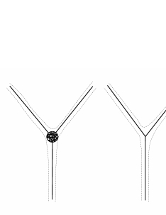
Figure 9: Fixing a length scale, the length between the dashed lines in the sketch above, two different configurations may look the same. A smoothable theory, or ‘non-renormalizable’, is such that the respective solutions converge to a single solution when this scale goes to zero. This can be read in reverse: fixing a scale, we may replace a certain configuration by another whose intersections are all of the most basic type, i.e. whose dual cells are simplices. An example was given by figure 6. Configuration 6a can be viewed as a combination of the ones in 6b and 6c. The error in the two solutions treated as the same thing is smaller the smaller that scale is.

The central property of the secondary manifold is: if $\partial M=\varnothing$ then $\partial W=\varnothing$. Given a division of $M$ into cells, a fixed cell complex, property $\partial W=\varnothing$ is defining $W$. That is, $W$ is a representative of a homology class. $M$ belongs to this class, written appropriately. Given a continuous field $\Psi_{\alpha}$ over $M$ we may associate a dual vertex $\langle\alpha\rangle$ with it and write $M$ isomorphically as $\sum\>\langle\alpha\rangle\times(\textrm{bulk cell})$. This is indeed a $W$. Integrating ${\cal K}$ over this space we get nothing but the usual action evaluated for $\Psi_{\alpha}$. There is a cobordism between this space and any $W$, the smoothing manifold $W^{\alpha}$. Imagine $\Psi_{\alpha}$ approximating better and better a given discontinuous configuration $\Psi_{i}$ as $\alpha\to\infty$. Recall that the fields $\Psi_{i}$ were the starting point for introducing the secondary action $\int_{W}{\cal K}$. Stokes’ theorem allows us to relate it with the usual action for $\Psi_{\alpha}$: they converge to each other iff $\int_{W^{\alpha}}(d+\delta){\cal K}$ vanishes as $\alpha\to\infty$. This is the smoothing theorem II.13. Additionally, there are many other $W$’s in the homology class and many cobordisms $Y$ between them. The different $W$’s can be interpreted as secondary manifolds-remnants of configurations which have been collapsed to the given cell complex. Imagine that it happens that $\int_{Y}(d+\delta){\cal K}=0$ for all cobordisms $Y$. Then the secondary action is independent of which $W$ it is evaluated on i.e. which limiting configuration it is evaluated on, as long as it approaches the fixed cell complex. Configurations of intersecting hypersurfaces are remeniscent of Feynman diagrams and we can make an amusing analogy with properties of quantum field theories. Fixing a length scale, any difference in the value of the action on different configurations which differ below that scale, will be bounded in the order of that scale and go to zero with it. The action does not get ‘renormalized’. An example is sketched in figure 9.

An independent restriction is imposed by requiring diffeomorphism invariance of the action. It is a condition again on $(d+\delta){\cal K}$, theorem V.1. This is a condition essentially complementary to smoothability. Cobordisms $Y$ are extending $W$ in the directions of the dual cells, we deal with dual cells of one dimension higher. Diffeomorphism invariance on the other hand, due to the inner product entering the equations, requires dealing with forms of order 1 higher in the space-time dimensions. Also, for this reason the condition of diffeomorphism invariance is typically somewhat stronger than smoothing.

Once these conditions are satisfied one is in a position to show that $\Psi_{i}$ can indeed be regarded as an exact solution of the equations of motion of the theory. This is possible as conditions are to hold ‘off-shell’. The conditions are typically satisfied if we separate the fields into canonical coordinates and momenta and require continuity in either of the canonical variables. This fact may have some interesting implications in the quantized theory when it makes sense.

Thus the problem posed can be reduced to a question of conditions preserving the cohomology of certain forms, the secondary Lagrangians. I.e. conditions of an essentially topological nature, though we have concerned ourselves only with purely local questions in gravitation. The analogy is between the continua of connections which preserve the Euler number, for example, and the continua of fields $\Psi_{\alpha}$ which approximate a given discontinuous configuration.

Appendix A Conventions

We summarize here basic formulas mentioned in the text and conventions Manes-85 we use: Let $s_{p}$ be a face of a simplex $S$ of dimension $p$ and let $M_{q}$ be a submanifold of $M$ of dimension $q$.

$$s_{p}\times M_{q} =(-1)^{pq}M_{q}\times s_{p},$$

$$\partial(s_{p}\times M_{q}) =\partial s_{p}\times M_{q}+(-1)^{p}s_{p}\times\partial M_{q},$$

Let $\alpha$ be a differential form of degree $(p,q)$ in $(dt,dx)$.

$$\alpha\equiv\alpha_{[p,q]}d^{p}t\wedge d^{q}x =(-1)^{pq}\alpha_{[p,q]}d^{q}x\wedge d^{p}t\,.$$

Integration of $\alpha$ is defined by:

$$\int_{s_{p}\times M_{q}}\alpha=\int_{M_{q}}\left(\int_{s_{p}}\alpha_{[p,q]}d^{p}t\right)d^{q}x.$$

With these conventions Stokes’ theorem is as expected:

$$\int_{s_{p}\times M_{q}}d\alpha=(-1)^{p}\int_{s_{p}\times\partial M_{q}}\alpha,$$

$$\int_{s_{p}\times M_{q}}\delta\alpha=\int_{\partial s_{p}\times M_{q}}\alpha,$$ (76)

$$\Rightarrow\int_{s_{p}\times M_{q}}(d+\delta)\alpha=\int_{\partial(s_{p}\times M_{q})}\alpha.$$ (77)

References

- (1) W. Israel. Singular hypersurfaces and thin shells in general relativity. Nuovo Cim., B44S10:1, 1966. Erratum, Nuovo Cim. B48 (1967) 463.
- (2) G. Hayward and J. Luoko. Variational principles for non-smooth metrics. Phys. Rev. D, 42:4032, 1990.
- (3) S. W. Hawking. The path integral approach to quantum gravity. In S. W. Hawking and W. Israel, editors, General Relativity: An Einstein Centenary Survey, page 746. Cambridge University Press, 1979.
- (4) C. J. Isham. Some Quantum Field Theory Aspects of the Superspace Quantization of General Relativity. Proc. Roy. Soc. Lond., A351:209, 1976.
- (5) Roland Steinbauer and James A. Vickers. The use of generalised functions and distributions in general relativity. Class. Quant. Grav., 23:R91–R114, 2006.
- (6) R. Geroch and J. H. Traschen. Strings and other distributional sources in general relativity. Phys. Rev., D36:1017, 1987.
- (7) D. Lovelock. The einstein tensor and it’s generalisations. J. Math. Phys., 12:498–501, 1971.
- (8) Dmitri V. Fursaev and Sergey N. Solodukhin. On the description of the Riemannian geometry in the presence of conical defects. Phys. Rev., D52:2133–2143, 1995.
- (9) Nathalie Deruelle and Cristiano Germani. Smooth branes and junction conditions in Einstein Gauss- Bonnet gravity. Nuovo Cim., 118B:977–988, 2003.
- (10) E. Gravanis and S. Willison. ‘Mass without mass’ from thin shells in Gauss-Bonnet gravity. Phys. Rev., D75:084025, 2007.
- (11) E. Gravanis and S. Willison. Intersecting hyper-surfaces in dimensionally continued topological density gravitation. J. Math. Phys., 45:4223–4238, 2004.
- (12) E. Gravanis and S. Willison. Intersecting hypersurfaces, topological densities and Lovelock gravity. J. Geom. Phys., 57:1861–1882, 2007.
- (13) Alex Giacomini, Ricardo Troncoso, and Steven Willison. Junction conditions in general relativity with spin sources. Phys. Rev., D73:104014, 2006.
- (14) Steven Willison. Intersecting hypersurfaces and Lovelock gravity. PhD thesis, Kings College London, 2004.
- (15) T. Regge. On broken symmetries and gravity. Phys. Rept., 137:31–33, 1986.
- (16) A. Mardones and J. Zanelli. Lovelock-cartan theory of gravity. Class. Quant. Grav., 8:1545, 1991.
- (17) C. Nash. Differential Topology and Quantum Field Theory. Academic Press, 1991.
- (18) S. S. Chern and J. Simons. Characteristic forms and geometric invariants. Annals Math., 9:48–69, 1974.
- (19) S. S. Chern. Complex manifolds without potential theory. Springer-Verlag, New York, 1995.
- (20) B. Huo H. Guo, K. Wu and S. Wang. Anomalies, cohomology and generalised secondary classes. In Moscow, “Quantum gravity”, page 165, 1984.
- (21) R. Stora J. Manes and B. Zumino. Algebraic study of chiral anomalies. Commun. Math. Phys., 102:157, 1985.
- (22) L. Alvarez-Gaume and P. Ginsparg. The structure of gauge and gravitational anomalies. Annals Phys., 161:423, 1985. Erratum-ibid. 171, 233 (1986).
- (23) William S. Massey. A Basic Course in Algebraic Topology. Springer-Verlag, 1991.
- (24) Christos Charmousis and Robin Zegers. Matching conditions for a brane of arbitrary codimension. JHEP, 08:075, 2005.
- (25) Robin Zegers. Self-gravitating branes of codimension 4 in Lovelock gravity. JHEP, 03:066, 2008.
- (26) Allen Hatcher. Algebraic Topology. Cambridge University Press, 2002.