Active region transition region loop populations
and their relationship to the corona

Abstract

The relationships among coronal loop structures at different temperatures is not settled. Previous studies have suggested that coronal loops in the core of an active region are not seen cooling through lower temperatures and therefore are steadily heated. If loops were cooling, the transition region would be an ideal temperature regime to look for a signature of their evolution. The Extreme-ultraviolet Imaging Spectrometer (EIS) on Hinode provides monochromatic images of the solar transition region and corona at an unprecedented cadence and spatial resolution, making it an ideal instrument to shed light on this issue. Analysis of observations of active region 10978 taken in 2007 December 8 – 19 indicates that there are two dominant loop populations in the active region: core multi-temperature loops that undergo a continuous process of heating and cooling in the full observed temperature range $0.4-2.5$ MK and even higher as shown by the X-Ray Telescope (XRT); and peripheral loops which evolve mostly in the temperature range $0.4-1.3$ MK. Loops at transition region temperatures can reach heights of 150 Mm in the corona above the limb and develop downflows with velocities in the range of $39-105\,\rm km\,s^{-1}$.

1 Introduction

Loop structures in the Solar corona have been observed at temperatures spanning several thousand to several million K. Lately considerable effort has gone into understanding the relationship among these structures. Despite these efforts, we have not yet developed a fully coherent picture of how structures at different temperatures are related. One of the goals is to understand whether these are independent structures governed by different heating mechanisms with different temporal and spatial characteristic scales, or whether they are just snapshots of the same structures in different stages of their evolution.

We do know that active regions do not look exactly the same in different temperature regimes. The core of the active region is generally dominated by hot, high density loops. Electron temperatures in an active region core are typically near 3 MK (e.g. Saba & Strong, 1991; Brosius et al., 1997). The footpoints of these hot loops form the “moss”, which is the bright network pattern observed in emission lines formed near 1 MK (Berger et al., 1999). The periphery of the active region is generally dominated by longer loops with lower temperatures (Del Zanna & Mason, 2003).

The relationship between the hot core loops and the “warm” loops has not been completely established. In fact, it has been proposed that they are largely independent. Antiochos et al. (2003) argued that soft X-ray loops in the cores of active regions are not seen cooling to lower temperatures in filter images, therefore implying a steady source of heating (see also Martens, 2008), and some success has been achieved in modeling such a scenario (Winebarger et al., 2008; Warren et al., 2008). It is evident from other observations, however, that many soft X-ray active region loop structures cool down and are observed in the EUV at 1 – 2.5 MK (Winebarger & Warren, 2005; Ugarte-Urra et al., 2006; Warren et al., 2007). The open question is which is the dominating component and what role do observational constraints, such as spatial resolution, play in that apparent steadiness. No observational study has given a fully satisfactory answer to this question yet.

If coronal loops are cooling, it seems natural to look for signatures of the evolution at lower temperatures. The relationship of the hot and warm loops to structures at temperatures between 0.1 and 1 MK, traditionally called transition region temperatures, is however unclear. To the complex nature of the transition region (e.g. Mariska, 1992) we have to add the fact that even though images of the corona have been routinely taken by Soft X-ray (e.g. SXT/Yohkoh, XRT/Hinode) and Extreme Ultra-Violet (e.g. EIT/SOHO, TRACE, EUVI/STEREO) imagers for many years now, that has not been the case for temperatures between 0.1 and 0.8 MK. Our understanding of this important and very dynamic component of the atmosphere is mostly based on spectroscopic observations, which often lack simultaneous good spatial and temporal sampling. Spectroscopic images take several minutes, sometimes hours, to build up, while sit-and-stare time series lack context. The latest best efforts for their high spectral and spatial resolution and sensitivity have been made with the CDS and SUMER spectrometers on board SOHO. Observations have shown that loop structures are common at transition region temperatures and that they reach heights (100 Mm) usually associated with coronal plasmas (e.g. Brekke, 1999). These loops are nearly complete or consist of long segments, suggesting isothermality (Fredvik et al., 2002; Chae et al., 2000). Sometimes they form condensations, also seen by TRACE (Schrijver, 2001), and they are characterized by their short-term variability on the order of tens of minutes (Kjeldseth-Moe & Brekke, 1998; Fredvik et al., 2002).

These studies, however, failed to reach a definite conclusion on the relationship of these structures to higher temperature coronal plasmas (Brekke, 1999). On the one hand, the co-spatiality and co-temporality of loops at multiple temperatures was reported (e.g. Kjeldseth-Moe & Brekke, 1998; Spadaro et al., 2000; Schmelz & Martens, 2006). On the other, authors like Fludra et al. (1997) have stated that the evolution of plasma with temperatures under 0.6 MK is independent of the evolution of the coronal plasma. In similar terms, Matthews & Harra-Murnion (1997) and Harra-Murnion et al. (1999) have also concluded that high lying cool loops are not the result of the cooling of hot loops, but rather that they are separate co-existing entities. The lack of connection between active region emission in the transition region and the corona was also discussed by other authors (Feldman & Laming, 1994; Landi & Feldman, 2004). Despite their conclusions, some of these studies acknowledged the difficulty of interpreting simultaneous images at different temperatures, which leaves open the possibility that these transition region loops may be the result of the cooling of hot structures (e.g. Strong & Bruner, 1996; Harra et al., 2004).

At this crossroads, we present an initial analysis of transition region imaging from the Extreme-ultraviolet Imaging Spectrometer (EIS) on board Hinode, to clarify some of the open questions raised by these earlier studies. In addition to the 1″ and 2″ narrow slits, EIS also has a 40″ slot. This slot allows EIS to image the Sun over relatively narrow ($\approx$1 Å) wavelength ranges. The broad range of temperatures in the EIS wavelength ranges provide monochromatic images in lines ranging from Mg VI to Fe XVI. The EIS slot images are similar to those taken with the Skylab S082A instrument (Tousey et al., 1977), except that the blending is significantly reduced: images subtend 1 Å on the detector versus the 25 Å in Skylab. The field of view is limited, but larger fields of view can be imaged by stepping the slot across the region of interest.

Our main conclusions, in Section 4, are that active regions have, at least, two main loop populations: the core loops that are energized to several million K and cool down to transition region temperatures; and the peripheral cool loops that have peak emissions in the range $0.4-1.3$ MK. The nature as well as the temporal and spatial characteristics of the heating of these structures still remain to be determined. More details on the loop results are given in Section 3. First, we introduce in Section 2 the EIS spectrometer, the set of observations and why they are of interest.

2 Observations

2.1 EIS observing and mode selection

The EUV Imaging Spectrometer (EIS) (Culhane et al., 2007) on Hinode (Kosugi et al., 2007) is a flexible spectrometer which can be used in three main modes of operation. Firstly, using the 1″ or the 2″ slits, it can simply retrieve a sequence of spectra of the same solar location to allow the study of its full spectral properties at consecutive times. Secondly, using the same slits and a scan motion it can retrieve a sequence of spectra at adjacent solar positions to study the full spectral properties of an extended region, up to $590\arcsec\times 512\arcsec$. In the first mode, temporal resolution is gained at the expense of spatial extension and the opposite occurs in the second mode. Intermediate configurations allow a compromise between the two. In these two modes, the spectroscopic capabilities are normally prioritized over spatial and temporal sampling.

EIS also allows us to trade part of the spectral capabilities to improve the cadence and field-of-view coverage, giving the former three properties almost equal importance. This can be accomplished by using the 40″ (also 266″) aperture, also called the slot. Each spectral line then produces its own 40″ image. As a result the detector hosts as many images as there are spectral lines in the wavelength range. Images produced by spectral lines with centroids closer than 40 spectral pixels (one spectral pixel corresponds to 1″ on the Sun) will overlap and be difficult to interpret. There are, however, many spectral lines that are sufficiently isolated from neighboring strong lines. For those lines EIS can achieve imaging capabilities comparable to those of EUV imagers, at a greater spectral, and therefore temperature discrimination. Single exposures cover as much as $40\arcsec\times 512\arcsec$ and require shorter exposure times than the narrow slits, which allows better temporal sampling. The trade off to obtain these fast spectrally pure images is an overlap of spectral and spatial information and, therefore, the loss of a fully resolved spectrum that could be subject to the usual spectral analysis: line fitting, etc. Similar modes of operation have already been used in the past, e.g. Skylab spectroheliograms (e.g. Tousey et al., 1973) or slot images with the Coronal Diagnostic Spectrometer on board SOHO (e.g. Ugarte-Urra et al., 2004). EIS’s novelty is its improved sensitivity, spectral coverage and spatial resolution.

2.2 Active region NOAA 10978

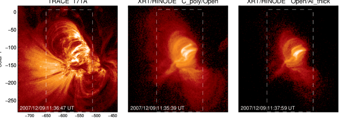
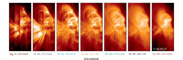
Figure 1: Active region NOAA 10978 as seen by an EUV and an X-Ray imager (TRACE and XRT/Hinode), top panels, and as seen by EIS slot imaging. The center graph indicates the temperature response of the different instruments.

Interested in the relationships among loops at different temperatures and aware of the unique capabilities of the EIS for spectral imaging, our aim was to take a fresh look at the evolution of active region loop structures in unprecedented detail. Our goal was then to look at them in a similar way to that which has been done with EUV imagers, but taking advantage of the temperature discrimination that the slot images provide. Fig.1 shows the temperature response of the EIS slot images (color solid lines) in comparison to three TRACE and XRT passbands (dotted lines). The lines on the graph represent the temperature range where lies 95% of the contribution funcion of the spectral lines in the case of EIS and 95% of the temperature response in the case of TRACE and XRT.

We therefore planned a 12 day run of observations of active region (AR) NOAA 10978 with long sequences of slot imaging, while the AR rotated from the East to the West limb. The study basic unit consisted of four $40\arcsec\times 400\arcsec$ exposures of 15 seconds at four adjacent solar positions with a 5″ overlap, resulting in a $140\arcsec\times 400\arcsec$ region sampled every 70 seconds in eighteen different spectral lines. Spectral lines were chosen for their spectral purity and temperature coverage, see Table 1, assessed in previous full CCD observations. It is worth noting the presence of three purely transition region lines: Mg VI ($\rm T\approx 0.4\,MK$), Mg VII and Si VII ($\rm T\approx 0.6\,MK$). Studying the evolution of loop structures in spectrally pure images (isothermal plasma) of the transition region and the corona at a 70 s cadence should be sufficient to establish the, heretofore unclear, relationship between plasmas at those temperatures and timescales. By isothermal we mean a temperature response as narrow as the width of the line transition’s contribution function (e.g. Mariska, 1992).

AR 10978 (Fig. 1) appeared over the East limb on December 4, 2007. It was a moderately sized active region that, on its passage towards the West limb, experienced moderate activity in terms of GOES fluxes. As shown in Fig. 2, ten C-flares are associated with its development during the twelve days observing time. The figure also indicates (Greek symbols) the magnetic classification of AR 10978 as given by NOAA. The index gives a notion of activity in the active region (e.g. Ireland et al., 2008). Dalla et al. (2007) investigated a sample of 2880 sunspot regions from the NOAA Solar Region Summary catalog and found that 73% of active regions have $\beta$ as maximum magnetic classification and 11% reach $\beta\gamma$. As shown in Fig. 2 AR 10978 belongs to the latter group, i.e. a bipolar sunspot group with more than one clear north-south polarity inversion line.

The data were reduced using standard EIS software. The slot images, similarly to narrow slit observations, experience a drift on the detector due to the satellite orbital changes (Brown et al., 2007). This is corrected via cross-correlation of consecutive images, which also removes the spacecraft jitter.

3 Active region transition region emission and loop population

Our study of several hours a day for a 12 day observing sequence of multi-wavelength slot movies reveals that active regions can exhibit transition region contributions from two distinct loop populations: compact multi-temperature core loops and cool and extended peripheral loops. Other significant contributors are active region transition region brightenings and an unresolved low lying component. Although the individual contribution of all these parts has been reported before, (see introduction papers and references therein, and Young et al., 2007, for EIS initial results), we will give a further insight into their relationship with other structures seen at different temperatures. Our emphasis will be towards the two distinct loop populations.

3.1 Compact multi-temperature loops

To the trained eye in EUV coronal loop observations, the most novel and noticeable features in the slot movies are transition region loops characterized for being short lived and clearly defined along their full length (or a large portion of it). Loops with similar characteristics were already observed with CDS (Brekke, 1999). They connect footpoints at both sides of the neutral line in the same way the hot coronal emission does. An easy proxy of their locii in the current dataset is the envelope of the AR core and diffuse emission in the C_poly XRT image in Fig.1. Therefore, one first thing to notice is that they occur where hot emission ($\geq$2.5MK, i.e. Fe XVI) is present.

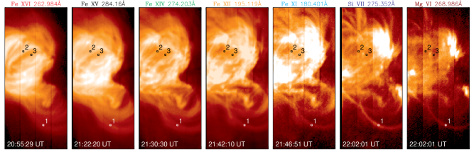
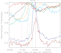
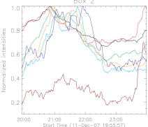
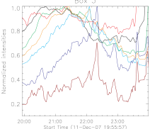
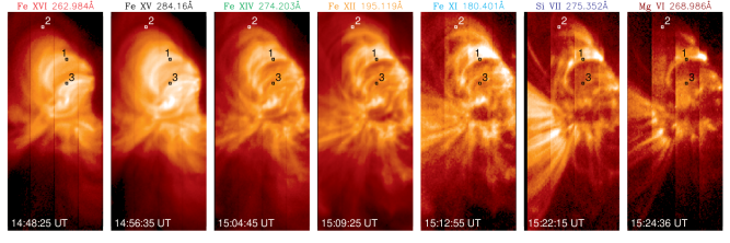
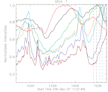
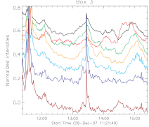
Figure 3: Compact multi-temperature loops. Normalized intensity lightcurves for several spectral lines at three different locations: boxes 1, 2 and 3. Top half corresponds to December 11 2007 observing time and bottom half to December 9 2007. Times of slot images correspond to dashed lines on box 1 lightcurves, i.e. peak in intensity. Integration boxes are 3$\times$3 pixels. For the sake of clarity, all the curves (but box 3 in December 9) have been smoothed with a boxcar average of 3 data points in time and an absolute value of 0.3 has been subtracted of the Mg VI curves.

Their relationship with structures at higher temperatures becomes evident when plotting lightcurves of the intensity of different spectral lines with different formation temperatures. The lightcurves indicate that these transition region loops are the result of cooling of multi million degree plasma. Fig.3 shows examples for December 11 (top half) and December 9 (bottom half). The lightcurves, in normalized intensities, are shown for three different locations on the active region (boxes 1, 2 and 3). Different spectral lines are indicated in different colors (see color coding on the figure). On top of the lightcurve panels we show context composite slot images for all these spectral lines at the time of maximum intensity in box 1, dashed lines on box 1 lightcurve panel. These slot images are available as movies in the online version of the paper.

The loop under box 1 on December 11 is a good example. The loop is first observed at temperatures $\geq 2.5$ MK (Fe XVI) and slowly cools down through all the spectral lines sampled by EIS. It takes approximately 65 minutes to reach a maximum in intensity at transition region temperature (Si VII) and its identification is unambiguous at all temperatures. The other boxes show similar general patterns except for transient brightenings (e.g. box 3 on December 9 13:30 UT) which will be discussed later on.

Loops clearly seen at transition region temperatures can sometimes be difficult to identify in Fe XV - XVI images due to the higher background and foreground emission, interpreted as a larger population of loops at those temperatures at any instant in time. This is better quantified by stating that the contrast of the loops to the background emission ranges 1.4 – 2.0 in Fe XV, 1.7 – 4.0 in Fe XII and 2.2 – 5.8 in Si VII.

As seen in the two examples in Fig.3, these transition region loops emit along their full length or a big fraction of it, suggesting isothermality along the structures at any given instant. The lightcurves, however, show an evident overlap at different temperatures, which also suggests that the thermal distribution has a certain width. We present an emission measure analysis of this active region elsewhere (Warren et al., 2008). Results indicate that the thermal distribution along the line-of-sight has a typical width of $\approx 3\times 10^{5}$ K. It is important to note here that we do not see transition region loops, as described in this section, that do not reach coronal temperatures.

Lifetimes at transition region temperatures are on the order of tens of minutes. Table 2 gives lifetime estimates for a sample of several loops that were background subtracted in coronal and transition region lines. The lifetime is defined as the full width at half maximum intensity. Evolution times are longer for coronal lines. This is also reflected in the smoothness of the lightcurves that increases for larger temperatures. The smooth envelopes of coronal emission can often be associated with several cooler events. This has been seen before in different scenarios, and together with the fact that loops appear to live longer than their characteristic cooling time, has lead some authors to consider multiple threads as an important part of loop evolution at this resolution (e.g. Warren et al., 2002; Warren et al., 2003).

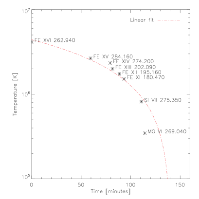
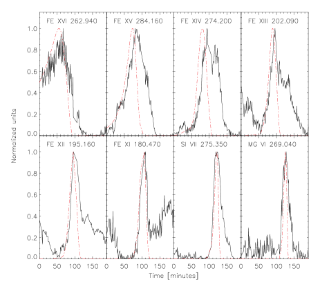
Figure 4: Left panel: Temperature decay as a function of time for the loop under box 1 on December 11. Right panel: normalized background subtracted intensity lightcurves in solid black and variation of the contribution function as function of time and temperature change in red dot-dashed line.

The current dataset is one of the most complete in terms of temperature coverage for a loop evolution and this issue can be investigated with some detail. The left panel on Fig. 4 shows the estimated temperature decay for the loop that lies underneath box 1 on December 11. Each datapoint represents the time when the loop’s lightcurve for that specific spectral line reaches half its peak intensity in the rising phase, and the temperature where we expect that spectral line to become observable. We arbitrarily define it as the largest temperature where the atomic contribution function of the spectral line is larger than half its maximum. The red dot-dashed line corresponds to the linear fit to those points. Even though an exponential fit can be a fair approximation of the decay in the range 1.5 – 3 MK, the linear fit reproduces better the observations in the overall temperature range. The right panel in the figure shows in black the normalized background subtracted intensities for that loop as function of time. The red dot-dashed curves represent the variation in time of the spectral line contribution function assuming the temperature changes indicated by the linear fit. The contribution function is proportional to the emissivity of the line, i.e. it is a proxy of the loop’s lightcurve. This plot shows that the observed loop’s lifetime can be very close to the expected one from the characteristic cooling time given by the fits. This is the case for some of the cooler lines. There are large inconsistencies, however, for other lines that have slow intensity decay tails. It is not clear therefore that lifetimes and lightcurves can be fully explained by the cooling rate. A study of a statistically significant sample should give us more insight in whether the discrepancies are systematic.

Another interesting note on these loops is that sometimes they recur, i.e. a loop with similar topology goes through several cycles of (heating and) cooling. An example is box 1 lightcurve on December 9. The behavior has been reported before (Shimizu, 1995; Ugarte-Urra et al., 2006).

These properties are true in the quietest period between days 8 and 12 (see Fig. 2), and become more evident when flaring activity steepens up on days 12, 13 and 14. During those days the active region is observed on-disk. Off-limb (December 19) the picture becomes more confusing, as the emission from loops in the core lies in the same line-of-sight as the legs of long peripheral loops described in the next section. Furthermore, the contribution from foreground and background emission at 1-2 MK in the core is larger off-limb, as we integrate through twice the contribution: both legs versus just loop tops on-disk. Individual loops can still be pinpointed in the transition region lines, but their relationship to hotter temperatures is not as clear. This would explain partly why CDS studies, many off-limb, resulted in different conclusions. Another reason is that those studies did not have the spectral coverage at the temporal cadence that EIS slot movies provide.

3.2 Peripheral extended cool loops

A second distinct population of loops is located at the periphery of the active region core. In Fig. 1 these loops are the ones that are visible in the lower left quarter of the TRACE 171 Å image, but not at the same location in XRT. In EIS slot images those loops are most prominent in Si VII and Mg VII, which correspond to a temperature of 0.6 MK in ionization equilibrium, below the temperature of maximum response of the 171 Å passband. Their cool nature was already diagnosed using the spectroscopic capabilities of CDS (Del Zanna & Mason, 2003; Del Zanna, 2003) and more recently EIS (Young et al., 2007). Those studies lack temporal information and justify our investigation of the temporal evolution of the loops. Our analysis confirms that the main contribution to these loops over time is in the range 0.4 – 1.3 MK. Unlike the loops described in Section 3.1, these loops do not seem to be the result of cooling of $\geq$2.5 MK loops.

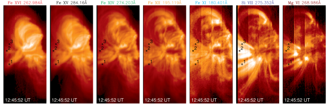
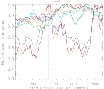
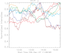
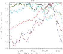
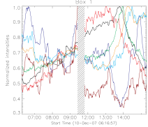
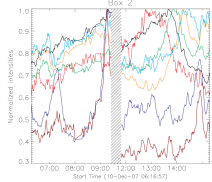
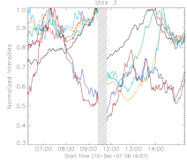
Figure 5: Peripheral cool loops. Filled pattern indicates there is a data gap of approximately 2.4 hours. Notice times on the abscissa axis. For the sake of clarity, all the curves have been smoothed with a boxcar average of 3 data points in time. There is very little correspondence between intensity changes at transition region temperatures and the corona.

Fig. 5 shows lightcurves for representative locations on two different days, December 9 (top) and December 10 (bottom). Notice there is a data gap of 2.4 hours on December 10 (filled pattern) due to EIS operational constraints. The intensity lightcurves from loop structures at 0.4 and 0.6 MK (respectively in blue and brown colors, Mg VI and Si VII) are correlated. Yet, in contrast to the lightcurves in Fig.  3, there is not such a clear cut correspondence between the intensity changes at transition region temperatures and the changes in lines formed at higher coronal temperatures. The lightcurves suggest that loops at transition region and lower coronal temperatures evolve independently of the hotter structures. In some instances, like December 9 box 2 between 13:00 UT and 14:00UT, the enhancements in the Si VII and Mg VI lightcurves (and movies) can be associated to earlier changes in Fe XI and Fe XII, suggesting that these loops could well reach temperatures up to 1.3 MK. However, our analysis does not give any indication that these loops reach the formation temperatures of Fe XIV – Fe XVI. Lightcurves of boxes 1, 2 an 3 on December 10 do show in several instances a similar pattern of cooling as described in the previous section, however, a close inspection of the movies reveals that this is the result of line-of-sight contamination from multi-temperature loops and can not be interpreted as a characteristic evolution of the background peripheral loops.

The Si VII and Mg VI lightcurves reveal structuring within the smoother general trends, for example in box 3 (December 9). The time scales for these structures is on the order of tens of minutes and it is likely that some of these changes are oscillatory in nature. Further work is in progress to investigate it. The loops are clearly visible as fan structures in TRACE 171 Å and the presence of waves in this type of loops is a well documented phenomenon (e.g. De Moortel et al., 2002, and references therein).

3.3 Off-limb emission

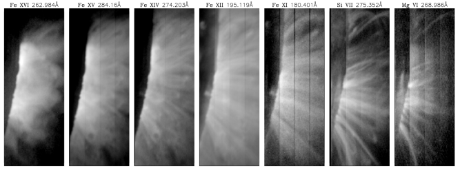
Figure 6: Active region loops as seen on projection over the West limb in various different spectral lines, covering a temperature range of 2.5 MK - 0.4 MK. Time: 07:09 UT, December 19 2007.

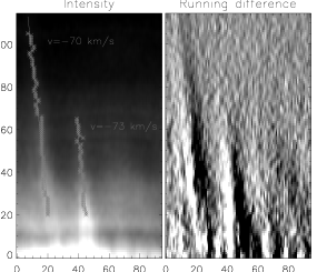
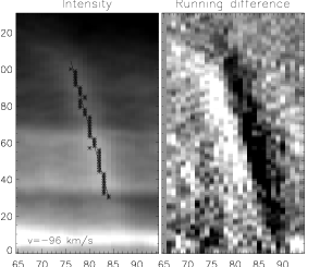
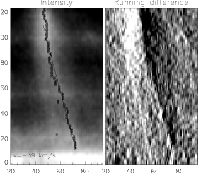
Figure 7: Downflows along the legs of three different Mg VI off-limb loops. Asterisks indicate the maximum of the intensity in the lightcurve at a given location along the loop’s axis. Solid lines are linear fits to the points. The slope of the curve is the associated velocity. Exposure 0 corresponds to time 05:55 UT, December 19 2007.

Emission at the coolest temperatures in the dataset is not just constrained to the footpoints, but it extends into coronal heights. That is best seen in projection over the limb. Fig. 6 shows an image of the active region on December 19 over the West limb. As pointed out earlier, off-limb images have a large line-of-sight contamination, mostly at coronal temperatures. In the cooler lines, some loops can be clearly isolated. Their legs extend as much as 150 Mm and more interestingly the intensity changes, mostly in Mg VI, indicate the presence of downflows along the legs towards the surface. These downflows are also noticeable on-disk. On projection over the plane of the image, the velocities are in the range $39-105\,\rm km\,s^{-1}$. Fig. 7 shows various examples of downflows in three different loops. The plots represent the change of intensity along the loop’s axis in time, with the limb at the bottom. The intensities have been smoothed in a boxcar of 2 pixels to reduce noise. Running differences are shown to enhance the downflow path. Asterisks indicate the maximum intensity in time at a particular position along the axis. The velocities result from the linear fit to these points. This phenomenon has been referred to as coronal rain (Foukal, 1978) and it appears to be a rather common process in active regions interpreted in terms of catastrophic cooling of the loops (Schrijver, 2001; Müller et al., 2005; Karpen et al., 2006). Simultaneous Ca II H images from the Solar Optical Telescope on board Hinode, show clumps of material continuously falling at chromospheric temperatures off-limb.

3.4 Transition region brightenings and the unresolved component

Sudden (few frames) brightenings are another contributor to transition region emission. They tend to be point-like, but they can be elongated too. At the movies cadence (70 s) these events brighten up simultaneously at several temperatures. Sometimes they reach up to Fe XVI temperatures, some other times they seem constrained to the cooler spectral lines. Their impulsiveness does not allow to resolve their temperature evolution at this cadence, which makes them distinct from the other discussed loop samples. One example is the sudden intensity increase seen in box 3 on December 9 13:26 UT at all temperatures. The magnetic changes associated with them appear different from the ones associated with the clearly defined loops described in previous sections (Brooks et al., 2008). The dimensions of these events are often close to the spatial resolution of the spectrometer. Earlier studies have already discussed the properties of active region transient events that reach coronal temperatures (Shimizu, 1995; Berghmans et al., 2001, and references therein) and events that remain cooler (namely explosive events, e.g. Pérez et al., 1999). We should stress however that the majority of transient events described by Shimizu (1995) present a single loop or multiple loop morphology and lifetimes which are also consistent with the loop population described in Section 3.1. In fact, transient X-ray loops have been seen cooling in the EUV (Ugarte-Urra et al., 2006; Warren et al., 2007). Therefore, we believe that observations with higher spatial and temporal resolution would be needed to investigate if these sudden unresolved transient coronal brightenings are different in nature (Brooks et al., 2008) to the transient loops described in Section 3.1.

Finally, and for completeness, there is also a transition region contribution from an unresolved component, which we will not discuss further in this paper. The origin of this component could be associated with the footpoints of coronal loops, the thermal interface in a continuous stratified atmosphere (e.g. Griffiths et al., 2000), or to unresolved cool structures disconnected from the corona (e.g. Landi & Feldman, 2004).

4 Discussion and conclusions

Our investigation of monochromatic images and movies of the solar atmosphere taken with the Extreme-ultraviolet Imaging Spectrometer at an unprecedented cadence and spatial resolution gives new clues about the relationship between loop structures seen in different temperature regimes at different times.

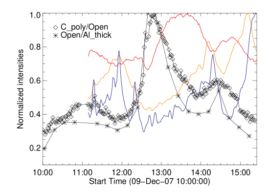
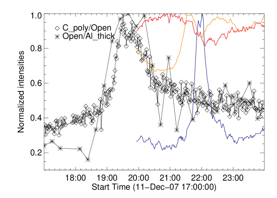
Figure 8: XRT Box 1 lightcurves for two filter combinations (diamonds and asterisks) on December 9 and 11. Fe XVI, Fe XII and Si VII lightcurves also shown for comparison with Fig 3. Same color coding as that figure.

We find that loops in the core of the active region experience a heat deposition that makes them reach temperatures at least as high as 2.5 MK, which is then followed by a cooling process down to transition region temperatures, as low as the temperature response of the coolest spectral line in the dataset (0.4 MK). The process can recur in a time-span of several hours. In fact, the temperatures reached by these loops are probably higher. We have investigated the soft X-ray lightcurves (XRT) (Golub et al., 2007) of a few examples and soft X-ray enhancements precede the EUV response. Fig. 8 shows the XRT C_poly$/$Open and Open$/$Al_thick filter combination lightcurves for Box 1 on December 9 and 11. The peak in the temperature response for those filters is 8 and 12 MK respectvely. This is in agreement with our previous studies (Ugarte-Urra et al., 2006; Warren et al., 2007) and indicates that there is a non-negligible component of loops in active regions that undergo a continuous heating and cooling process.

The loops emit along their full length, or a big fraction of it, at all temperatures. Together with the fact that the thermal distribution has a typical width of $\approx 3\times 10^{5}$ K (Warren et al., 2008) this suggests that at any given instant in time, loops are isothermal structures, possibly filamented, with a cross-field coherence.

Previous studies (Fludra et al., 1997; Matthews & Harra-Murnion, 1997; Harra-Murnion et al., 1999) have suggested that there is a population of transition region loops reaching coronal heights evolving independently from the coronal plasmas. At the core we do not find evidence of loops at transition region temperatures that are not the result of cooling from multimillion degree plasma. The evolution of these cool loops is associated with the cooling of coronal structures. At the core’s periphery, however, we do observe loops with their major contribution in the range $0.4-1.3$ MK and we do not find evidence in our datasets that these loops result from the cooling of multimillion degree plasmas. This result confirms previous spectroscopic diagnostics of the loops.

These two populations are the dominant components of the coronal and transition region emission during the full week passage of the active region and as such have to be explained by any physical model. It remains to be proved, however, that these populations prevail in every active region. In fact, that it is probably not the case, as the existence of a much steadier multi-million K loop population has been reported in the past (e.g. Antiochos et al., 2003). Given the proposed scenarios for coronal heating, e.g. magnetic braiding and reconnection, it is likely that the level of magnetic complexity at the photospheric level is related to the soft X-ray and EUV response in the atmosphere. We have shown that this active region has a magnetic classification ($\beta\gamma$) that would put it among a minority (11%) of observed active regions (Dalla et al., 2007). Therefore, future investigations should address the relationship between loop evolution and magnetic complexity in an attempt to identify and characterize the various mechanism at play that result in the distinct loop populations and their evolution.

Table 1: Spectral lines

Ion		Wavelength [Å]	T [MK]
He	II	256.3	0.05
Mg	VI	269.0	0.40
	VII	278.4	0.63
Si	VII	275.4	0.63
	X	258.4	1.26
	X	261.1	1.26
Fe	XI	180.5	1.26
	XI	188.3	1.26
	XII	195.2	1.26
	XIII	202.1	1.58
	XIII	203.9	1.58
	XIV	211.3	2.00
	XIV	274.2	2.00
	XV	284.2	2.00
	XVI	251.1	2.51
	XVI	262.9	2.51
	XXIII	264.0	15.85
Ca	XVII	192.8	5.01

Figure 2: GOES 1-8 Å fluxes during the observing period. Flare class is indicated by the dashed lines and M, C, B letters. Greek letters indicate AR10978 magnetic classification given by NOAA.

Table 2: Sample of loop lifetimes

		Fe XV		Fe XII		Si VII		Mg VI
No.	Date	Start Time	Lifetime	Start Time	Lifetime	Start Time	Lifetime	Start Time	Lifetime
1	2007/12/09	13:53:35	770s	14:06:24	630s	14:16:55	770s	14:18:05	770s
2	2007/12/09	14:36:45	770s	14:43:46	560s	14:44:55	560s	14:44:55	560s
3	2007/12/10	13:54:53	1820s	14:10:04	1050s	14:17:04	840s	14:19:23	770s
4	2007/12/10	13:56:02	1261s	14:05:23	980s	14:06:34	840s	14:07:43	770s
5	2007/12/11	07:23:45	1470s	07:38:55	840s	07:43:35	1121s	07:44:45	981s
6	2007/12/11	20:49:40	3431s	21:24:40	1540s	21:49:10	1121s	21:52:41	1190s
7	2007/12/12	19:51:51	1961s	20:18:41	1330s	20:28:01	1332s	20:29:12	1191s
8	2007/12/12	20:42:02	1786s	21:05:24	1226s	21:22:20	1190s	21:24:39	1120s
9	2007/12/13	21:04:13	4165s	21:39:16	1993s	22:27:40	1820s	-	-

References

- Antiochos et al. (2003) Antiochos, S. K., Karpen, J. T., DeLuca, E. E., Golub, L., & Hamilton, P. 2003, ApJ, 590, 547
- Berger et al. (1999) Berger, T. E., de Pontieu, B., Schrijver, C. J., & Title, A. M. 1999, ApJ, 519, L97
- Berghmans et al. (2001) Berghmans, D., McKenzie, D., & Clette, F. 2001, A&A, 369, 291
- Brekke (1999) Brekke, P. 1999, Sol. Phys., 190, 379
- Brooks et al. (2008) Brooks et al. 2008, Submitted to ApJ
- Brosius et al. (1997) Brosius, J. W., Davila, J. M., Thomas, R. J., Saba, J. L. R., Hara, H., & Monsignori-Fossi, B. C. 1997, ApJ, 477, 969
- Brown et al. (2007) Brown, C. M., et al. 2007, PASJ, 59, 865
- Chae et al. (2000) Chae, J., Wang, H., Qiu, J., Goode, P. R., & Wilhelm, K. 2000, ApJ, 533, 535
- Culhane et al. (2007) Culhane, J. L., Harra, L. K., James, A. M., Al-Janabi, K., Bradley, L. J., Chaudry, R. A., Rees, K., Tandy, J. A., Thomas, P., Whillock, M. C. R., Winter, B., Doschek, G. A., Korendyke, C. M., Brown, C. M., Myers, S., Mariska, J., Seely, J., Lang, J., Kent, B. J., Shaughnessy, B. M., Young, P. R., Simnett, G. M., Castelli, C. M., Mahmoud, S., Mapson-Menard, H., Probyn, B. J., Thomas, R. J., Davila, J., Dere, K., Windt, D., Shea, J., Hagood, R., Moye, R., Hara, H., Watanabe, T., Matsuzaki, K., Kosugi, T., Hansteen, V., & Wikstol, Ø. 2007, Sol. Phys., 243, 19
- Dalla et al. (2007) Dalla, S., Fletcher, L., & Walton, N. A. 2007, A&A, 468, 1103
- De Moortel et al. (2002) De Moortel, I., Ireland, J., Hood, A. W., & Walsh, R. W. 2002, A&A, 387, L13
- Del Zanna (2003) Del Zanna, G. 2003, A&A, 406, L5
- Del Zanna & Mason (2003) Del Zanna, G., & Mason, H. E. 2003, A&A, 406, 1089
- Feldman & Laming (1994) Feldman, U., & Laming, J. M. 1994, ApJ, 434, 370
- Fludra et al. (1997) Fludra, A., Brekke, P., Harrison, R. A., Mason, H. E., Pike, C. D., Thompson, W. T., & Young, P. R. 1997, Sol. Phys., 175, 487
- Foukal (1978) Foukal, P. 1978, ApJ, 223, 1046
- Fredvik et al. (2002) Fredvik, T., Kjeldseth-Moe, O., Haugan, S. V. H., Brekke, P., Gurman, J. B., & Wilhelm, K. 2002, Advances in Space Research, 30, 635
- Golub et al. (2007) Golub, L., et al. 2007, Sol. Phys., 243, 63
- Griffiths et al. (2000) Griffiths, N. W., Fisher, G. H., Woods, D. T., Acton, L. W., & Siegmund, O. H. W. 2000, ApJ, 537, 481
- Harra-Murnion et al. (1999) Harra-Murnion, L. K., Matthews, S. A., Hara, H., & Ichimoto, K. 1999, A&A, 345, 1011
- Harra et al. (2004) Harra, L. K., Mandrini, C. H., & Matthews, S. A. 2004, Sol. Phys., 223, 57
- Ireland et al. (2008) Ireland, J., Young, C. A., McAteer, R. T. J., Whelan, C., Hewett, R. J., & Gallagher, P. T. 2008, ArXiv e-prints, 805
- Karpen et al. (2006) Karpen, J. T., Antiochos, S. K., & Klimchuk, J. A. 2006, ApJ, 637, 531
- Kjeldseth-Moe & Brekke (1998) Kjeldseth-Moe, O., & Brekke, P. 1998, Sol. Phys., 182, 73
- Kosugi et al. (2007) Kosugi, T., Matsuzaki, K., Sakao, T., Shimizu, T., Sone, Y., Tachikawa, S., Hashimoto, T., Minesugi, K., Ohnishi, A., Yamada, T., Tsuneta, S., Hara, H., Ichimoto, K., Suematsu, Y., Shimojo, M., Watanabe, T., Shimada, S., Davis, J. M., Hill, L. D., Owens, J. K., Title, A. M., Culhane, J. L., Harra, L. K., Doschek, G. A., & Golub, L. 2007, Sol. Phys., 243, 3
- Landi & Feldman (2004) Landi, E., & Feldman, U. 2004, ApJ, 611, 537
- Landi et al. (2006) Landi, E., Del Zanna, G., Young, P. R., Dere, K. P., Mason, H. E., & Landini, M. 2006, ApJS, 162, 261
- Mariska (1992) Mariska, J. T. 1992, The solar transition region (Cambridge Astrophysics Series, New York: Cambridge University Press, —c1992)
- Martens (2008) Martens, P. C. H. 2008, ArXiv e-prints, 804
- Matthews & Harra-Murnion (1997) Matthews, S. A., & Harra-Murnion, L. K. 1997, Sol. Phys., 175, 541
- Müller et al. (2005) Müller, D. A. N., De Groof, A., Hansteen, V. H., & Peter, H. 2005, A&A, 436, 1067
- Pérez et al. (1999) Pérez, M. E., Doyle, J. G., Erdélyi, R., & Sarro, L. M. 1999, A&A, 342, 279
- Saba & Strong (1991) Saba, J. L. R., & Strong, K. T. 1991, ApJ, 375, 789
- Schmelz & Martens (2006) Schmelz, J. T., & Martens, P. C. H. 2006, ApJ, 636, L49
- Schrijver (2001) Schrijver, C. J. 2001, Sol. Phys., 198, 325
- Shimizu (1995) Shimizu, T. 1995, PASJ, 47, 251
- Spadaro et al. (2000) Spadaro, D., Lanzafame, A. C., Consoli, L., Marsch, E., Brooks, D. H., & Lang, J. 2000, A&A, 359, 716
- Strong & Bruner (1996) Strong, K. T., & Bruner, M. E. 1996, Advances in Space Research, 17, 179
- Tousey et al. (1973) Tousey, R., Bartoe, J. D. F., Bohlin, J. D., Brueckner, G. E., Purcell, J. D., Scherrer, V. E., Sheeley, Jr., N. R., Schumacher, R. J., & Vanhoosier, M. E. 1973, Sol. Phys., 33, 265
- Tousey et al. (1977) Tousey, R., Bartoe, J.-D. F., Brueckner, G. E., & Purcell, J. D. 1977, Appl. Opt., 16, 870
- Ugarte-Urra et al. (2004) Ugarte-Urra, I., Doyle, J. G., Nakariakov, V. M., & Foley, C. R. 2004, A&A, 425, 1083
- Ugarte-Urra et al. (2006) Ugarte-Urra, I., Winebarger, A. R., & Warren, H. P. 2006, ApJ, 643, 1245
- Warren et al. (2007) Warren, H. P., Ugarte-Urra, I., Brooks, D. H., Cirtain, J. W., Williams, D. R., & Hara, H. 2007, PASJ, 59, 675
- Warren et al. (2002) Warren, H. P., Winebarger, A. R., & Hamilton, P. S. 2002, ApJ, 579, L41
- Warren et al. (2003) Warren, H. P., Winebarger, A. R., & Mariska, J. T. 2003, ApJ, 593, 1174
- Warren et al. (2008) Warren, H. P., Winebarger, A. R., Mariska, J. T., Doschek, G. A., & Hara, H. 2008, ApJ, 677, 1395
- Warren et al. (2008) Warren, H. P., Ugarte-Urra, I., Doschek, G. A., Brooks, D. H., & Williams, D. R. 2008, ApJ, 686, L131
- Winebarger & Warren (2005) Winebarger, A. R., & Warren, H. P. 2005, ApJ, 626, 543
- Winebarger et al. (2008) Winebarger, A. R., Warren, H. P., & Falconer, D. A. 2008, ApJ, 676, 672
- Young et al. (2007) Young, P. R., Del Zanna, G., Mason, H. E., Doschek, G. A., Culhane, L., & Hara, H. 2007, PASJ, 59, 727