On black holes in heterotic braneworlds

Abstract:

We explore the problem of braneworld black holes in the heterotic braneworld scenario of Lukas, Ovrut, Stelle and Waldram (LOSW). We show that black string solutions are unstable, and demonstrate some unusual asymptotics in the linearized metric. We also solve the fully coupled brane and bulk Einstein equations, finding an exact, though singular, solution which corresponds to a brane black hole in which the branes spike apart at the Schwarzschild radius.

1 Introduction

Large extra dimensions and braneworlds have been an active topic of interest over the past decade, with many interesting implications in phenomenology, cosmology, and gravity (see [1] for reviews into these various aspects of LED’s). While many concrete predictions have been based on the explicit models of Arkani-Hamed et. al. [2], or Randall Sundrum (RS) [3]; scenarios set in a string theory context such as KKLT [4] or the heterotic braneworld [5] have also generated new and interesting ideas in early universe cosmology. The heterotic braneworld in particular has given rise to the ekpyrotic [6], and cyclic universe picture [7], which has been the subject of some controversy [8].

The heterotic braneworld is an interesting alternative to type II string theory based models, and makes active use of the eleventh dimension to provide the “large” extra dimension for our braneworld. It is based on the Horava-Witten M-theory compactification [9], in which there is a hierarchical compactification to 4D with the eleventh dimension larger than the remaining 6 spatial dimensions which are compactified on a Calabi-Yau (CY) manifold [10]. The set-up then mimics the RS model, in which the 11th dimension plays the role of the distance normal to the brane. The curvature of the CY sources wrapped M5 branes, which in turn warp the “fifth” dimension in an analogous fashion to the RS model.

Despite the apparent similarities between the heterotic model and the RS model, the presence of the scalar field in the gravitational sector has a huge impact on the strong gravitational properties of the braneworlds. In RS, cosmological braneworlds are precisely determinable [11], as the field equations are completely integrable [12]. In heterotic M-cosmology however, the presence of the bulk scalar means that explicit analytic solutions can only be found by assuming an ansatz for the metric [13], and there is no “Birkhoff” theorem for the bulk.

Black holes are the other main test case for strong gravitational solutions, and for the RS model, have proved to be rather problematic (see [17] for a review). While the Schwarzschild solution on the brane extends to a black string in the bulk [18], this string is unstable [19], and the exact solution is not known. Furthermore, the parallels between the RS model and the gauge/gravity correspondence of string theory [20] have led to the idea that a classical bulk solution will correspond to a quantum corrected black hole [21], although the evidence so far is equivocal [22]. For the heterotic braneworld though, we do not expect a holographic analogy, indeed, it is unclear what sort of black hole solution we can expect. Of course the Schwarzschild solution should provide a black string metric – but is this a sensible solution? Here, we explore the properties of heterotic brane black holes, determining what features the metric should have, and what the constraints on the system are. We show the black string is unstable, then calculate the linearized black hole solution. We then comment on the full nonperturbative problem, showing how, unlike RS, there is no approximate model for a mini black hole metric, and explore a candidate brane plus bulk solution with brane spherical symmetry.

2 Overview of the heterotic braneworld and perturbation theory

In this section, we describe the braneworld setup of Lukas, Ovrut, Stelle and Waldram (LOSW) [5], and give the background solution of heterotic M-theory. We then derive the linearized Einstein and scalar field equations.

2.1 Heterotic M-theory

We use the dimensionally reduced five-dimensional effective action consisting of a bulk scalar-tensor gravity, and two boundary branes:

$$S= \frac{1}{2\kappa_{5}^{2}}\int d^{5}x{\sqrt{-g}\left[-R+\frac{1}{2}(\partial\phi)^{2}-6\alpha^{2}e^{-2\phi}\right]}$$ (1)

$$+\frac{6\alpha}{\kappa_{5}^{2}}\left[\int_{y=-y_{0}}d^{4}x{\sqrt{-g^{-}}e^{-\phi}}-\int_{y=+y_{0}}d^{4}x{\sqrt{-g^{+}}e^{-\phi}}\right],$$

where $R$ is the five-dimensional Ricci scalar, $g^{\pm}_{\mu\nu}$ is the induced metric on each brane, $\kappa_{5}^{2}=8\pi G_{5}$ is the effective five dimensional Newton’s constant, and $\alpha$ is an arbitrary coupling constant, parametrizing the number of units of 4-form flux which thread the Calabi-Yau. The boundary branes have equal and opposite tensions and are positioned parallel to each other at $y=\pm y_{0}$ (where $y$ is the transverse direction to the brane), and we impose a $\mathbb{Z}_{2}$ symmetry at the position of each brane.

The resulting five-dimensional equations of motion following from the action (1) are

$$\begin{split}G_{ab}=&\frac{1}{2}\phi,_{a}\phi,_{b}-\frac{1}{4}g_{ab}\phi,^{c}\phi,_{c}+3g_{ab}\alpha^{2}e^{-2\phi}\\ &-6\alpha[\delta(y+y_{0})-\delta(y-y_{0})]g_{\mu\nu}\delta^{\mu}_{a}\delta^{\nu}_{b}\frac{e^{-\phi}}{\sqrt{g_{yy}}}\end{split}$$ (2)

$$\square\phi=12\alpha^{2}e^{-2\phi}-12\alpha[\delta(y+y_{0})-\delta(y-y_{0})]\frac{e^{-\phi}}{\sqrt{g_{yy}}},$$ (3)

where Greek indices run over the four braneworld dimensions, and Latin indices run over all five spacetime dimensions.

The heterotic braneworld is given by the solution (writing $y=x^{11}$)

$$\phi = \phi(y)=\ln H=\ln\frac{[1+6\alpha y]}{[1+6\alpha y_{0}]}$$ (4)

$$ds^{2} = a^{2}(y)\eta_{\mu\nu}dx^{\mu}dx^{\nu}-dy^{2}=H^{1/3}\eta_{\mu\nu}dx^{\mu}dx^{\nu}-dy^{2}$$ (5)

Note that this solution is in Gaussian Normal (GN) gauge, ($g_{yy}=1,g_{y\mu}=0$), a different gauge from the one originally written down in [5]. This is primarily for calculational convenience, and a general interacting brane system will need two coordinate patches, one for each brane [23], in order to correctly encode the physical degrees of freedom. We have normalized the warp factor $a(y)$ so that $a=1$ on the positive tension brane.

2.2 Perturbations of the braneworld

Following the usual braneworld procedure (see e.g. [26]), we write the perturbation of the metric as $g_{ab}\to g_{ab}+h_{ab}$, and choose to remain in the GN gauge. In addition, we would like to keep the coordinate positions of the branes fixed at $\pm y_{0}$ for calculational simplicity, which means that our coordinate system is no longer global, and an explicit scalar degree of freedom is introduced into the metric perturbation. The physical system consists of the bulk and the two branes, and the physical degrees of freedom are therefore bulk fluctuations and (potentially) a degree of freedom corresponding to the fluctuation in position of each brane. In the GN gauge, we encode this by explicitly performing a gauge transformation

$$y\to y+f(x^{\mu})\;,\qquad x^{\mu}\to x^{\mu}+\frac{a^{4}}{4\alpha}\ \eta^{\mu\nu}f_{,\nu}$$ (6)

which maintains the GN gauge, but shifts the brane to $y_{0}+f$. Since we have two branes, we can potentially have two different such gauge transformations, and we require two gauge patches, one for each brane [23]. In the overlap, we simply perform the relevant shift of the $y$-coordinate to match the two patches. Under such a change of coordinates, the metric and scalar field change according to their Lie derivatives along the coordinate transformation:

$$\delta h_{\mu\nu} = \frac{a^{6}}{2\alpha}f_{,\mu\nu}+\frac{2\alpha}{a^{4}}f\eta_{\mu\nu}$$ (7)

$$\delta\phi = f\phi^{\prime}=6f\frac{a^{\prime}}{a}$$ (8)

This gives rise to an explicit scalar component in the perturbation.

After some algebra, the perturbation equations around the background (5) are found to be

$$\frac{1}{a^{2}}\left[a^{2}\left(\frac{h}{a^{2}}\right)^{\prime}\right]^{\prime} = -2\phi^{\prime}(\delta\phi)^{\prime}+8\alpha^{2}e^{-2\phi}\delta\phi-16\alpha e^{-\phi}[\mathcal{D}]\delta\phi-\frac{2\kappa_{5}^{2}T^{\mp}}{3a^{2}}\delta(y\pm y_{0})$$ (9)

$$\left[\frac{h_{\mu\lambda}{}^{,\lambda}-h,_{\mu}}{a^{2}}\right]^{\prime} = \phi^{\prime}(\delta\phi)_{,\mu}$$ (10)

$$\frac{1}{a^{2}}\partial^{2}h_{\mu\nu} - \frac{1}{a^{2}}\left[a^{4}\left(\frac{h_{\mu\nu}}{a^{2}}\right)^{\prime}\right]^{\prime}-a^{-2}\left(h_{,\mu\nu}-2h_{\lambda(\mu,\nu)}{}^{\lambda}\right)-aa^{\prime}\left[\frac{h}{a^{2}}\right]^{\prime}\eta_{\mu\nu}$$

$$= -8a^{2}\alpha^{2}e^{-2\phi}\eta_{\mu\nu}\delta\phi+4a^{2}\alpha e^{-\phi}[\mathcal{D}]\eta_{\mu\nu}\delta\phi-2\kappa_{5}^{2}[T^{\mp}_{\mu\nu}-\frac{T^{\mp}}{3}\eta_{\mu\nu}]\delta(y\pm y_{0})$$

$$\frac{\phi^{\prime}}{2}\left[\frac{h}{a^{2}}\right]^{\prime} = +\frac{\partial^{2}\delta\phi}{a^{2}}-(\delta\phi)^{\prime\prime}-4\frac{a^{\prime}}{a}(\delta\phi)^{\prime}+24\alpha^{2}e^{-2\phi}\delta\phi-12\alpha e^{-\phi}[\mathcal{D}]\delta\phi$$ (12)

where $[\mathcal{D}]=[\delta(y+y_{0})-\delta(y-y_{0})]$ represents the braneworlds, and have included a possible matter perturbation $T_{{}_{\mp}\mu\nu}$ on each brane. (Note, spacetime indices $\mu,\nu...$ are raised and lowered by $\eta_{\mu\nu}$.)

The solutions to the homogeneous equations split naturally into a zero mode sector, and a massive KK tower of tensor modes. Inspecting (2.2) shows that the bulk dependence of the zero mode sector must be either proportional to $a^{2}$, or $a^{2}\int a^{-4}=a^{4}/2\alpha$. The first option of a profile proportional to the warp factor gives a transverse-tracefree tensor mode, $\chi_{\mu\nu}$, as the scalar part of $h_{\mu\nu}$ is a pure 4D gauge mode. The other profile is only consistent with a 4D scalar mode, and requires the presence of brane fluctuations in order to satisfy the boundary conditions at each brane. This gives rise to a situation in which we need two coordinate patches [23], in which we have the GN gauge for each individual brane. The full zero mode perturbation is given by

$$h_{{}_{\pm}\mu\nu}=a^{2}\chi_{\mu\nu}+\frac{f_{,\mu\nu}}{2\alpha}\left[a^{4}-\frac{a^{6}}{2a_{\pm}^{2}}\right]-\frac{\alpha}{a_{\pm}^{2}a^{4}}f\eta_{\mu\nu}$$ (13)

$$\delta\phi=-\frac{3\alpha}{a_{\pm}^{2}a^{6}}f$$ (14)

which is interpreted as the massless graviton ($\chi$), and the radion ($f$). The $\pm$ subscript denotes the coordinate patches relevant to each brane. The first coordinate patch includes the brane located at $y=+y_{0}$ and the second includes the brane located at $y=-y_{0}$. Each coordinate patch is Gaussian Normal with respect to the brane it includes (but it does not have to be GN with respect to the other brane). The transformation on the overlap is read off from (13) as:

$$y\to y+\frac{f}{2a_{+}^{2}}-\frac{f}{2a_{-}^{2}}.$$ (15)

This represents fluctuations in the interbrane distance, and is a ‘breathing mode’ for the fifth dimension. Note that there is no additional scalar mode coming from the $\phi$-field, as was originally discussed in [25].

Table 1: A table of the first three KK mass eigenvalues for differing values of $\alpha$ and $y_{0}$. $y_{0}$ is chosen to be either half, or very nearly its maximal value $1/6\alpha$. Note that as $\alpha\to 0$, the lowest eigenvalue, $m_{0}\propto\alpha$, as can be seen from the asymptotic form of the Bessel functions in (23). By inspection, we see this is well approximated by $m_{0}\simeq 10\alpha$.

$\alpha=1,y_{0}=1/12$	18.97	37.53	56.16
$\alpha=1,y_{0}=0.99/6$	10.01	19	27.92
$\alpha=1/2,y_{0}=1/6$	9.58	18.95	28.37
$\alpha=1/2,y_{0}=0.99/3$	5.02	9.5	13.96
$\alpha=0.1,y_{0}=9.9/6$	1.005	1.9	2.792
$\alpha=0.01,y_{0}=99/6$	0.1005	0.19	0.2792

For the massive KK tower, $\partial^{2}h_{\mu\nu}=-m^{2}h_{\mu\nu}$, and $\partial^{2}\delta\phi=-m^{2}\delta\phi$, and the scalar and tensor modes can be treated separately. Combining (9,10,12) in the bulk leads to a third order equation for the ‘scalar’ perturbation:

$$\frac{1}{a^{2}}\partial^{2}\left(a^{6}\delta\phi\right)^{\prime}-a^{6}\left[\frac{(a^{6}\delta\phi)^{\prime\prime}}{a^{6}}\right]^{\prime}-20\left(\frac{a^{\prime}}{a}\right)^{2}\left(a^{6}\delta\phi\right)^{\prime}=0$$ (16)

Clearly, $\delta\phi\propto a^{6}$ corresponds to the zero mode already discussed, hence there are only two other possible solutions

$$(a^{6}\delta\phi)^{\prime}\propto J_{4/5}(mz)\;\;,\;\;J_{-4/5}(mz)$$ (17)

where

$$z=\int\frac{dy}{a}=\frac{a^{5}}{5\alpha}$$ (18)

is a conformal transverse coordinate. However, (9) and (12) imply that at each brane

$$\left(\frac{h}{a^{2}}\right)^{\prime} = -8\alpha e^{-\phi}\delta\phi$$ (19)

$$(\delta\phi)^{\prime}+6\alpha e^{-\phi}\delta\phi = 0$$ (20)

While we can balance the coefficients of the fractional Bessel functions to satisfy this second equation, the first is not consistent with (12) in a neighborhood of the boundary for $m^{2}\neq 0$.

We are thus left with the massive spin 2 modes $h^{{\tt TT}}_{\mu\nu}=u_{m}(y)\chi^{(m)}_{\mu\nu}$, with

$$0 = -u_{m}\partial^{2}\chi^{(m)}_{\mu\nu}+\chi^{(m)}_{\mu\nu}\left[a^{4}\left(\frac{u_{m}}{a^{2}}\right)^{\prime}\right]^{\prime}$$ (21)

$$= a^{3}\chi^{(m)}_{\mu\nu}\left[\frac{d^{2}}{dz^{2}}\frac{u_{m}}{a^{3}}+\frac{1}{z}\frac{d}{dz}\frac{u_{m}}{a^{3}}+m^{2}\frac{u_{m}}{a^{3}}-\frac{1}{25z^{2}}\frac{u_{m}}{a^{3}}\right]$$

thus $u_{m}\propto a^{3}J_{\pm 4/5}\left(m\,z(y)\right)$, and we have

$$u_{m}=a^{3}\sqrt{\frac{m}{5\alpha}}\frac{\left[J_{4/5}(mz_{+})J_{1/5}(mz)+J_{-4/5}(mz_{+})J_{-1/5}(mz)\right]}{\sqrt{J^{2}_{-4/5}(mz_{+})+J^{2}_{4/5}(mz_{+})}}.$$ (22)

Note this normalization corresponds to a continuum normalization, and as such is only strictly valid in the limit $\alpha\to 0$, $y_{0}\to\infty$, with $\alpha y_{0}$ fixed. However, for sufficiently small $\alpha$ it gives a good working approximation for the computation of the propagator, and is far less unwieldy than the exact expression involving hypergeometric functions. This eigenfunction explicitly satisfies the boundary conditions at the ‘$+$’ brane, however, in order for the boundary conditions at the second ‘$-$’ brane to be satisfied, we must have (see also [24]):

$$J_{4/5}(mz_{-})J_{-4/5}(mz_{+})=J_{-4/5}(mz_{-})J_{4/5}(mz_{+})$$ (23)

This restricts the values of $m$ allowed in a fashion dependent on $\alpha$ and the background interbrane distance $2y_{0}$. Some sample mass eigenvalues are shown in Table 1.

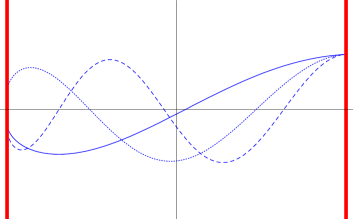
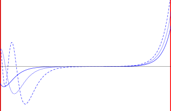
Figure 1: A plot of the first three KK modes for $\alpha=0.01$, we have taken the branes (shown in red) to be at $\pm y_{0}=\pm 33/2$. The masses of the KK modes are given in the final line of Table 1. On the right, for comparison, are the first three eigenfunctions for the RS model.

Like the RS scenario, the behaviour of the massive KK tower is determined by Bessel functions, although in this case they are fractional Bessel functions. Figure 1 shows the first three eigenfunctions, and for comparison the corresponding RS profile. The heterotic eigenfunctions have a much more regular profile along the $y$ direction, which is largely due to the power law, rather than exponential, dependence of the warp factor on $y$.

Drawing this information together, the Green’s function for the spin 2 part of the perturbation on the heterotic braneworld is given in the continuum limit by:

$$G_{R}(x,x^{\prime})=\frac{4\alpha a^{2}(z)a^{2}(z^{\prime})}{a^{8}_{+}}D_{0}(x-x^{\prime})+\int_{0}^{\infty}dm\ u_{m}(z)u_{m}(z^{\prime})D_{m}(x-x^{\prime})$$ (24)

This now allows us to compute the effect in the (positive tension) brane of a source on the brane

$$T^{+}_{ab}=\delta(y-y_{0})T^{+}_{\mu\nu}(x^{\mu})\delta^{\mu}_{a}\delta^{\nu}_{b}$$ (25)

The presence of a source on the brane will in general require the introduction of a nonzero scalar perturbation, and once again we need two coordinate patches, one for each brane. This is a well known result from RS braneworlds, and is interpreted as the brane bending in response to the matter source [26].

The general perturbation has the form:

$$h^{+}_{\mu\nu} = h^{{\tt TT}}_{\mu\nu}+\frac{a^{6}}{2\alpha}F^{+}_{,\mu\nu}+\frac{2\alpha}{a^{4}}F^{+}\eta_{\mu\nu}$$ (26)

$$\delta\phi^{+} = \frac{6\alpha}{a^{6}}F^{+}$$ (27)

where $F^{+}$ is the brane bending term in the coordinate patch of the ‘+’ brane, and is given by:

$$\partial^{2}F^{+}=\kappa_{5}^{2}\frac{T^{+}}{6}$$ (28)

Pulling all the information together, we see that the metric in the brane produced by matter on the brane is, up to a gauge transformation:

$$h^{+}_{\mu\nu}= - 8\alpha\kappa_{5}^{2}\int d^{4}x^{\prime}\;D_{0}(x-x^{\prime})\left[T^{+}_{\mu\nu}-\frac{3}{8}T^{+}\eta_{\mu\nu}\right]$$ (29)

$$- \kappa_{5}^{2}\int d^{4}x^{\prime}\int dm\;u^{2}_{m}(y_{0})D_{m}(x-x^{\prime})\left[T^{+}_{\mu\nu}-\frac{T^{+}}{3}\eta_{\mu\nu}\right]$$

where

$$u_{m}^{2}(y_{0})=\frac{m}{5\alpha}\;\frac{\left[J_{4/5}(\frac{m}{5\alpha})J_{1/5}(\frac{m}{5\alpha})+J_{-4/5}(\frac{m}{5\alpha})J_{-1/5}(\frac{m}{5\alpha})\right]^{2}}{\left[J_{4/5}^{2}(\frac{m}{5\alpha})+J_{-4/5}^{2}(\frac{m}{5\alpha})\right]}$$ (30)

and the dilaton is given by:

$$\delta\phi^{+}=\alpha\kappa^{2}_{5}\int d^{4}x^{\prime}\;D_{0}(x-x^{\prime})\;T^{+}$$ (31)

Thus the brane gravity is a Brans-Dicke theory with $\omega=1/2$.

We now explore the possibilities for a heterotic brane black hole. While we do not have a complete answer to this problem, there are several approaches using both perturbation theory, as well as exact solutions. We start by constructing the black string, and exploring its régime of stability. Continuing the theme of linearized theory, we compare this with the leading order solution for a point particle on the brane. Then we turn to exact approaches, first discussing the possibility of trajectories in known bulks before looking at the full axisymmetric problem and presenting a possible (singular) solution.

3 The Black String and Perturbation Theory

A natural first step in looking for a brane black hole solution is to construct the black string:

$$ds^{2}=a^{2}\left[\left(1-2\frac{G_{N}M}{r}\right)dt^{2}-\left(1-2\frac{G_{N}M}{r}\right)^{-1}dr^{2}-r^{2}d\Omega^{2}_{I\!I}\right]-dy^{2}$$ (32)

However, based on our intuition of cylindrical types of horizon, we expect this black string to be unstable [27]. The instability of the black string in KK theory occurs because there is an unstable massive tensor mode of the 4D Schwarzschild metric, therefore, provided a the perturbations of a spacetime allow a separation of the perturbation into an effective 4D tensor mode with an orthogonal mass eigenfunction, the instability of the string persists to more complicated spacetimes.

It is not difficult to compute the perturbation equations around the curved 4D background, and as in [19] we obtain for the 4D TTF mode:

$$a^{-2}\left(\Box^{(4)}h_{\mu\nu}+2R^{(4)}_{\mu\lambda\nu\rho}h^{\lambda\rho}\right)-h^{\prime\prime}_{\mu\nu}+2\left(\frac{a^{\prime\prime}}{a}+\left(\frac{a^{\prime}}{a}\right)^{2}\right)h_{\mu\nu}=0$$ (33)

where $a(y)$ takes the appropriate form for the heterotic background (5). As this is a tensor mode the scalar perturbations are not excited, at least to linear order. Thus, we can read off the unstable tensor mode as

$$u_{m}(y)h^{(GL)}_{\mu\nu}(t,r)$$ (34)

where $h^{(GL)}_{\mu\nu}(t,r)$ is the unstable mode:

$$h^{(GL)}_{\mu\nu}=e^{\Omega t}\left[\begin{matrix}h_{0}&h_{1}&0&0\cr h_{1}&h_{2}&0&0\cr 0&0&K&0\cr 0&0&0&K\sin^{2}\theta\end{matrix}\right]$$ (35)

and $h_{0},h_{1},h_{2}$ and $K$ are all related via the TTF gauge conditions, and are given in [27]. The parameter $\Omega$ depends on the mass $m$ of the longitudinal tensor $s$-wave, and is found numerically [27], however, for the 4D Schwarzschild metric it is well approximated by:

$$\Omega(m)=\frac{m}{2}-m^{2}G_{N}M\;.$$ (36)

Clearly there will be an unstable mode if the mass of the black string is (roughly) less than $1/2G_{N}m_{0}$, where $m_{0}$ is the minimum eigenvalue permitted for the massive tensor tower. This minimum value depends on $y_{0}$ and $\alpha$, but for $y_{0}\sim 1/6\alpha$, i.e. if the branes are close to their maximal separation, the value is well approximated by $m_{0}\simeq 10\alpha$. Thus the onset of the instability is given by

$$G_{N}M\leq\frac{1}{20\alpha}$$ (37)

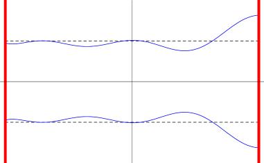
Figure 2: The evolution of the black string instability for the nearly marginal case of $G_{N}M=1$, $\alpha=0.01$, $y_{0}=99/6$. Here only 5 eigenfunctions are below the critical mass value, and the evolution of the event horizon is exaggerated for clarity. The unperturbed event horizon is shown as a dotted black line.

Once the instability has set in, the evolution is similar to the KK string and is shown in figure 2. As with the RS braneworld, the instability is focussed on the brane itself, however, in this case the ripples in the event horizon across the bulk are more uniform, mirroring the behaviour of the transverse eigenfunctions. This does not give any reliable indication of the nonperturbative behaviour, however it is reassuring that the instability does cluster near the brane, rather than having some strong bulk behaviour. One might therefore expect that the true black hole solution would be localized near the brane.

One can also use linearized theory to obtain a far-field approximation of the black hole metric, by computing the linearized solution for a point source on the brane

$$T_{\mu\nu}=M\delta({\bf r})\delta(y-y_{0})\delta_{\mu}^{0}\delta_{\nu}^{0}$$ (38)

For the scalar, (31) immediately gives

$$\phi(r)=\frac{2\alpha G_{5}M}{r}$$ (39)

on the brane. For the tensor, using (29), and expanding the Bessel functions in $u_{m}(0)$ at small $m$ gives a Newtonian potential of

$$V(r)=-\frac{10\alpha G_{5}M}{r}\left(1+\frac{2^{7/5}\Gamma[\frac{8}{5}]}{(5\alpha r)^{8/5}3\Gamma[\frac{4}{5}]^{2}}\right)$$ (40)

This is quite an unusual potential because of the presence of the fractional powers of $r$. Note that it was obtained using the continuum approximation and therefore is only really valid for very small values of $\alpha$, and large values of $y_{0}$.

4 General axisymmetric bulk and the black hole solution

Turning from perturbation theory, a natural approach towards constructing a brane black hole is to use a known bulk and explore possible brane trajectories. Normally, one uses a spherically symmetric bulk, taking the brane trajectory through the bulk at some nontrivial trajectory $\theta(r)$, thereby giving rise to a spherically symmetric brane. Typically, although these trajectories exist, they do not correspond to ‘empty’ branes, and energy momentum is required on the brane to source the gravitational field. These trajectories are solutions of the brane Tolman-Oppenheimer-Volkoff equations (in the context of the RS model, see [28] for work on brane stars and TOV, and [29] for brane and bulk solutions).

Unfortunately, with the bulk action given by (1), there are no spherically symmetric black hole solutions which are asymptotically flat or (a)dS [30]. Indeed, even if one asks for only planar symmetric solutions, the system of Einstein equations has lost its simplicity, and only limited analytic information can be extracted [15]. Spherically symmetric geometries exist only for special values of $\alpha^{2}$, and have unusual asymptotics [31]. In the case of the heterotic braneworld, the sign of the Liouville potential does not permit such a solution, as can be readily seen by attempting to solve (2). It may seem strange that there is no black hole solution, since the geometry has arisen from a compactification from 11 dimensions. However, the wrapped 5 branes, which give rise to the Liouville potential, mean that the dilaton cannot remain fixed in the bulk, and not only remove the possibility of an asymptotically flat solution, but imply an anisotropy in any bulk solution.

It seems therefore that to find a solution, a genuinely axisymmetric bulk metric is required. Using coordinate freedom, this metric can be expressed (up to a 2D conformal gauge group) as [16]:

$$ds^{2}=e^{2\sigma(r,z)}dt^{2}-e^{2\chi(r,z)-\sigma(r,z)}B(r,z)^{-1/2}(dr^{2}+dz^{2})-B(r,z)e^{-\sigma(r,z)}d\Omega^{2}_{I\!I}$$ (41)

This metric has the Einstein equations:

$$\Delta B = \left[2e^{2\chi}-6\alpha^{2}Be^{2\chi-2\phi-\sigma}\right]B^{-1/2}$$ (42)

$$\Delta\sigma+\nabla\sigma\cdot\frac{\nabla B}{B} = -2\alpha^{2}e^{2\chi-2\phi-\sigma}B^{-1/2}$$ (43)

$$\Delta\chi+\frac{3}{4}(\nabla\sigma)^{2}+\frac{1}{4}(\nabla\phi)^{2} = -\frac{e^{2\chi}B^{-3/2}}{2}-\frac{3\alpha^{2}}{2}e^{2\chi-2\phi-\sigma}B^{-1/2}$$ (44)

$$\frac{\partial^{2}_{\pm}B}{B}+\frac{3}{2}(\partial_{\pm}\sigma)^{2}+\frac{1}{2}(\partial_{\pm}\phi)^{2}-2\partial_{\pm}\chi\frac{\partial_{\pm}B}{B} = 0$$ (45)

and for the dilaton:

$$\Delta\phi+\nabla\phi\cdot\frac{\nabla B}{B}=-12\alpha^{2}e^{2\chi-2\phi-\sigma}B^{-1/2}$$ (46)

where $\Delta$ is the 2D Laplacian on $(r,z)$ space, with $\nabla$ as the 2D gradient, and $\partial_{\pm}=\partial_{r}\pm i\partial_{z}$.

This system is similar to the axisymmetric spacetimes explored in [16], where the general axisymmetric Einstein equations were derived, then analyzed in detail for the case of either spherical symmetry, or a cosmological constant. In each case three classes of analytic solution were found. It was noted however, that these were specialized solutions, derived assuming some (albeit minimal) metric Ansatz, and did not represent the full range of possibilities for the spacetime.

In this heterotic case, with both spherical symmetry and the bulk scalar field, the set of equations is more involved, and like the Einstein axisymmetric problem, does not have a general solution generating method. Interestingly however, a simple (and commonly used) Ansatz of separation of metric variables gives just one family of solutions. Setting

$$B = b_{1}(r)b_{2}(z)$$ (47)

$$\sigma = \sigma_{0}+\sigma_{1}(r)+\sigma_{2}(z)$$ (48)

$$\chi = \chi_{0}+\chi_{1}(r)+\chi_{2}(z)$$ (49)

$$\phi = \phi_{0}+\phi_{1}(r)+\phi_{2}(z)$$ (50)

and inspecting (42) suggests that $e^{2\chi}B^{-1/2}$ is a function of $r$, and $e^{2\chi-2\phi-\sigma}B^{-1/2}$ is a function of $z$. Other possibilities are that the roles of $r$ and $z$ are swapped (which would result in a rotation of the branes), or both are a function of $r$ (or $z$). Since it is the first option which corresponds to the LOSW vacuum, we will use this in order to obtain asymptotically flat braneworld solutions.

Using the restrictions on $\chi$ corresponding to $e^{2\chi}B^{-1/2}$ being a function of $r$, and $e^{2\chi-2\phi-\sigma}B^{-1/2}$ a function of $z$, the equations of motion give the following expressions:

$$B = f(z)/g^{\prime}(r)$$ (51)

$$\sigma = \sigma_{0}+ag(r)+\frac{\ln f(z)}{3}-\frac{bc}{3}\zeta$$ (52)

$$\chi = \chi_{0}+\frac{(2b+1)a}{2}g(r)-\frac{1}{4}\ln g^{\prime}(r)+\frac{3}{4}\ln f(z)$$ (53)

$$\phi = \phi_{0}+abg(r)+2\ln f(z)+c\zeta$$ (54)

where $a$, $b$, and $c$ are arbitrary constants, and

$$\zeta=\int\frac{dz}{f}\;.$$ (55)

The Einstein equations give a pair of NLDE’s for $f$ and $g$:

$$\frac{\ddot{f}}{f} = -\frac{2{\dot{f}}^{2}}{3f^{2}}+\left(\frac{b}{3}-2\right)c\frac{\dot{f}}{f^{2}}-\frac{(b^{2}+3)c^{2}}{6f^{2}}=6\alpha^{2}f^{-10/3}e^{-(2-b/3)c\zeta}$$ (56)

$$\left(\frac{1}{g^{\prime}}\right)^{\prime\prime} = \frac{g^{\prime}}{2}\left(\frac{1}{g^{\prime}}\right)^{\prime 2}+(2b+1)ag^{\prime}\left(\frac{1}{g^{\prime}}\right)^{\prime}-\frac{(3+b^{2})a^{2}}{2}g^{\prime}=2e^{2\chi_{0}}\ e^{(2b+1)ag}$$ (57)

where a dot denotes $d/dz$ and a prime $d/dr$. The $f$ equation has the solution

$$f=\left[\frac{2\alpha}{c\beta}\sinh(c\beta\zeta)e^{(b-6)c\zeta/6}\right]^{3/2}$$ (58)

where $\beta^{2}=\frac{2}{3}(1-\frac{b}{2}-\frac{b^{2}}{8})$. The $g$ equation can be integrated by making a change of variable:

$$\rho=\int e^{(2b+1)ag}$$ (59)

which gives

$$g(r)=\frac{1}{2E}\ln\left[\frac{\rho-2E}{\rho}\right]=\frac{1}{2E}\ln V_{s}(\rho)$$ (60)

where $E^{2}=a^{2}(1+b+5b^{2}/4)$, and $V_{s}$ is of course the standard 4D Schwarzschild potential.

Pulling this information together, we see that the general bulk separable solution is:

$$ds^{2} = f^{\frac{2}{3}}e^{\frac{bc\zeta}{3}}\left[V_{s}(\rho)^{\frac{a}{E}}e^{-bc\zeta}dt^{2}-V_{s}(\rho)^{-\frac{(1+b)a}{E}}[d\rho^{2}+\rho(\rho-2E)d\Omega^{2}]-f^{2}V_{s}(\rho)^{\frac{ab}{E}}d\zeta^{2}\right]$$

$$e^{2\phi} = V_{s}(\rho)^{\frac{ab}{E}}f^{4}e^{2c\zeta}$$ (61)

The LOSW vacuum corresponds to $a=c=0$. In this case $E=0$ and all the nontrivial $\rho$-dependence drops out leaving us with

$$ds^{2}=2\alpha\zeta\eta_{\mu\nu}dx^{\mu}dx^{\nu}-(2\alpha\zeta)^{4}d\zeta^{2}$$ (62)

setting $6\alpha y=(2\alpha\zeta)^{3}-1$ recovers the original GN form.

Taking $b=c=0$, but $a=E\neq 0$ recovers the “uniform black string” solution. For $b\neq 0$ however, $a$ is no longer equal to $E$, and the metric and scalar react to the “source”, leading to the metric

$$ds^{2}=a^{2}(y)\left[\left(1-\frac{2E}{\rho}\right)^{\frac{a}{E}}dt^{2}-\left(1-\frac{2E}{\rho}\right)^{-\frac{a(1+b)}{E}}[d\rho^{2}+\rho(\rho-2E)d\Omega^{2}]\right]-\left(1-\frac{2E}{\rho}\right)^{\frac{ab}{E}}dy^{2}$$ (63)

with the scalar given by:

$$e^{2\phi}=\left(1-\frac{2E}{\rho}\right)^{\frac{ab}{E}}a^{12}(y)$$ (64)

The $y$ co-ordinate is no longer a GN coordinate because of the variation of $g_{yy}$ in $\rho$.

Turning to a braneworld solution, we introduce branes at $\zeta=\zeta_{\pm}$, and compute the extrinsic curvature in order to evaluate the boundary conditions:

$$K_{tt} = -f^{2/3}e^{(b-6)c\zeta_{\pm}/3}e^{-\phi}\left(\frac{f_{,\zeta}}{3f}-\frac{ac}{3}\right)g_{tt}$$ (65)

$$K_{\rho\rho} = -f^{2/3}e^{(b-6)c\zeta_{\pm}/3}e^{-\phi}\left(\frac{f_{,\zeta}}{3f}+\frac{ac}{6}\right)g_{\rho\rho}$$ (66)

$$K_{\theta\theta} = -f^{2/3}e^{(b-6)c\zeta_{\pm}/3}e^{-\phi}\left(\frac{f_{,\zeta}}{3f}+\frac{ac}{6}\right)g_{\theta\theta}$$ (67)

Clearly, for a brane solution (energy = tension) we require $ac=0$. The Israel equations then give

$$3\alpha[\cosh(c\beta\zeta)-\beta^{-1}\sinh(c\beta\zeta)]=3\alpha$$ (68)

at either brane. (The sign of the energy term is taken care of by a flip in the sign of the extrinsic curvature due to the normal pointing outwards rather than inwards.) Obviously if $c=0$ this is trivially satisfied, but if instead $a=0$, there is only one solution to (68), $\zeta=0$, hence it is not possible to have the two brane heterotic set-up.

Therefore we conclude that for the two brane spacetime, we require the bulk solution with $c=0$, and so the full spacetime is given by (63), the scalar field by (64), and the branes can be set at any fixed $y$-coordinate, which we will once more take as $y=\pm y_{0}$ to compare with the background LOSW vacuum. Restricting to the $+$ brane, the braneworld solution is

$$ds^{2} = \left(1-\frac{2E}{\rho}\right)^{\frac{a}{E}}dt^{2}-\left(1-\frac{2E}{\rho}\right)^{-\frac{a(1+b)}{E}}[d\rho^{2}+\rho(\rho-2E)d\Omega^{2}]$$ (69)

$$e^{2\phi} = \left(1-\frac{2E}{\rho}\right)^{\frac{ab}{E}}$$ (70)

Note however that the interbrane distance is not a constant:

$$D=\int_{-y_{0}}^{y_{0}}dy|g_{yy}|^{1/2}=2y_{0}V_{s}(\rho)^{\frac{ab}{2E}}$$ (71)

For $ab>0$, the interbrane distance decreases as $\rho$ decreases, eventually closing off the extra dimension at $\rho=2E$. For $ab<0$ however, the reverse is true, the branes move apart until at $\rho=2E$ the transverse separation is infinite.

Figure 3: A plot of the contours of $g_{tt}$ for the singular black tube solution ($\alpha=E=1$). Note that far from the ‘horizon’ the contours become vertical, i.e. depend on the bulk transverse distance, but as $\rho$ decreases, the effect of the source begins to be felt.

Although either option yields a legitimate spherically symmetric braneworld solution, a reasonable approach is to compare this exact solution with the linearized result of the previous section:

$$\delta\phi^{+}=\frac{2\alpha G_{5}M}{r}\qquad h^{+}_{tt}=-\frac{10\alpha G_{5}M}{r}$$ (72)

Expanding (70) at large $\rho$ yields:

$$\phi\simeq-\frac{ab}{\rho}\qquad g_{tt}\simeq 1-\frac{2a}{\rho}$$ (73)

giving:

$$a=5\alpha G_{5}M\qquad b=-2/5$$ (74)

Thus, matching to this linearized solution leads to a bulk in which the branes become infinitely far apart as the null singularity is approached.

Thus, allowing for an axisymmetric bulk with two branes bounding it, and assuming that the metric is separable, we have derived the general brane radially symmetric solution which asymptotes the LOSW vacuum. Unfortunately this solution is singular at $\rho=2E$, however, it does look like the Schwarzschild solution at large $\rho$. The solution very much resembles a string solution, however, the presence of the Schwarzschild potential premultiplying the bulk $z$ coordinate causes the interbrane distance to vary with $\rho$, and in fact the “string” becomes infinite as it becomes singular.

5 Discussion

To sum up, we have explored the existence of braneworld black holes in the heterotic braneworld scenario of Lukas, Ovrut, Stelle and Waldram. We have shown how black string solutions are unstable, and that the linearized solution has rather unusual asymptotics. Unfortunately it was not possible to construct approximate brane stars, as the anisotropic nature of the LOSW vacuum means we have no spherically symmetric bulk black hole solutions. However, we were able to construct an axisymmetric bulk solution which looks like Schwarzschild at large distances, but which is singular as the Schwarzschild radius is approached.

Interestingly, the lack of a spherically symmetric solution for any value of mass means that unlike the RS and ADD models, we are unable to construct even a small black hole perturbatively on the brane (such as the solutions considered in [32]) which seems somehow paradoxical as one might expect a small black hole to be a small perturbation. However, this is really a signal of the different bulk physics. In ADD and RS, the bulk is pure Einstein gravity (with or without a cosmological constant) and at smaller scales the brane becomes less and less relevant. In LOSW however, even a small perturbation will interact with the scalar field, which is the breathing mode of the underlying Calabi-Yau manifold, and thus accesses the higher dimensional physics this indicates.

The existence of these separable axisymmetric solutions is an interesting consequence of the scalar field in the bulk, for the RS model does not have an equivalent solution. The appearance of the Schwarzschild potential to an irrational power is reminiscent of the Poincare invariant $p$-brane solutions in pure gravity [33]. In that case, a string solution in higher dimensions was found, and while the solution was dependent on only one variable (the radial distance) the effect of extra dimensions was to introduce these irrational powers of the Schwarzschild potential. Here we were looking for an axi-symmetric solution, with a warped braneworld interpretation, yet, the effect of the extra dimension turns out to be extremely similar.

The solution which corresponds to the braneworld linearized field at large $\rho$ has the branes diverging as we move in to smaller $\rho$. This is an extremely singular configuration with an infinite bulk null singularity. If however, we relax our requirements and do not demand agreement with the linearized solution, then we can take $b>0$, in which case the bulk pinches off at $\rho=2E$, which is perhaps slightly preferable behaviour. Examining the linearized scalar equation, (31), shows that for the branes to move together, rather than apart, at the linearized level we require $T<0$, in other words, $M<3p$. This would mean matter with a stiff equation of state, and unfortunately does not seem to match the separable solution.

Obviously the ansatz of separability was a choice, used in order to get an exact analytic solution, and may be considered to be too restrictive (although it is a common ansatz used in finding supergravity solutions). Indeed, looking at the behaviour of the linearized solution across the bulk does not appear to give the same dependence as the separable solution, although these are in different gauges. Clearly a numerical integration would give a better indication of the true nature of the solution. However, in spite of all the unattractive features, it is still interesting that the heterotic braneworld does admit an analytic “brane-vacuum” spherically symmetric solution, which is the first example of an exact braneworld ‘black hole’ solution with a consistent bulk in 5 dimensions.

References

-
[1]
V. A. Rubakov,
Phys. Usp. 44, 871 (2001)
[Usp. Fiz. Nauk 171, 913 (2001)]
[arXiv:hep-ph/0104152].
D. Langlois, Prog. Theor. Phys. Suppl. 148, 181 (2003) [arXiv:hep-th/0209261].
P. Brax and C. van de Bruck, Class. Quant. Grav. 20, R201 (2003) [arXiv:hep-th/0303095].
R. Maartens, Living Rev. Rel. 7, 7 (2004) [arXiv:gr-qc/0312059].
S. H. Henry Tye, Lect. Notes Phys. 737, 949 (2008) [arXiv:hep-th/0610221]. -
[2]
N. Arkani-Hamed, S. Dimopoulos and G. R. Dvali,
Phys. Lett. B 429, 263 (1998)
[arXiv:hep-ph/9803315].
I. Antoniadis, N. Arkani-Hamed, S. Dimopoulos and G. R. Dvali, Phys. Lett. B 436, 257 (1998) [arXiv:hep-ph/9804398]. -
[3]
L. Randall and R. Sundrum,
Phys. Rev. Lett. 83, 3370 (1999)
[arXiv:hep-ph/9905221].
L. Randall and R. Sundrum, Phys. Rev. Lett. 83, 4690 (1999) [arXiv:hep-th/9906064]. - [4] S. Kachru, R. Kallosh, A. Linde and S. P. Trivedi, Phys. Rev. D 68, 046005 (2003) [arXiv:hep-th/0301240].
- [5] A. Lukas, B. A. Ovrut, K. S. Stelle and D. Waldram, Phys. Rev. D 59, 086001 (1999) [arXiv:hep-th/9803235].
- [6] J. Khoury, B. A. Ovrut, P. J. Steinhardt and N. Turok, Phys. Rev. D 64, 123522 (2001) [arXiv:hep-th/0103239].
- [7] P. J. Steinhardt and N. Turok, Phys. Rev. D 65, 126003 (2002) [arXiv:hep-th/0111098].
-
[8]
R. Kallosh, L. Kofman and A. D. Linde,
Phys. Rev. D 64, 123523 (2001)
[arXiv:hep-th/0104073].
D. H. Lyth, Phys. Lett. B 524, 1 (2002) [arXiv:hep-ph/0106153].
R. Brandenberger and F. Finelli, JHEP 0111, 056 (2001) [arXiv:hep-th/0109004]. - [9] P. Horava and E. Witten, Nucl. Phys. B 460 (1996) 506 [arXiv:hep-th/9510209]. Nucl. Phys. B 475 (1996) 94 [arXiv:hep-th/9603142].
-
[10]
E. Witten,
Nucl. Phys. B 471, 135 (1996)
[arXiv:hep-th/9602070].
T. Banks and M. Dine, Nucl. Phys. B 479, 173 (1996) [arXiv:hep-th/9605136].
A. Lukas, B. A. Ovrut and D. Waldram, Nucl. Phys. B 532, 43 (1998) [arXiv:hep-th/9710208]. -
[11]
H. A. Chamblin and H. S. Reall,
Nucl. Phys. B 562, 133 (1999)
[arXiv:hep-th/9903225].
P. Binetruy, C. Deffayet and D. Langlois, Nucl. Phys. B 565, 269 (2000) [arXiv:hep-th/9905012].
C. Csaki, M. Graesser, C. F. Kolda and J. Terning, Phys. Lett. B 462, 34 (1999) [arXiv:hep-ph/9906513].
J. M. Cline, C. Grojean and G. Servant, Phys. Rev. Lett. 83, 4245 (1999) [arXiv:hep-ph/9906523].
P. Kraus, JHEP 9912, 011 (1999) [arXiv:hep-th/9910149].
P. Binetruy, C. Deffayet, U. Ellwanger and D. Langlois, Phys. Lett. B 477, 285 (2000) [arXiv:hep-th/9910219]. - [12] P. Bowcock, C. Charmousis and R. Gregory, Class. Quant. Grav. 17, 4745 (2000) [arXiv:hep-th/0007177].
-
[13]
A. Lukas, B. A. Ovrut and D. Waldram,
Phys. Rev. D 60, 086001 (1999)
[arXiv:hep-th/9806022].
H. S. Reall, Phys. Rev. D 59, 103506 (1999) [arXiv:hep-th/9809195].
A. Lukas, B. A. Ovrut and D. Waldram, Phys. Rev. D 61, 023506 (2000) [arXiv:hep-th/9902071].
U. Ellwanger, Eur. Phys. J. C 25, 157 (2002) [arXiv:hep-th/0001126].
R. L. Arnowitt, J. Dent and B. Dutta, Phys. Rev. D 70, 126001 (2004) [arXiv:hep-th/0405050]. -
[14]
J. L. Lehners, P. McFadden and N. Turok,
Phys. Rev. D 75, 103510 (2007)
[arXiv:hep-th/0611259].
P. McFadden, arXiv:hep-th/0612008.
J. L. Lehners, P. McFadden and N. Turok, Phys. Rev. D 76, 023501 (2007) [arXiv:hep-th/0612026]. - [15] C. Charmousis, Class. Quant. Grav. 19, 83 (2002) [arXiv:hep-th/0107126].
- [16] C. Charmousis and R. Gregory, Class. Quant. Grav. 21, 527 (2004) [arXiv:gr-qc/0306069].
- [17] R. Gregory, “Braneworld black holes,” arXiv:0804.2595 [hep-th].
- [18] A. Chamblin, S. W. Hawking and H. S. Reall, Phys. Rev. D 61 (2000) 065007 [arXiv:hep-th/9909205].
- [19] R. Gregory, Class. Quant. Grav. 17, L125 (2000) [arXiv:hep-th/0004101].
-
[20]
H. L. Verlinde,
Nucl. Phys. B 580, 264 (2000)
[arXiv:hep-th/9906182].
S. S. Gubser, Phys. Rev. D 63, 084017 (2001) [arXiv:hep-th/9912001].
E. P. Verlinde and H. L. Verlinde, JHEP 0005, 034 (2000) [arXiv:hep-th/9912018]. M. J. Duff and J. T. Liu, Phys. Rev. Lett. 85, 2052 (2000) [Class. Quant. Grav. 18, 3207 (2001)] [arXiv:hep-th/0003237]. -
[21]
T. Tanaka,
Prog. Theor. Phys. Suppl. 148, 307 (2003)
[arXiv:gr-qc/0203082].
R. Emparan, A. Fabbri and N. Kaloper, JHEP 0208, 043 (2002) [arXiv:hep-th/0206155]. -
[22]
A. L. Fitzpatrick, L. Randall, and T. Wiseman,
JHEP 0611, 033 (2006)
hep-th/0608208.
A. Fabbri and G. P. Procopio, Class. Quant. Grav. 24, 5371 (2007), 0704.3728 [hep-th].
A. Fabbri and G. P. Procopio, “The Holographic Interpretation of Hawking Radiation,” arXiv:0705.3363 [gr-qc].
T. Tanaka, “Implication of Classical Black Hole Evaporation Conjecture to Floating Black Holes,” arXiv:0709.3674 [gr-qc].
L. Grisa and O. Pujolas, JHEP 0806, 059 (2008) [arXiv:0712.2786 [hep-th]].
R. Gregory, S. F. Ross and R. Zegers, JHEP 0809, 029 (2008) [arXiv:0802.2037 [hep-th]].
A. Flachi and T. Tanaka, “Vacuum polarization in asymptotically anti-de Sitter black hole geometries,” arXiv:0803.3125 [hep-th].
O. Pujolas, “Strongly Coupled Radiation from Moving Mirrors and Holography in the Karch-Randall model,” arXiv:0809.0005 [hep-th].
H. Yoshino, “On the existence of a static black hole on a brane,” arXiv:0812.0465 [gr-qc]. - [23] C. Charmousis, R. Gregory and V. A. Rubakov, Phys. Rev. D 62, 067505 (2000) [arXiv:hep-th/9912160].
- [24] O. Seto and H. Kodama, Phys. Rev. D 63, 123506 (2001) [arXiv:hep-th/0012102].
-
[25]
P. Brax and A. C. Davis,
Phys. Lett. B 497, 289 (2001)
[arXiv:hep-th/0011045].
G. Cynolter, Mod. Phys. Lett. A 20 (2005) 519 [arXiv:hep-th/0209152].
P. Brax, C. van de Bruck, A. C. Davis and C. S. Rhodes, Phys. Lett. B 531 (2002) 135 [arXiv:hep-th/0201191]. - [26] J. Garriga and T. Tanaka, Phys. Rev. Lett. 84, 2778 (2000) [arXiv:hep-th/9911055].
-
[27]
R. Gregory and R. Laflamme,
Phys. Rev. Lett. 70, 2837 (1993)
[arXiv:hep-th/9301052].
R. Gregory and R. Laflamme, Nucl. Phys. B 428, 399 (1994) [arXiv:hep-th/9404071]. -
[28]
N. Dadhich, R. Maartens, P. Papadopoulos and V. Rezania,
Phys. Lett. B 487, 1 (2000)
[arXiv:hep-th/0003061].
C. Germani and R. Maartens, Phys. Rev. D 64, 124010 (2001) [arXiv:hep-th/0107011].
G. Kofinas, E. Papantonopoulos and I. Pappa, Phys. Rev. D 66, 104014 (2002) [arXiv:hep-th/0112019].
J. Ovalle, “Non-uniform Braneworld Stars: an Exact Solution,” arXiv:0809.3547 [gr-qc]. -
[29]
S. S. Seahra,
Phys. Rev. D 71, 084020 (2005)
[arXiv:gr-qc/0501018].
C. Galfard, C. Germani and A. Ishibashi, Phys. Rev. D 73, 064014 (2006) [arXiv:hep-th/0512001].
S. Creek, R. Gregory, P. Kanti and B. Mistry, Class. Quant. Grav. 23, 6633 (2006) [arXiv:hep-th/0606006]. - [30] S. J. Poletti and D. L. Wiltshire, Phys. Rev. D 50, 7260 (1994) [Erratum-ibid. D 52, 3753 (1995)] [arXiv:gr-qc/9407021].
- [31] K. C. Chan, J. H. Horne and R. B. Mann, Nucl. Phys. B 447, 441 (1995) [arXiv:gr-qc/9502042].
-
[32]
N. Dadhich, R. Maartens, P. Papadopoulos and V. Rezania,
Phys. Lett. B 487, 1 (2000)
[arXiv:hep-th/0003061].
R. Casadio and B. Harms, Phys. Lett. B 487, 209 (2000) [arXiv:hep-th/0004004].
S. Dimopoulos and G. L. Landsberg, Phys. Rev. Lett. 87, 161602 (2001) [arXiv:hep-ph/0106295].
P. Kanti, “Reading the number of extra dimensions in the spectrum of Hawking radiation,” arXiv:hep-ph/0310162. - [33] R. Gregory, Nucl. Phys. B 467, 159 (1996) [arXiv:hep-th/9510202].