A sample of GHz-peaked spectrum sources selected at RATAN–600: spectral and variability properties

Abstract

We describe a new sample of 226 GPS (GHz-Peaked Spectrum) source candidates selected using simultaneous 1–22 GHz multi-frequency observations with the RATAN–600 radio telescope. Sixty objects in our sample are identified as GPS source candidates for the first time. The candidates were selected on the basis of their broad-band radio spectra only. We discuss the spectral and variability properties of selected objects of different optical classes.

1 Introduction

The first samples of GHz-Peaked Spectrum sources (e.g., Gopal-Krishna, Patnaik & Steppe 1983) were selected solely on the basis of radio spectra properties. Later samples, like the one presented by Snellen et al. (2002) were considering other factors such as optical counterpart type during the selection process. The very meaning of the word “GPS source” has shifted from the description of spectral shape to something close to “probable young radio source” which are believed to be found among sources with convex spectra.

In this work we use the “old fashioned” spectral-only approach to select one of the largest samples of peaked spectrum sources to date. Special care is taken to keep the sample as free as possible from sources which change their overall spectral shape due to variability. We investigate the observed properties of sources from the sample to test the idea that sources with peaked spectra are a mixture of intrinsically different types of AGN (e.g., Stanghellini 2003).

2 Observational data and sample selection

To select GPS source candidates we use 1–22 GHz multi-frequency data from the RATAN–600 telescope of the Special Astrophysical Observatory, Russian Academy of Sciences. It is a 576 m diameter ring radio telescope situated at stanitsa Zelenchukskaya, Karachay-Cherkessia, Russia. The telescope is mostly operated in transit mode. Emission from a radio source is measured as it crosses the feed beams of the broad-band receivers operating at 1, 2.3, 3.9 (or 4.8), 7.7, 11 and 22 GHz. This allows us to obtain the source spectra over a few minutes only. The exact time it takes the source to cross all beams (and hence the integration time) is a function of the source declination. Details of the method used for the observations and data processing can be found in Kovalev et al. (1999).

We use spectra of 4047 sources observed with RATAN from 1997 to 2006 during multifrequency monitoring and survey campaigns conducted by Kovalev et al. (1999, 2000, 2002). The observed source list includes a complete sample of sources with $\delta>-30$ and a total VLBI flux density at 8 GHz greater than 200 mJy (Kovalev et al. 2007). To improve the frequency coverage, we combine our RATAN–600 data with previously published measurements collected by the CATS database (Verkhodanov et al. 2005).

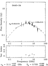
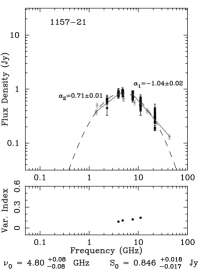
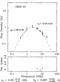
Figure 1: Radio spectra of 3 out of 60 newly identified GPS source candidates. Variability index as a function of frequency is presented in the panels under the spectra plots. Black points correspond to RATAN–600 data, grey points represent data collected from the literature.

Figure 2: Combined spectra of all selected 226 GPS candidates normalized by peak flux density and peak frequency values. Filled circles represent the observed spectra binned and shifted along the vertical axis. The solid line is a normalized and shifted theoretical spectrum of a homogeneous synchrotron emitting cloud with self-absorption and power index $\gamma=2.54$ of electrons energy distribution.

We inspected all of the collected broad-band spectra to select sources which show a prominent spectral peak at all epochs for which we have RATAN data (supplemented by the CATS database). To derive the peak flux density ($S_{\nu_{0}}$) and peak frequency ($\nu_{0}$), we followed O’Dea et al. (1990), Snellen et al. (2002) and Edwards & Tingay (2004), and fitted each source spectrum in the log-log scale with a parabolic function $\log S_{\nu}=a(\log\nu)^{2}+b\log\nu+c$, were $S_{\nu}$ is the flux density at frequency $\nu$, $a$, $b$, and $c$ are coefficients determined using a least square regression method. Despite having no physical meaning, this simple fit can represent observations reasonably well. The spectral indexes were determined by fitting the high- and low-frequency regions of the spectra with a linear function in the log-log scale. We have used similar criteria to those suggested by de Vries, Barthel & O’Dea (1997) to select the final list of GPS candidates: (i) source spectra show a defined peak at a frequency above $500$ MHz, (ii) the difference between the high- and low-frequency spectral indexes is greater than $0.6$. We use the traditional $500$ MHz boundary between GPS and Compact Steep Spectrum (CSS) sources, despite there is no clear physical boundary between them, because we do not have our own observations at frequencies below 1 GHz.

We have selected a sample of 226 GPS source candidates, 60 objects from the sample have never been reported before as GPS source candidates (see examples in Fig. 1). Optical identifications and redshift information were extracted from the Véron-Cetty & Véron (2006) catalog and NED (NASA/IPAC Extragalactic Database). Spectroscopic redshifts were found for 128 sources, 39 sources are identified with galaxies, 98 are identified with quasars, three sources (PKS 0637$-$337, PKS 1300$-$105, and PKS 1519$-$273) are BL Lacertae objects. For 86 sources no optical identification was found (empty fields).

3 Spectral properties

An “average” GPS spectrum in our sample is characterized by the peak frequency $\nu_{0}=2.4$ GHz and flux density $S_{\nu_{0}}=0.8$ Jy. The spectral indexes above and below the turnover frequency are $\alpha_{1}=-0.77$ and $\alpha_{2}=0.66$.

To provide a quick impression of the spectra selected, we present Fig. 2. An average spectrum of a GPS source was constructed by combining the individual source spectra normalized by their peak frequency and flux density. This combined spectrum is compared to a theoretical spectrum of a homogeneous synchrotron emitting cloud with a spectral index above the peak equal to the median value for our sample.

As can be seen from Fig. 2, the observed spectra of GPS sources are wider and do not reach $\alpha_{2}=5/2$ which is predicted by synchrotron self-absorption. In fact, no single source in our sample approaches this value. The most inverted $\alpha_{2}=1.76\pm 0.03$ is found in the known GPS quasar 0457+024. Among the 10 sources with the most inverted spectra there are five quasars, one radio galaxy and four empty fields. The absence of observed $\alpha_{2}\sim 5/2$ means that the radiation of GPS sources can not be described assuming one homogeneous synchrotron self-absorbed cloud. There should be a significant non-homogeneity in the properties across the volume of the radio–emitting region.

The broad-band radio spectra of GPS galaxies and quasars look very much alike. We found no significant differences in the low-frequency spectral index distribution between subgroups of our sample: galaxies, quasars and unidentified radio sources. This may be an indication of a common mechanism responsible for the absorption at low frequencies. The median value of high-frequency spectral index is $\alpha^{\mathrm{gal}}_{1}=-0.80$ for galaxies and $\alpha^{\mathrm{qso}}_{1}=-0.71$ for quasars. The Kolmogorov-Smirnov (KS) test has also confirmed that the distribution for galaxies and quasars are not different significantly.

No difference was found in the observed peak flux density between galaxies and quasars. However, when it comes to the peak frequency distribution (Fig. 3), the KS test shows that there is only a 10 per cent chance that the observed peak frequency distributions of galaxies and quasars are drawn from the same parent distribution. If we consider the peak frequency in the source frame, this probability drops to 0.01 per cent. Galaxies in our sample are characterized by a lower intrinsic peak frequency (median value 3 GHz) than quasars (8.8 GHz). This is expected since quasars are found, in general, at higher redshifts.

Figure 3: Peak frequency distribution for GPS quasars, galaxies and unidentified radio sources (empty fields).

4 Variability

For the 108 sources which have observations with RATAN–600 at three or more epochs, a variability study was carried out. We concentrate on the variability properties at 11 GHz which corresponds to the optically thin part of the synchrotron spectrum for the majority of the sources. In addition, this band is almost RFI free, has high sensitivity and is not affected significantly by weather. Sources with a peak frequency around or above 11 GHz are excluded from the analysis in order to probe variability at a frequency with no self-absorption.

To characterize the variability amplitude of sources we use the variability index (e.g., used by Aller, Aller & Hughes 1992) applying the modified robust form:

$$v=\frac{(S_{i}-\sigma_{i})_{\mathrm{max}}-(S_{i}+\sigma_{i})_{\mathrm{min}}}{(S_{i}-\sigma_{i})_{\mathrm{max}}+(S_{i}+\sigma_{i})_{\mathrm{min}}}\,$$

$S_{i}$ and $\sigma_{i}$ are the source flux density and RMS error measured at $i$’th epoch, max/min indexes correspond to the maximum/minimum value among all epochs. Note, that $v$ can be negative if the estimated error $\sigma$ is greater than the observed scatter of the data. The relative accuracy of flux density measurements as well as the number of observations influences the value of $v$. We have modeled the variability index distribution for a sample of non-variable sources which have fluxes that are measured with a typical accuracy of the RATAN measurements (assuming Gaussian noise). In this modeling we have used the actual distribution of the number of observations. We conclude that sources with $v\geq 0.15$ can be considered as significantly variable.

Figure 4: Distribution of variability index $v_{11}$ at 11 GHz for GPS quasars, galaxies and unidentified radio sources (empty fields) in our sample.

The distribution of $v_{11}$ is found to be different for galaxies and quasars (Fig. 4). There are many variable sources among quasars. The statistics for galaxies is suffering from the small number of objects, but it can be clearly divided into two groups: the main distribution which is consistent with non-variable or weakly variable sources, with variations under 9–10 per cent. The second group consist of three strongly variable galaxies: PKS 0500$+$019, note that this object is listed as a quasar by Becker, White & Edwards (1991); TXS 1404$+$286 (OQ 208, Mkn 668), its variability at a frequency above the peak was first reported by Stanghellini et al. (1997); and B2 1600$+$33.

A KS test gives a 63 per cent probability that galaxies (with the exception of three clearly variable cases) and “empty fields” are drawn from the same distribution of variability index at 11 GHz. The same probability for galaxies and quasars is neglectable ($<0.01$ per cent). This implies that most of the optically unidentified GPS sources might be faint distant galaxies and not quasars. The similarity of the observed peak frequency distribution for galaxies and “empty fields” (Fig. 3) supports this conclusion. This may suggest, that the observed difference in redshift distributions of GPS quasars and galaxies (Fig. 5) can not be used as an argument in support of the idea that these two types of GPS sources are intrinsically different. If there is a large number of distant GPS galaxies which lack an optical identification that are also optically faint, then the difference in the redshift distribution may be attributed to a selection effect.

Figure 5: Redshift distribution of GPS galaxies and GPS quasars from the sample.

5 Summary

We have selected a sample of 226 GPS source candidates from multi-frequency, multi-epoch observations conducted at the RATAN–600 radio telescope, supplemented by the literature; 60 objects from the sample are reported as GPS candidates for the first time.

Derived parameters of the convex spectra do not allow us to distinguish between GPS galaxies and quasars. GPS quasars tend to show significantly stronger variability than GPS galaxies, which is in agreement with previously published results for both GPS (e.g., O’Dea 1998) and high frequency peaked (Tinti et al. 2005) sources. Most GPS galaxies and “empty fields” show no significant variability with three noticeable exceptions: PKS 0500$+$019, TXS 1404$+$28, and B2 1600$+$33. The low variability of GPS sources with no optical identification suggests that a significant fraction of them might be optically faint and, possibly, distant GPS galaxies. GPS galaxies and GPS quasars have significantly different variability properties and intrinsic peak frequencies. However, no clear boundary can be drawn between them on the basis of single-dish radio observations because GPS galaxies and GPS quasars strongly overlap in their observed properties.

We plan to extend our study of the selected GPS sample to parsec scales by analyzing simultaneous 2 and 8 GHz VLBA observations from the VLBA Calibrator survey (Beasley et al. 2002, Fomalont et al. 2003, Petrov et al. 2004, 2005, 2008, Kovalev et al. 2007).

- [1] Aller, M.F., Aller, H.D., Hughes, P.A.: 1992, ApJ 399, 16
- [2] Beasley, A.J., et al.: 2002, ApJS 141, 13
- [3] Becker, R.H., White, R.L., Edwards, A.L.: 1991, ApJS 75, 1
- [4] de Vries, W.H., Barthel, P.D., O’Dea, C.P.: 1997, A&A 321, 105
- [5] Edwards, P.G. and Tingay, S.J.: 2004, A&A 424, 91
- [6] Fomalont, E.B., et al.: 2003, AJ 126, 2562
- [7] Gopal-Krishna, Patnaik, A.R., Steppe, H.: 1983, A&A 123, 107
- [8] Kovalev, Yu.A., Kovalev, Y.Y., & Nizhelsky, N.A.: 2000, PASJ 52, 1027
- [9] Kovalev, Y.Y., et al.: 1999, A&AS 139, 545
- [10] Kovalev, Y.Y., Kovalev, Y.A., Nizhelsky, N.A., Bogdantsov, A.B.: 2002, PASA 19, 83
- [11] Kovalev, Y.Y., Petrov, L., Fomalont, E.B., & Gordon, D.: 2007, AJ 133, 1236
- [12] O’Dea, C.P., Baum, S.A., Stanghellini, C., Morris, G.B., Patnaik, A.R., Gopal-Krishna: 1990, A&AS 84, 549
- [13] O’Dea, C.P., 1998, PASP 110, 493
- [14] Petrov, L., Kovalev, Y.Y., Fomalont, E.B., & Gordon, D.: 2008 AJ 136, 580
- [15] Petrov, L., Kovalev, Y.Y., Fomalont, E.B., & Gordon, D.: 2006, AJ 131, 1872
- [16] Petrov, L., Kovalev, Y.Y., Fomalont, E.B., & Gordon, D.: 2005, AJ 129, 1163
- [17] Snellen, I.A.G., Lehnert, M.D., Bremer, M.N., Schilizzi, R.T.: 2002, MNRAS 337, 981
- [18] Stanghellini, C., Bondi, M., Dallacasa, D., O’Dea, C.P., Baum, S.A., Fanti, R., Fanti, C.: 1997, A&A 318, 376
- [19] Stanghellini, C., O’Dea, C.P., Dallacasa, D., Baum, S.A., Fanti, R., Fanti, C.: 1998, A&AS 131, 303
- [20] Stanghellini, C.: 2003, PASA 20, 118
- [21] Tinti, S., Dallacasa, D., de Zotti, G., Celotti, A., Stanghellini, C.: 2005, A&A 432, 31
- [22] Verkhodanov O.V., Trushkin S.A., Andernach H., & Chernenkov V.N.: 2005, Bull. SAO 58, 118; arXiv:0705.2959
- [23] Véron-Cetty, M.-P. and Véron, P.: 2006, A&A 455, 773