Measuring the tensor to scalar ratio from CMB B-modes in presence of foregrounds

Abstract

Aims. We investigate the impact of polarised foreground emission on the performances of future CMB experiments aiming the detection of primordial tensor fluctuations in the early universe. In particular, we study the accuracy that can be achieved in measuring the tensor–to–scalar ratio $r$ in presence of foregrounds.

Methods. We design a component separation pipeline, based on the Smica method, aimed at estimating $r$ and the foreground contamination from the data with no prior assumption on the frequency dependence or spatial distribution of the foregrounds. We derive error bars accounting for the uncertainty on foreground contribution. We use the current knowledge of galactic and extra-galactic foregrounds as implemented in the Planck Sky Model (PSM), to build simulations of the sky emission. We apply the method to simulated observations of this modelled sky emission, for various experimental setups.

Results. Our method, with Planck data, permits us to detect $r=0.1$ from B-modes only at more than 3$\sigma$. With a future dedicated space experiment, as EPIC, we can measure $r=0.001$ at $\sim 6\sigma$ for the most ambitious mission designs. Most of the sensitivity to $r$ comes from scales $20\leq\ell\leq 150$ for high $r$ values, shifting to lower $\ell$’s for progressively smaller $r$. This shows that large scale foreground emission doesn’t prevent a proper measurement of the reionisation bump for full sky experiment. We also investigate the observation of a small but clean part of the sky. We show that diffuse foregrounds remain a concern for a sensitive ground–based experiment with a limited frequency coverage when measuring $r<0.1$. Using the Planck data as additional frequency channels to constrain the foregrounds in such ground–based observations reduces the error by a factor two but does not allow to detect $r=0.01$. An alternate strategy, based on a deep field space mission with a wide frequency coverage, would allow us to deal with diffuse foregrounds efficiently, but is in return quite sensitive to lensing contamination. In the contrary, we show that all-sky missions are nearly insensitive to small scale contamination (point sources and lensing) if the statistical contribution of such foregrounds can be modelled accurately. Our results do not significantly depend on the overall level and frequency dependence of the diffused foreground model, when varied within the limits allowed by current observations.

1 Introduction

After the success of the WMAP space mission in mapping the Cosmic Microwave Background (CMB) temperature anisotropies, much attention now turns towards the challenge of measuring CMB polarisation, in particular pseudo-scalar polarisation modes (the B-modes) of primordial origin. These B-modes offer one of the best options to constrain inflationary models (1997PhRvL..78.2054S; 1997NewA....2..323H; 1997PhRvL..78.2058K; 1998PhRvD..57..685K; 2008arXiv0810.3022B).

First polarisation measurements have already been obtained by a number of instruments (2002Natur.420..772K; 2005AAS...20710007S; 2007ApJS..170..335P), but no detection of B-modes has been claimed yet. While several ground–based and balloon–borne experiments are already operational, or in construction, no CMB–dedicated space-mission is planned after Planck at the present time: whether there should be one for CMB B-modes, and how it should be designed, are still open questions.

As CMB polarisation anisotropies are expected to be significantly smaller than temperature anisotropies (a few per cent at most), improving detector sensitivities is the first major challenge towards measuring CMB polarisation B-modes. It is not, however, the only one. Foreground emissions from the galactic interstellar medium (ISM) and from extra-galactic objects (galaxies and clusters of galaxies) superimpose to the CMB. Most foregrounds are expected to emit polarised light, with a polarisation fraction typically comparable, or larger, than that of the CMB. Component separation (disentangling CMB emission from all these foregrounds) is needed to extract cosmological information from observed frequency maps. The situation is particularly severe for the B-modes of CMB polarisation, which will be, if measurable, sub-dominant at every scale and every frequency.

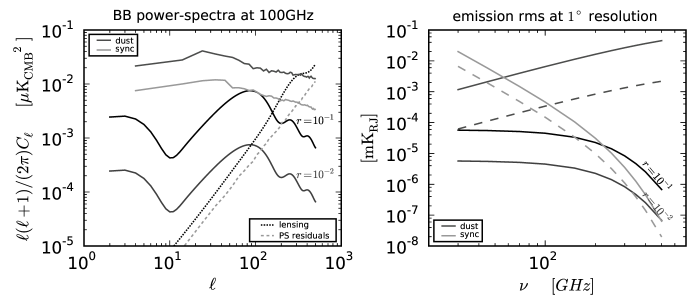
Figure 1: Respective emission levels of the various components as predicted by the PSM. Left: predicted power spectra of the various components at 100 GHz, compared to CMB and lensing level for standard cosmology and various values of $r$ ($\tau=0.07$, and other cosmological parameters follow 2008arXiv0803.0586D). The power spectra of diffuse galactic foregrounds are computed using the cleanest 55% of the polarised sky. The power spectrum from residual point sources is computed assuming that all sources brighter than 500 mJy (in temperature) in one of the Planck channels have been cut out. Right: typical frequency-dependence of the contributions to B-type polarisation of CMB, synchrotron and dust, at 1 degree resolution. The dashed lines correspond to the mean level of fluctuation as computed outside the mask used for the power spectra shown in the right panel.

The main objective of this paper is to evaluate the accuracy with which various upcoming or planned experiments can measure $r$ in presence of foregrounds. This problem has been addressed before: 2005MNRAS.360..935T investigate the lower bound for $r$ that can be achieved considering a simple foreground cleaning technique, based on the extrapolation of foreground templates and subtraction from a channel dedicated to CMB measurement; 2006JCAP...01..019V assume foreground residuals at a known level in a cleaned map, treat them as additional Gaussian noise, and compute the error on $r$ due to such excess noise; 2007PhRvD..75h3508A investigate how best to select the frequency bands of an instrument, and how to distribute a fixed number of detectors among them, to maximally reject galactic foreground contamination. This latter analysis is based on an Internal Linear Combination cleaning technique similar to the one of 2003PhRvD..68l3523T on WMAP temperature anisotropy data. The two last studies assume somehow that the residual contamination level is perfectly known – an information which is used to derive error bars on $r$.

In this paper, we relax this assumption and propose a method to estimate the uncertainty on residual contamination from the data themselves, as would be the case for real data analysis. We test our method on semi-realistic simulated data sets, including CMB and realistic foreground emission, as well as simple instrumental noise. We study a variety of experimental designs and foreground mixtures.

This paper is organised as follows: the next section (Sect. 2) deals with polarised foregrounds and presents the galactic emission model used in this work. In section 3, we propose a method, using the most recent version of the Smica component separation framework (2008arXiv0803.1814C), to provide measurements of the tensor to scalar ratio in presence of foregrounds. In section 4, we present the results obtained by applying the method to various experimental designs. Section LABEL:sec:discussion discusses the reliability of the method (and of our conclusions) against various issues, in particular modelling uncertainty. Main results are summarised in section LABEL:sec:conclusion.

2 Modelling polarised sky emission

Several processes contribute to the total sky emission in the frequency range of interest for CMB observation (typically between 30 and 300 GHz). Foreground emission arises from the galactic interstellar medium (ISM), from extra-galactic objects, and from distortions of the CMB itself through its interaction with structures in the nearby universe. Although the physical processes involved and the general emission mechanisms are mostly understood, specifics of these polarised emissions in the millimetre range remain poorly known as few actual observations, on a significant enough part of the sky, have been made.

Diffuse emission from the ISM arises through synchrotron emission from energetic electrons, through free–free emission, and through grey-body emission of a population of dust grains. Small spinning dust grains with a dipole electric moment may also emit significantly in the radio domain (1998ApJ...508..157D). Among those processes, dust and synchrotron emissions are thought to be significantly polarised. Galactic emission also includes contributions from compact regions such as supernovae remnants and molecular clouds, which have specific emission properties.

Extra-galactic objects emit via a number of different mechanisms, each of them having its own spectral energy distribution and polarisation properties.

Finally, the CMB polarisation spectra are modified by the interactions of the CMB photons on their way from the last scattering surface. Reionisation, in particular, re-injects power in polarisation on large scales by late-time scattering of CMB photons. This produces a distinctive feature, the reionisation bump, in the CMB B-mode spectrum at low $\ell$. Other interactions with the latter universe, and in particular lensing, contribute to hinder the measurement of the primordial signal. The lensing effect is particularly important on smaller scales as it converts a part of the dominant E-mode power into B-mode.

In the following, we review the identified polarisation processes and detail the model used for the present work, with a special emphasis on B-modes. We also discuss main sources of uncertainty in the model, as a basis for evaluating their impact on the conclusions of this paper.

Our simulations are based on the Planck Sky Model (PSM), a sky emission simulation tool developed by the Planck collaboration for pre-launch preparation of Planck data analysis (Delabrouille09). Figure 1 gives an overview of foregrounds as included in our baseline model. Diffuse galactic emission from synchrotron and dust dominates at all frequencies and all scales, with a minimum (relative to CMB) between 60 and 80 GHz, depending on the galactic cut. Contaminations by lensing and a point source background are lower than primordial CMB for $r>0.01$ and for $\ell<100$, but should clearly be taken into account in attempts to measure $r<0.01$.

2.1 Synchrotron

Cosmic ray electrons spiralling in the galactic magnetic field produce highly polarised synchrotron emission (e.g. 1979rpa..book.....R). This is the dominant contaminant of the polarised CMB signal at low frequency ($\lesssim 80\,\text{GHz}$), as can be seen in the right panel of Fig. 1. In the frequency range of interest for CMB observations, measurements of this emission have been provided, both in temperature and polarisation, by WMAP (2007ApJS..170..335P; 2008arXiv0803.0715G). The intensity of the synchrotron emission depends on the cosmic ray density $n_{e}$, and on the strength of the magnetic field perpendicularly to the line of sight. Its frequency scaling and its intrinsic polarisation fraction $f_{s}$ depend on the energy distribution of the cosmic rays.

2.1.1 Synchrotron emission law

For electron density following a power law of index $p$, $n_{e}(E)\varpropto E^{-p}$, the synchrotron frequency dependence is also a power law, of index $\beta_{s}=-(p+3)/2$:

$$S(\nu)=S(\nu_{0})(\nu/\nu_{0})^{\beta_{s}}$$ (1)

where the spectral index, $\beta_{s}$, is equal to $-3$ for a typical value $p=3$.

The synchrotron spectral index depends significantly on cosmic ray properties. It varies with the direction of the sky, and possibly, with the frequency of observation (see e.g. 2007ARNPS..57..285S for a review of propagation and interaction processes of cosmic rays in the galaxy).

For a multi-channel experiment, the consequence of this is a decrease of the coherence of the synchrotron emission across channels, i.e. the correlation between the synchrotron emission in the various frequency bands of observation will be below unity.

Observational constraints have been put on the synchrotron emission law. A template of synchrotron emission intensity at 408 MHz has been provided by 1982A&AS...47....1H. Combining this map with sky surveys at 1.4 GHz (1986A&AS...63..205R) and 2.3 GHz (1998MNRAS.297..977J), 2002A&A...387...82G and 2003A&A...410..847P have derived nearly full sky spectral index maps. Using the measurement from WMAP, 2003ApJS..148...97B derived the spectral index between 408 MHz and 23 GHz. Compared to the former results, it showed a significant steepening toward $\beta_{s}=-3$ around 20 GHz, and a strong galactic plane feature with flatter spectral index. This feature was first interpreted as a flatter cosmic ray distribution in star forming regions. Recently, however, taking into account the presence, at 23 GHz, of additional contribution from a possible anomalous emission correlated with the dust column density, 2008arXiv0802.3345M found no such pronounced galactic feature, in better agreement with lower frequency results. The spectral index map obtained in this way is consistent with $\beta_{s}=-3\pm 0.06$.

There is, hence, still significant uncertainty on the exact variability of the synchrotron spectral index, and in the amplitude of the steepening if any.

2.1.2 Synchrotron polarisation

If the electron density follows a power law of index $p$, the synchrotron polarisation fraction reads:

$$f_{s}=3(p+1)/(3p+7)$$ (2)

For $p=3$, we get $f_{s}=0.75$, a polarisation fraction which varies slowly for small variations of $p$. Consequently, the intrinsic synchrotron polarisation fraction should be close to constant on the sky. However, geometric depolarisation arises due to variations of the polarisation angle along the line of sight, partial cancellation of polarisation occurring for superposition of emission with orthogonal polarisation directions. Current measurements show variations of the observed polarisation value from about 10% near the galactic plane, to 30-50 % at intermediate to high galactic latitudes (Macellari08).

2.1.3 Our model of synchrotron

In summary, the B-mode intensity of the synchrotron emission is modulated by the density of cosmic rays, the slope of their spectra, the intensity of the magnetic field, its orientation, and the coherence of the orientation along the line of sight. This makes the amplitude and frequency scaling of the polarised synchrotron signal dependant on the sky position in a rather complex way.

For the purpose of the present work, we mostly follow 2008arXiv0802.3345M model 4, using the same synchrotron spectral index map, and the synchrotron polarised template at 23 GHz measured by WMAP. This allows the definition of a pixel-dependent geometric depolarisation factor $g(\xi)$, computed as the ratio between the polarisation expected theoretically from Eq. 2, and the polarisation actually observed. This depolarisation, assumed to be due to varying orientations of the galactic magnetic field along the line of sight, is used also for modelling polarised dust emission (see below).

As an additional refinement, we also investigate the impact of a slightly modified frequency dependence with a running spectral index in Sect. LABEL:sec:discussion. For this purpose, the synchrotron emission Stokes parameters ($S_{\nu}^{X}(\xi)$ for $X\in\{Q,U\}$), at frequency $\nu$ and in direction $\xi$ on the sky, will be modelled instead as:

$$S_{\nu}^{X}(\xi)=S^{X}_{\nu_{0}}(\xi)\left(\cfrac{\nu}{\nu_{0}}\right)^{\beta_{s}(\xi)+C(\xi)\log(\nu/\nu_{1})}$$ (3)

where $S^{X}_{\nu_{0}}(\xi)$ is the WMAP measurement at $\nu_{0}=23\text{GHz}$, $\beta_{s}$ the synchrotron spectral index map (2008arXiv0802.3345M), and $C(\xi)$ a synthetic template of the curvature of the synchrotron spectral index.

The reconstructed B-modes map of the synchrotron-dominated sky emission at 30 GHz is shown in Fig. 2.

2.2 Dust

The thermal emission from heated dust grains is the dominant galactic signal at frequencies higher than 100 GHz (Fig. 1). Polarisation of starlight by dust grains indicates partial alignment of elongated grains with the galactic magnetic field (see 2007JQSRT.106..225L for a review of possible alignment mechanisms). Partial alignment of grains should also result in polarisation of the far infrared dust emission.

Contributions from a wide range of grain sizes and compositions are required to explain the infrared spectrum of dust emission from 3 to 1000 $\mathrm{\mu m}$ (1990A&A...237..215D; 2001ApJ...554..778L). At long wavelengths of interest for CMB observations (above 100 $\mathrm{\mu m}$), the emission from big grains, at equilibrium with the interstellar radiation field, should dominate.

2.2.1 Dust thermal emission law

There is no single theoretical emission law for dust, which is composed of many different populations of particles of matter. On average, an emission law can be fit to observational data. In the frequency range of interest for CMB observations, 1999ApJ...524..867F have shown that the dust emission in intensity is well modelled by emission from a two components mixture of silicate and carbon grains. For both components, the thermal emission spectrum is modelled as a modified grey-body emission, $D_{\nu}\sim B_{\nu}(T)v^{\alpha}$, with different emissivity spectral index $\alpha$ and different equilibrium temperature $T$.

2.2.2 Dust polarisation

So far, dust polarisation measurements have been mostly concentrated on specific regions of emission, with the exception of the Archeops balloon-borne experiment (2004A&A...424..571B), which has mapped the emission at 353 GHz on a significant part of the sky, showing a polarisation fraction around 4-5% and up to 10% in some clouds. This is in rough agreement with what could be expected from polarisation of starlight (2002ApJ...564..762F; 2008arXiv0809.2094D). Macellari08 show that dust fractional polarisation in WMAP5 data depends on both frequency and latitude, but is typically about 3% and anyway below 7%.

2008arXiv0809.2094D have shown that for particular mixtures of dust grains, the intrinsic polarisation of the dust emission could vary significantly with frequency in the 100-800 GHz range. Geometrical depolarisation caused by integration along the line of sight also lowers the observed polarisation fraction.

2.2.3 Our model of dust

To summarise, dust produces polarised light depending on grains shape, size, composition, temperature and environment. The polarised light is then observed after integration along a line of sight. Hence, the observed polarisation fraction of dust depends on its three-dimensional distribution, and of the geometry of the galactic magnetic field. This produces a complex pattern which is likely to be only partially coherent from one channel to another.

Making use of the available data, the PSM models polarised thermal dust emission by extrapolating dust intensity to polarisation intensity assuming an intrinsic polarisation fraction $f_{d}$ constant across frequencies. This value is set to $f_{d}=0.12$ to be consistent with maximum values observed by Archeops (2004A&A...424..571B) and is in good agreement with the WMAP 94 GHz measurement. The dust intensity ($D_{\nu}^{T}$), traced by the template map at 100 $\mathrm{\mu m}$ from 1998ApJ...500..525S, is extrapolated using 1999ApJ...524..867F to frequencies of interest. The stokes $Q$ and $U$ parameters (respectively $D^{Q}$ and $D^{U}$) are then obtained as:

$$D^{Q}_{\nu}(\xi) =f_{d}\,g(\xi)\,D^{T}_{\nu}(\xi)\,\cos(2\gamma(\xi))$$ (4)

$$D^{U}_{\nu}(\xi) =f_{d}\,g(\xi)\,D^{T}_{\nu}(\xi)\,\sin(2\gamma(\xi))$$ (5)

The geometric ‘depolarisation’ factor $g$ is a modified version of the synchrotron depolarisation factor (computed from WMAP measurements). Modifications account for differences of spatial distribution between dust grains and energetic electrons, and are computed using the magnetic field model presented in 2008arXiv0802.3345M. The polarisation angle $\gamma$ is obtained from the magnetic field model on large scales and from synchrotron measurements in WMAP on scales smaller than 5 degrees. Figure 2 shows the B-modes of dust at 340 GHz using this model.

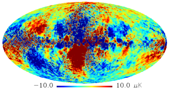
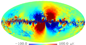
Figure 2: B-modes of the galactic foreground maps (synchrotron + dust) as simulated using v1.6.4 of the PSM. Top: synchrotron-dominated emission at 30 GHz, Bottom: dust-dominated emission at 340 GHz. In spite of the fact that the direction of polarisation of both processes is determined by the same galactic magnetic field, differences in the 3-D distributions and in the depolarisation factors result in quite different B-mode polarisation patterns.

2.2.4 Anomalous dust

If the anomalous dust emission, which may account for a significant part of the intensity emission in the range 10-30 GHz (2004ApJ...614..186F; 2004ApJ...606L..89D; 2008arXiv0802.3345M), can be interpreted as spinning dust grains emission (1998ApJ...508..157D), it should be slightly polarised under 35 GHz (2006ApJ...645L.141B), and only marginally polarised at higher frequencies (2003NewAR..47.1107L). For this reason, it is neglected (and not modelled) here. However, we should keep in mind that there exist other possible emission processes for dust, like the magneto-dipole mechanism, which can produce highly polarised radiation, and could thus contribute significantly to dust polarisation at low frequencies, even if sub-dominant in intensity (2003NewAR..47.1107L).

2.3 Other processes

The left panel in Fig. 1 presents the respective contribution from the various foregrounds as predicted by the PSM at 100 GHz. Synchrotron and dust polarised emission, being by far the strongest contaminants on large scales, are expected to be the main foregrounds for the measurement of primordial B-modes. In this work, we thus mainly focus on the separation from these two diffuse contaminants. However, other processes yielding polarised signals at levels comparable with either the signal of interest, or with the sensitivity of the instrument used for B-mode observation, have to be taken into account.

2.3.1 Free-free

Free-free emission is assumed unpolarised to first order (the emission process is not intrinsically linearly polarised), even if, in principle, low level polarisation by Compton scattering could exist at the edge of dense ionised regions. In WMAP data analysis, Macellari08 find an upper limit of 1% for free–free polarisation. At this level, free-free would have to be taken into account for measuring CMB B-modes for low values of $r$. As this is just an upper limit however, no polarised free-free is considered for the present work.

2.3.2 Extra-galactic sources

Polarised emission from extra-galactic sources is expected to be faint below the degree scale. 2005MNRAS.360..935T, however, estimate that radio sources become the major contaminant after subtraction of the galactic foregrounds. It is, hence, an important foreground at high galactic latitudes. In addition, the point source contribution involves a wide range of emission processes and superposition of emissions from several sources, which makes this foreground poorly coherent across frequencies, and hence difficult to subtract using methods relying on the extrapolation of template emission maps.

The Planck Sky Model provides estimates of the point source polarised emission. Source counts are in agreement with the prediction of 2005A&A...431..893D, and with WMAP data. For radio-sources, the degree of polarisation for each source is randomly drawn from the observed distribution at 20 GHz (2004A&A...415..549R). For infrared sources, a distribution with mean polarisation degree of 0.01 is assumed. For both populations, polarisation angles are uniformly drawn in $[0-2\pi[$. The emission of a number of known galactic point sources is also included in PSM simulations.

2.3.3 Lensing

The last main contaminant to the primordial B-mode signal is lensing-induced B-type polarisation, the level of which should be of the same order as that of point sources (left panel of Fig. 1). For the present work, no sophisticated lensing cleaning method is used. Lensing effects are modelled and taken into account only at the power spectrum level and computed using the CAMB software package, based itself on the CMBFAST software (1998ApJ...494..491Z; 2000ApJS..129..431Z).

2.3.4 Polarised Sunyaev-Zel’dovich effect

The polarised Sunyaev Zel’dovich effect (1999MNRAS.310..765S; 1999MNRAS.305L..27A; Seto05), is expected to be very sub-dominant and is neglected here.

2.4 Uncertainties on the foreground model

Due to the relative lack of experimental constraints from observation at millimetre wavelengths, uncertainties on the foreground model are large. The situation will not drastically improve before the Planck mission provides new observations of polarised foregrounds. It is thus very important to evaluate, at least qualitatively, the impact of such uncertainties on component separation errors for B-mode measurements.

We may distinguish two types of uncertainties, which impact differently the separation of CMB from foregrounds. One concerns the level of foreground emission, the other its complexity.

Quite reliable constraints on the emission level of polarised synchrotron at 23 GHz are available with the WMAP measurement, up to the few degrees scale. Extrapolation to other frequencies and smaller angular scales may be somewhat insecure, but uncertainties take place where this emission becomes weak and sub-dominant. The situation is worse for the polarised dust emission, which is only weakly constrained from WMAP and Archeops at 94 and 353 GHz. The overall level of polarisation is constrained only in the galactic plane, and its angular spectrum is only roughly estimated. In addition, variations of the polarisation fraction (2008arXiv0809.2094D) may introduce significant deviations to the frequency scaling of dust B-modes.

Several processes make the spectral indexes of dust and synchrotron vary both in space and frequency. Some of this complexity is included in our baseline model, but some aspects, like the dependence of the dust polarisation fraction with frequency and the steepening of the synchrotron spectral index, remain poorly known and are not modelled in our main set of simulations. In addition, uncharacterised emission processes have been neglected. This is the case for anomalous dust, or polarisation of the free-free emission through Compton scattering. If such additional processes for polarised emission exist, even at a low level, they would decrease the coherence of galactic foreground emission between frequency channels, and hence our ability to predict the emission in one channel knowing it in the others – a point of much importance for any component separation method based on the combination of multi-frequency observations.

The component separation as performed in this paper, hence, is obviously sensitive to these hypotheses. We will dedicate a part of the discussion to assess the impact of such modelling errors on our conclusions.

3 Estimating $r$ with contaminants

Let us now turn to a presentation of the component separation (and parameter estimation) method used to derive forecasts on the tensor to scalar ratio measurements.

Note that in principle, the best analysis of CMB observations should simultaneously exploit measurements of all fields ($T$, $E$, and $B$), as investigated already by 2007MNRAS.376..739A. Their work, however, addresses an idealised problem. For component separation of temperature and polarisation together, the best approach is likely to depend on the detailed properties of the foregrounds (in particular on any differences, even small, between foreground emissions laws in temperature and in polarisation) and of the instrument (in particular noise correlations, and instrumental systematics). None of this is available for the present study. For this reason, we perform component separation in B-mode maps only. Additional issues such as disentangling $E$ from $B$ in cases of partial sky coverage for instance, or in presence of instrumental systematic effects, are not investigated here either. Relevant work can be found in 2002AIPC..609..209K; 2003NewAR..47..995C; 2003PhRvD..67d3004H; 2007A&A...464..405R.

For low values of tensor fluctuations, the constraint on $r$ is expected to come primarily from the B-mode polarisation. B-modes indeed are not affected by the cosmic variance of the scalar perturbations, contrarily to E-modes and temperature anisotropies. In return, B-mode signal would be low and should bring little constraint on cosmological parameters other than $r$ (and, possibly, the tensor spectral index $n_{t}$, although this additional parameter is not considered here). Decoupling the estimation of $r$ (from B-modes only) from the estimation of other cosmological parameters (from temperature anisotropies, from E-modes, and from additional cosmological probes) thus becomes a reasonable hypothesis for small values of $r$. As we are primarily interested in accurate handling of the foreground emission, we will make the assumption that all cosmological parameters but $r$ are perfectly known. Further investigation of the coupling between cosmological parameters can be found in colombo2008; 2006JCAP...01..019V, and this question is discussed a bit further in Sect. LABEL:sec:tau.

3.1 Simplified approaches

3.1.1 Single noisy map

The first obstacle driving the performance of an experiment being the instrumental noise, it is interesting to recall the limit on $r$ achievable in absence of foreground contamination in the observations.

We thus consider first a single frequency observation of the CMB, contaminated by a noise term $n$:

$$x(\xi)=x^{\text{cmb}}(\xi)+n(\xi)$$ (6)

where $\xi$ denotes the direction in the sky. Assuming that $n$ is uncorrelated with the CMB, the power spectra of the map reads:

$$C_{\ell}=r\mathcal{S}_{\ell}+\mathcal{N}_{\ell}$$

where $\mathcal{S}_{\ell}$ is the shape of the CMB power-spectrum (as set by other cosmological parameters), and $\mathcal{N}_{\ell}$ the power of the noise contamination. Neglecting mode to mode mixing effects from a mask (if any), or in general from incomplete sky coverage, and assuming that $n$ can be modelled as a Gaussian process, the log-likelihood function for the measured angular power spectrum reads:

$$-2\ln\mathcal{L}=\sum_{\ell}(2\ell+1)f_{\text{sky}}\left[\ln\left(\frac{C_{\ell}}{\hat{C}_{\ell}}\right)+\frac{\hat{C}_{\ell}}{C_{\ell}}\right]+\mathrm{const.}$$ (7)

The smallest achievable variance $\sigma_{r}^{2}$ in estimating $r$ is the inverse of the Fisher information $\mathcal{I}=-\operatorname{\mathbf{E}}\left(\frac{\partial^{2}\ln\mathcal{L}}{\partial r^{2}}\right)$ which takes the form:

$$\sigma_{r}^{-2}=\sum_{\ell=\ell_{\min}}^{\ell_{\max}}\frac{2\ell+1}{2}f_{\text{sky}}\left(\frac{\mathcal{S}_{\ell}}{r\mathcal{S}_{\ell}+\mathcal{N}_{\ell}}\right)^{2}$$ (8)

For a detector (or a set of detectors at the same frequency) of noise equivalent temperature $s$ (in $\mu K\sqrt{s}$), and a mission duration of $t_{s}$ seconds, the detector noise power spectrum is $\mathcal{N}_{\ell}=\frac{4\pi s^{2}}{B_{\ell}^{2}t_{s}}\,\mathrm{\mu K}^{2}$, with $B_{\ell}$ denoting the beam transfer function of the detector.

A similar approach to estimating $\sigma_{r}$ is used in 2006JCAP...01..019V where a single ‘cleaned’ map is considered. This map is obtained by optimal combination of the detectors with respect to the noise and cleaned from foregrounds up to a certain level of residuals, which are accounted for as an extra Gaussian noise.

3.1.2 Multi-map estimation

Alternatively, we may consider observations in $F$ frequency bands, and form the $F\times 1$ vector of data $\@vec{x}(\xi)$, assuming that each frequency is contaminated by $\@vec{x}^{\mathrm{cont}}$. This term includes all contaminations (foregrounds, noise, etc…). In the harmonic domain, denoting $\@vec{A}_{\text{cmb}}$ the emission law of the CMB (the unit vector when working in thermodynamic units):

$$\@vec{a}_{\ell m}=\@vec{A}_{\text{cmb}}a_{\ell m}^{\mathrm{cmb}}+\@vec{a}_{\ell m}^{\mathrm{cont}}$$ (9)

We then consider the $F\times F$ spectral covariance matrix $\@tens{R}^{\text{}}_{\ell}$ containing auto and cross-spectra. The CMB signal being uncorrelated with the contaminants, one has:

$$\@tens{R}^{\text{}}_{\ell}=\@tens{R}^{\text{cmb}}_{\ell}+\@tens{N}_{\ell}$$ (10)

with the CMB contribution modelled as

$$\@tens{R}^{\text{cmb}}_{\ell}(r)=r\mathcal{S}_{\ell}\@vec{A}_{\text{cmb}}\@vec{A}_{\text{cmb}}^{\dagger}$$ (11)

and all contaminations contributing a term $\@tens{N}_{\ell}$ to be discussed later. The dagger (${\dagger}$) denotes the conjugate transpose for complex vectors and matrices, and the transpose for real matrices (as $\@vec{A}_{\text{cmb}}$).

In the approximation that contaminants are Gaussian (and, here, stationary) but correlated, all the relevant information about the CMB is preserved by combining all the channels into a single filtered map. In the harmonic domain, the filtering operation reads:

$$\tilde{a}_{\ell m}=\@vec{W_{\ell}}\@vec{a}_{\ell m}=a_{\ell m}^{\mathrm{cmb}}+\@vec{W_{\ell}}\@vec{a}_{\ell m}^{\mathrm{cont}}$$

with

$$\@vec{W}_{\ell}=\frac{\@vec{A}_{\text{cmb}}^{\dagger}{\@tens{N}_{\ell}}^{-1}}{\@vec{A}_{\text{cmb}}^{\dagger}{\@tens{N}_{\ell}}^{-1}\@vec{A}_{\text{cmb}}}$$ (12)

We are back to the case of a single map contaminated by a characterised noise of spectrum:

$$\mathcal{N}_{\ell}=E{|\@vec{W_{\ell}}\@vec{a}_{\ell m}^{\mathrm{cont}}|^{2}}=\left(\@vec{A}_{\text{cmb}}^{\dagger}{\@tens{N}_{\ell}}^{-1}\@vec{A}_{\text{cmb}}\right)^{-1}$$ (13)

If the residual $\@vec{W_{\ell}}\@vec{a}_{\ell m}^{\mathrm{cont}}$ is modelled as Gaussian, the single-map likelihood (7) can be used.

The same filter is used by 2007PhRvD..75h3508A. Assuming that the foreground contribution is perfectly known, the contaminant terms $\@tens{N}_{\ell}$ can be modelled as $\@tens{N}_{\ell}=\@tens{R}^{\text{noise}}_{\ell}+\@tens{R}^{\text{fg}}_{\ell}$. This approach thus permits to derive the actual level of contamination of the map in presence of known foregrounds, i.e. assuming that the covariance matrix of the foregrounds is known.

3.2 Estimating $r$ in presence of unknown foregrounds with SMICA

The two simplified approaches of sections 3.1.1 and 3.1.2 offer a way to estimate the impact of foregrounds in a given mission, by comparing the sensitivity on $r$ obtained in absence of foregrounds (from Eq. 8 when $\mathcal{N}_{\ell}$ contains instrumental noise only), and the sensitivity achievable with known foregrounds (when $\mathcal{N}_{\ell}$ contains the contribution of residual contaminants as well, as obtained from Eq. 13 assuming that the foreground correlation matrix is known).

A key issue, however, is that the solution and the error bar require the covariance matrix of foregrounds and noise to be known. Whereas the instrumental noise can be estimated accurately, assuming prior knowledge of the covariance of the foregrounds to the required precision is optimistic.

To deal with unknown foregrounds, we thus follow a different route which considers a multi-map likelihood (2003MNRAS.346.1089D). If all processes are modelled as Gaussian isotropic, then standard computations yield:

$$-2\ln\mathcal{L}=\sum_{\ell}(2\ell+1)f_{\text{sky}}K\left(\widehat{\@tens{R}}^{\text{}}_{\ell},\@tens{R}^{\text{}}_{\ell}\right)+\text{cst}$$ (14)

where $\widehat{\@tens{R}}^{\text{}}_{\ell}$ is the sample estimate of $\@tens{R}^{\text{}}_{\ell}$:

$$\widehat{\@tens{R}}^{\text{}}_{\ell}=\frac{1}{2\ell+1}\frac{1}{f_{\text{sky}}}\sum_{m=-\ell}^{\ell}\@vec{a}_{l,m}\@vec{a}_{l,m}^{\dagger}$$ (15)

and where $K\left(\cdot,\cdot\right)$ is a measure of mismatch between two positive matrices given by:

$$K\left(\widehat{\@tens{R}}^{\text{}},\@tens{R}^{\text{}}\right)=\frac{1}{2}\left[\operatorname{trace}({\@tens{R}^{\text{}}}^{-1}\widehat{\@tens{R}}^{\text{}})-\operatorname{\log\,\det}({\@tens{R}^{\text{}}}^{-1}\widehat{\@tens{R}}^{\text{}})-F\right]$$ (16)

Expression (14) is nothing but the multi-map extension of (7).

If $\@tens{N}_{\ell}$ is known and fixed, then the likelihood (Eq. 14) depends only on the CMB angular spectrum and can be shown to be equal (up to a constant) to expression 7 with $C_{\ell}=rS_{\ell}$ and $\mathcal{N}_{\ell}$ given by Eq. 13. Thus this approach encompasses both the single map and filtered map approaches.

Unknown foreground contribution can be modelled as the mixed contribution of $D$ correlated sources:

$$\@tens{R}^{\text{fg}}_{\ell}=\@tens{A}\@tens{\Sigma}_{\ell}\@tens{A}^{\dagger}$$ (17)

where $\@tens{A}$ is a $F\times D$ mixing matrix and $\@tens{\Sigma_{\ell}}$ is the $D\times D$ spectral covariance matrix of the sources. The model of the spectral covariance matrix of the observations is then:

$$\@tens{R}^{\text{}}_{\ell}=r\mathcal{S}_{\ell}\@vec{A}_{\text{cmb}}\@vec{A}_{\text{cmb}}^{\dagger}+\@tens{A}\@tens{\Sigma}_{\ell}\@tens{A}^{\dagger}+\@tens{R}^{\text{noise}}_{\ell}$$

We then maximise the likelihood (14) of the model with respect to $r$, $\@tens{A}$ and $\@tens{\Sigma}_{\ell}$.

We note that the foreground parameterisation in Eq.17 is redundant, as an invertible matrix can be exchanged between $\@tens{A}$ and $\@tens{\Sigma}$, without modifying the actual value of $\@tens{R}^{\text{fg}}$. The physical meaning of this is that the various foregrounds are not identified and extracted individually, only their mixed contribution is characterised.

If we are interested in disentangling the foregrounds as well, e.g. to separate synchrotron emission from dust emission, this degeneracy can be lifted by making use of prior information to constrain, for example, the mixing matrix. Our multi-dimensional model offers, however, greater flexibility. Its main advantage is that no assumption is made about the foreground physics. It is not specifically tailored to perfectly match the model used in the simulation. Because of this, it is generic enough to absorb variations in the properties of the foregrounds, as will be seen later-on, but specific enough to preserve identifiability in the separation of CMB from foreground emission. A more complete discussion of the Smica method with flexible components can be found in 2008arXiv0803.1814C.

A couple last details on Smica and its practical implementation are of interest here. For numerical purposes, we actually divide the whole $\ell$ range into $Q$ frequency bins $\mathcal{D}_{q}=\{\ell^{\text{min}}_{q},\cdots,\ell^{\text{max}}_{q}\}$, and form the binned versions of the empirical and true cross power-spectra:

$$\begin{split}\widehat{\@tens{R}}^{\text{}}_{q}&=\frac{1}{w_{q}}\sum_{\ell\in\mathcal{D}_{q}}\sum_{m=-\ell}^{\ell}\@vec{a}_{l,m}\@vec{a}_{l,m}^{\dagger}\\ \@tens{R}^{\text{}}_{q}&=\frac{1}{w_{q}}\sum_{\ell\in\mathcal{D}_{q}}(2\ell+1)\@tens{R}^{\text{}}_{\ell}\end{split}$$ (18)

where $w_{q}$ is the number of modes in $\mathcal{D}_{q}$. It is appropriate to select the domains so that we can reasonably assume for each $\ell\in\mathcal{D}_{q},\@tens{R}^{\text{}}_{\ell}\approx\@tens{R}^{\text{}}_{q}$. This means that spectral bins should be small enough to capture the variations of the power spectra. In practice results are not too sensitive to the choice of the spectral bin widths. Widths between 5 and 10 multipoles constitute a good tradeoff.

Finally, we compute the Fisher information matrix $\@tens{I}_{i,j}(\@vec{\theta})$ deriving from the maximised likelihood (14) for the parameter set $\@vec{\theta}=\left(r,\@tens{A},\@tens{\Sigma_{1}},\cdots,\@tens{\Sigma_{Q}}\right)$:

$$\@tens{I}_{i,j}(\@vec{\theta})=\frac{1}{2}\sum_{q}w_{q}\operatorname{trace}\left(\frac{\partial\@tens{R}^{\text{}}_{q}(\@vec{\theta})}{\partial\theta_{i}}{\@tens{R}^{\text{}}}_{q}^{-1}\frac{\partial\@tens{R}^{\text{}}_{q}(\@vec{\theta})}{\partial\theta_{j}}{\@tens{R}^{\text{}}}_{q}^{-1}\right)$$ (19)

The lowest achievable variance of the $r$ estimate is obtained as the entry of the inverse of the FIM corresponding to the parameter $r$:

$$\sigma_{r}^{2}=\@tens{I}^{-1}_{r,r}$$ (20)

4 Predicted results for various experimental designs

We now turn to the numerical investigation of the impact of galactic foregrounds on the measurements of $r$ with the following experimental designs:

• The Planck space mission, due for launch early 2009, which, although not originally planned for B-mode physics, could provide a first detection if the tensor to scalar ratio $r$ is around $0.1$.

• Various versions of the EPIC space mission, either low cost and low resolution (EPIC-LC), or more ambitious versions (EPIC-CS and EPIC-2m).

• An ambitious (fictitious) ground-based experiment, based on the extrapolation of an existing design (the C$\ell$over experiment).

• An alternative space mission, with sensitivity performances similar to the EPIC-CS space mission, but mapping only a small (and clean) patch of the sky, and referred as the ‘deep field mission’.

The characteristics of these instruments are summed-up in table 1, and Fig. 3 illustrates their noise angular power spectra in polarisation.

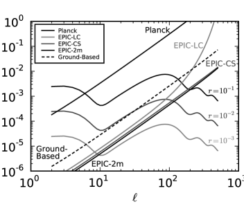
Figure 3: Noise spectra of various experimental designs compared to B-modes levels for $r=0.1$, 0.01 and 0.001. When computing the equivalent multipole noise level for an experiment, we assume that only the central frequency channels contribute to the CMB measurement and that external channels are dedicated to foreground characterisation.

4.1 Pipeline

For each of these experiments, we set up one or more simulation and analysis pipelines, which include, for each of them, the following main steps:

• Simulation of the sky emission for a given value of $r$ and a given foreground model, at the central frequencies and the resolution of the experiment.

• Simulation of the experimental noise, assumed to be white, Gaussian and stationary.

• Computation, for each of the resulting maps, of the coefficients of the spherical harmonic expansion of the B-modes $a^{B}_{\ell m}$

• Synthesis from those coefficients of maps of B-type signal only.

• For each experiment, a mask based on the B-modes level of the foregrounds is built to blank out the brightest features of the galactic emission (see Fig. 4). This mask is built with smooth edges to reduce mode-mixing in the pseudo-spectrum.

• Statistics described in Equation 18 are built from the masked B maps.

• The free parameters of the model described in Sect. 3.2 are adjusted to fit these statistics. The shape of the CMB pseudo-spectrum that enters in the model, is computed using the mode-mixing matrix of the mask (2002ApJ...567....2H).

• Error bars are derived from the Fisher information matrix of the model.

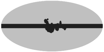
Figure 4: Analysis mask for EPIC B maps, smoothed with a $1^{\circ}$ apodisation window.

Some tuning of the pipeline is necessary for satisfactory foreground separation. The three main free parameters are the multipole range $[\ell_{\text{min}},\ell_{\text{max}}]$, the dimension $D$ of the foreground component, and (for all-sky experiments) the size of the mask.

In practice we choose $\ell_{\text{min}}$ according to the sky coverage and $\ell_{\text{max}}$ according to the beam and the sensitivity. The value of $D$ is selected by iterative increments until the goodness of fit (as measured from the Smica criterion on the data themselves, without knowledge of the input CMB and foregrounds) reaches its expectation. The mask is chosen in accordance to maximise the sky coverage for the picked value of $D$ (see appendix LABEL:sec:d for further discussion of the procedure).

For each experimental design and fiducial value of $r$ we compute three kinds of error estimates which are recalled in Table 4.1.

Knowing the noise level and resolution of the instrument, we first derive from Eq. 8 the error $\sigma_{r}^{\text{noise-only}}$ set by the instrument sensitivity assuming no foreground contamination in the covered part of the sky. The global noise level of the instrument is given by $\mathcal{N}_{\ell}=\left(\@vec{A}_{\text{cmb}}^{\dagger}\@tens{N}_{\ell}^{-1}\@vec{A}_{\text{cmb}}\right)^{-1}$, where the only contribution to $\@tens{N}_{\ell}$ comes from the instrumental noise: $\@tens{N}_{\ell}=\@tens{R}^{\text{noise}}_{\ell}=\operatorname{diag}\left(\frac{4\pi s_{f}^{2}}{B_{\ell},f^{2}t_{s}}\right)$.

In the same way, we also compute the error $\sigma_{r}^{\text{known-foreground}}$ that would be obtained if foreground contribution $\@tens{R}^{\text{fg}}$ to the covariance of the observations was perfectly known, using $\@tens{N}_{\ell}=\@tens{R}^{\text{noise}}_{\ell}+\@tens{R}^{\text{fg}}_{\ell}$. Here we assume that $\@tens{R}^{\text{fg}}=\widehat{\@tens{R}}^{\text{fg}}$ where $\widehat{\@tens{R}}^{\text{fg}}$ is the sample estimate of $\@tens{R}^{\text{fg}}$ computed from the simulated foreground maps.

Finally, we compute the error $\sigma_{r}^{\text{SMICA}}$ given by the Fisher information matrix of the model (Eq. 20).

In each case, we also decompose the FIM in the contribution from large scale modes ($\ell\leq 20$) and the contribution from small scales ($\ell>20$) to give indications of the relative importance of the bump (due to reionisation) and the peak (at higher $\ell$) in the constraint of $r$.

We may notice that in some favourable cases (at low $\ell$, where the foregrounds dominate), the error estimate given by Smica can be slightly more optimistic than the estimate obtained using the actual empirical value of the correlation matrix $\widehat{\@tens{R}}^{\text{fg}}$. This reflects the fact that our modelling hypothesis, which imposes to $\@tens{R}^{\text{fg}}$ to be of rank smaller than $D$, is not perfectly verified in practice (see Appendix LABEL:sec:d for further discussion of this hypothesis). The (small) difference (an error on the estimation of $\sigma_{r}$ when foregrounds are approximated by our model) has negligible impact on the conclusions of this work.

Table 1: Summary of experimental designs.

Experiment	frequency	beam FWHM	NET	$T_{obs}$	sky coverage
	(GHz)	(’)	($\mu K\sqrt{s}$)	(yr)	($f_{sky}$)
PLANCK	30, 44, 70	33, 24, 14	96, 97, 97	1.2	1
	100, 143, 217, 353	10, 7.1, 5, 5	41, 31, 51, 154
EPIC-LC	30, 40, 60	155, 116, 77	28, 9.6, 5.3	2	1
	90, 135, 200, 300	52, 34, 23, 16	2.3, 2.2, 2.3, 3.8
EPIC-CS	30, 45, 70, 100	15.5, 10.3, 6.6, 4.6	19, 8, 4.2, 3.2	4	1
	150, 220, 340, 500	3.1, 2.1, 1.4, 0.9	3.1, 5.2, 25, 210
EPIC-2m	30, 45, 70, 100	26, 17, 11, 8	18, 7.6, 3.9, 3.0	4	1
	150, 220, 340, 500(,800)	5, 3.5, 2.3, 1.5(, 0.9)	2.8, 4.4, 20, 180(, 28k)
Ground-Based	97, 150, 225	7.5, 5.5, 5.5	12, 18, 48	0.8	0.01
Deep field	30, 45, 70, 100	15.5, 10.3, 6.6, 4.6	19, 8, 4.2, 3.2	4	0.01
	150, 220, 340, 500	3.1, 2.1, 1.4, 0.9	3.1, 5.2, 25, 210

Table 2: Error prediction for various experimental designs and fiducial $r$ values. Error bars from the columns noise-only and known foregrounds are derived from Eq.(8) assuming $\@tens{N}_{\ell}=\@tens{R}^{\text{noise}}$ and $\@tens{N}_{\ell}=\@tens{R}^{\text{noise}}+\@tens{R}^{\text{fg}}$ respectively. Error bars from the Smica column are obtained by the inversion of the FIM computed from the Smica model at the point of convergence of the algorithm as in Eq.(20). In all cases, large scale ($\ell\leq 20$) and small scale ($\ell>20$) error bars are computed by decomposing the Fisher information between contribution from low and high multipoles. This allows for an estimation of respective contribution from the bump and the peak to the measurement. The $r^{\text{est}}$ column gives the estimated value at the convergence point in Smica. Detections at more than $4\sigma$ are bold-faced.