Abstract

We show that in supersymmetric models with gauged $B-L$ symmetry, there is a new source for cosmological lepton asymmetry. The Higgs bosons responsible for $B-L$ gauge symmetry breaking decay dominantly into right–handed sneutrinos $\tilde{N}$ and $\tilde{N}^{*}$ producing an asymmetry in $\tilde{N}$ over $\tilde{N}^{*}$. This can be fully converted into ordinary lepton asymmetry in the decays of $\tilde{N}$. In simple models with gauged $B-L$ symmetry we show that resonant/soft leptogenesis is naturally realized. Supersymmetry guarantees quasi–degenerate scalar states, while soft breaking of SUSY provides the needed CP violation. Acceptable values of baryon asymmetry are obtained without causing serious problems with gravitino abundance.

1 Introduction

Baryon number minus lepton number ($B-L$) is a non–anomalous symmetry in the standard model. There is a perception that all non–anomalous symmetries may have a gauge origin. $B-L$ may then be a true gauge symmetry broken spontaneously at a high energy scale. Such a scenario fits well with the small neutrino masses observed in experiments. This is because gauging of $B-L$ requires the introduction of right–handed neutrinos $N_{i}$, one per family, for canceling the triangle anomaly associated with $[U(1)_{B-L}]^{3}$. These $N_{i}$ fields facilitate the seesaw mechanism [1] to generate small neutrino masses. In this context one is able to relate the mass of the heavy right–handed neutrino to the scale of $B-L$ symmetry breaking. With just the standard model gauge symmetry the right–handed neutrinos are not compelling, and even if they are introduced, their bare Majorana masses are not protected and can take values as large as the Planck mass.

In the supersymmetric context there is yet another motivation for gauging $B-L$. It would lead to a natural understanding of $R$–parity [2, 3]. This can be seen by writing the $R$–parity transformation as $R=(-1)^{3(B-L)+2S}$, which clearly shows the close relation between $R$ parity and $B-L$. If the $B-L$ gauge symmetry is broken by Higgs fields carrying even number of $B-L$ charge, then a discrete $Z_{2}$ symmetry will remain unbroken, which would serve as $R$–parity. Such Higgs fields are just the ones needed for generating large Majorana neutrino masses for the right–handed neutrinos, which requires $B-L$ breaking by two units. $R$–parity is usually assumed in MSSM as an ad hoc symmetry, in order to avoid rapid proton decay and to identify the lightest SUSY particle as the cosmological dark matter. These are natural consequences of gauged $B-L$ symmetry. This symmetry also fits inside of $SO(10)$ grand unification, which is very well motivated because of the unification of quarks and leptons of a family into a single multiplet. It is well known that with or without supersymmetry, existence of right–handed neutrinos can explain the observed excess of baryons over antibaryons in the universe via leptogenesis [4]. The $N$ field decays into leptons, generating an asymmetry in lepton number, which is converted to baryon asymmetry by electroweak sphalerons [5]. (For reviews on leptogenesis see [6, 7].)

In this paper we investigate baryogenesis via leptogenesis in supersymmetric models with gauged $B-L$ symmetry. We have identified a new source for leptogenesis in this context. The Higgs fields that spontaneously break $B-L$ symmetry produce an excess of $\tilde{N}$ over $\tilde{N}^{*}$ in their decays, where $\tilde{N}$ stands for the scalar partner of the right-handed neutrino $N$. This asymmetry in $\tilde{N}$ is converted into ordinary lepton asymmetry when the $\tilde{N}$ decays into leptons and Higgs bosons. The electroweak sphalerons convert this lepton asymmetry into baryon asymmetry.

In this scenario, one realizes resonant [8, 9, 10] and soft leptogenesis [11, 12]. Resonant leptogenesis assumes nearly degenerate states (fermions or scalars) that decay into leptons producing an asymmetry which is resonantly enhanced. Usually the needed degeneracy is achieved by postulating additional symmetries. In our context, supersymmetry guarantees near degeneracy of the Higgs states. This comes about since in the SUSY limit, the Higgs scalars responsible for $B-L$ symmetry breaking form partners of a Dirac fermion, leading to two complex (or four real) degenerate scalar states. Once SUSY breaking is turned on, this degeneracy is lifted, but by terms that are suppressed by a factor $M_{\rm susy}/M_{\Delta}$, where $M_{\Delta}$ denotes the mass of the decaying heavy Higgs particle. In the simplest model with gauged $B-L$ symmetry, CP violation needed for leptogenesis is provided by soft SUSY breaking effects. Thus the model realizes soft leptogenesis. We compute the baryon asymmetry generated through this $\tilde{N}$ asymmetry in a simple model with gauged $B-L$ symmetry. As in soft leptogeneis, we find that for a range of soft SUSY breaking parameters, reasonable values of baryon asymmetry can be generated. This mechanism works well when the mass of the decaying Higgs filed is less than about $10^{8}$ GeV. The Davidson–Ibarra bound [13], which requires the decaying right–handed neutrino to be heavier than $10^{9}$ GeV in conventional leptogeneis, is evaded in our framework because the source of CP violation resides in SUSY breaking couplings. Such a bound causes a problem with gravitino abundance [14, 15], which requires the reheat temperature after inflation to be $T_{R}<10^{7}$ GeV. Our scenario does not have the gravitino problem, since the mass of the heavy Higgs particle is $<10^{8}$ GeV. Some of the soft SUSY parameters have to take unusually small values, a situation common with soft leptogenesis, although the parameters that are small in our models are different ones, associated with $B-L$ symmetry breaking.

We present the minimal gauged SUSY model in Sec. 2, work out the spectrum of the model after SUSY breaking in Sec. 3, and compute the cosmological lepton asymmetry in Sec. 4.

2 Minimal Supersymmetric Gauged $B-L$ Model

The minimal supersymmetric model with gauged $B-L$ symmetry extends the gauge group of MSSM to $SU(3)_{C}\times SU(2)_{L}\times U(1)_{Y}\times U(1)_{B-L}$. The triangle anomaly associated with $[U(1)_{B-L}]^{3}$ is canceled by contributions from right–handed neutrinos $N_{i}$, which must exist, one per family. Since the $N_{i}$ fields should be much heavier than the weak scale in order for the seesaw mechanism for small neutrino masses to be effective, we assume that $B-L$ symmetry is broken in the SUSY limit. The simplest set of scalar superfields that would achieve this – if one insists, as we do, on renormalizable coulings – is $\{\overline{\Delta},~{}\Delta,~{}S\}$, where the first two fields carry $B-L$ charges of $\pm 2$, while $S$ is neutral. All three fields are neutral under $SU(3)_{C}\times SU(2)_{L}\times U(1)_{Y}$. The $B-L$ charge of the $\Delta$ field is chosen so that it has direct Yukawa couplings with the $N$ fields, which would provide large Majorana masses for them upon spontaneous symmetry breaking. This choice also guarantees that $R$–parity of MSSM will remain unbroken even after spontaneous symmetry breaking, since $\left\langle\Delta\right\rangle\neq 0$ leaves an unbroken $Z_{2}$ symmetry, which functions as $R$–parity. Our normalization of $B-L$ charge is as follows. $(N,~{}e^{c})$ have charge $+1$, $L$ has charge $-1$, $Q$ has charge $1/3$ while $(u^{c},~{}d^{c})$ fields carry charge $-1/3$. No other fields beyond MSSM fields are introduced.

The superpotential of the model consistent with the extended gauge symmetry is given by

$$W = W_{\rm MSSM}+W^{(B-L)}~{},$$

$$W^{(B-L)} = \lambda S(\Delta\bar{\Delta}-M^{2})+\frac{1}{2}f_{ij}N_{i}N_{j}\Delta+Y_{\nu}^{\alpha i}L_{\alpha}N_{i}H_{u}~{}.$$ (1)

Here $W_{\rm MSSM}$ is the MSSM superpotential. $L_{\alpha}$ denotes the left–handed lepton doublets, $H_{u}$ is the up–type Higgs doublet, and $i,\alpha$ are family indices. Note that all $R$–parity violating couplings are forbidden in the superpotential by the $B-L$ symmetry. The Majorana masses for the right–handed neutrinos arise only after spontaneous breaking of $B-L$ symmetry after $\left\langle\Delta\right\rangle\neq 0$ develops, via the couplings $f_{ij}$. The Dirac Yukawa couplings $Y_{\nu}$ will then generate small neutrino masses via the seesaw mechanism. Bare mass terms for $S$ as well as for $\Delta\overline{\Delta}$ and an $S^{3}$ term have not been written in Eq. (1). This is for simplicity and their omission can be justified by invoking an $R$ symmetry.

We minimize the potential, which contains $F$–terms resulting from Eq. (1) and a $D$–term corresponding to the $B-L$ symmetry, in the SUSY limit. Demanding the vanishing of $F$–terms, $F_{S}=F_{\Delta}=F_{\bar{\Delta}}=0$, yields $\langle S\rangle=0$ and $\langle\Delta\bar{\Delta}\rangle=M^{2}$. The vanishing of the $D$–term implies $|\Delta|=|\bar{\Delta}|$. Without loss of generality we choose $\langle\Delta\rangle=|M|$. Consequently we have $\langle\bar{\Delta}\rangle=|M|e^{i\phi_{M^{2}}}$, with the definition $\phi_{M^{2}}\equiv{\rm arg}(M^{2})$. The spectrum of the model in the SUSY limit consists of a massive vector multiplet ${\cal V}_{B}$ and a pair of degenerate chiral multiplets $(\Delta_{0},~{}S)$ with masses given by

$$M_{\cal V_{B}}=2g_{B}|M|,~{}~{}~{}~{}~{}~{}~{}~{}M_{\Delta}=\sqrt{2}|\lambda||M|~{}.$$ (2)

Here $g_{B}$ denotes the $B-L$ gauge coupling. In this limit, the $B-L$ gaugino pairs up with a Higgsino (denoted $\Delta^{\prime}$) which is a linear combination of $\Delta$ and $\overline{\Delta}$ fields. The orthogonal combination $\Delta_{0}$ pairs up with the $S$–Higgsino to forma a Dirac fermion. Small SUSY breaking effects, to be discussed shortly, will split the masses of the two Weyl components in each of these Dirac fermions. The ($\Delta_{0},~{}S)$ system consists of two complex scalars as well – corresponding to four real nearly degenerate scalar states once small SUSY breaking effects are included, which are physical. It is these nearly degenerate scalar states that will be relevant for leptogenesis.

We will be interested in the limit where the physical Higgs multiplet $(\Delta_{0},~{}S)$ is somewhat lighter than the gauge supermultiplet, that is, in the limit $\sqrt{2}\lambda\ll 2g_{B}$. Precisely how much lighter will be quantified later, but we will not need a larger hierarchy in masses, $M_{\Delta}<0.1~{}M_{\cal V_{B}}$ or so will suffice. With such a mild hierarchy in masses, the dominant decay of the $(\Delta,~{}S)$ Higgs fields will be into right-handed neutrino fields. This will enable a new way of generating lepton asymmetry stored in $\tilde{N}$ fields. With $M_{\Delta}\ll M_{\cal V_{B}}$, we can integrate out the vector supermultiplet to obtain an effective superpotential $W_{\rm eff}$ and an effective Kähler potential $K_{\rm eff}$ involving only the $(\Delta_{0},~{}S)$ fields and the MSSM superfields.

To obtain the effective Lagrangian of the theory after integrating out the vector superfield, we work in the unitary gauge and make supersymmetric transformations on the ($\Delta,~{}\overline{\Delta})$ fields, the gauge vector multiplet ${\cal V}_{B}$, and all fields $\Phi_{i}$ carrying $B-L$ charge $q_{i}$ to go to a new basis with $(\Delta^{\prime},~{}\Delta_{0})$ fields and a shifted ${\cal V}_{B}$ gauge superfield:

$$\Delta = (|M|+\frac{1}{\sqrt{2}}\Delta_{0})e^{q_{\Delta}g_{B}\Delta^{\prime}}~{},~{}~{}~{}~{}~{}~{}~{}\bar{\Delta}=(|M|+\frac{1}{\sqrt{2}}\Delta_{0})e^{-q_{\Delta}g_{B}\Delta^{\prime}+i\phi_{M^{2}}}~{},~{}~{}~{}$$

$${\cal V}_{B} = {\cal V}_{B}^{0}-\Delta^{\prime}-{\Delta^{\prime}}^{{\dagger}}~{},~{}~{}~{}~{}~{}~{}~{}~{}~{}~{}~{}~{}~{}~{}~{}~{}~{}\Phi_{i}\to e^{q_{i}g_{B}\Delta^{\prime}}\Phi_{i}~{}.$$ (3)

We have kept the $B-L$ charge of $\Delta,~{}\overline{\Delta}$ fields as $(q_{\Delta},~{}-q_{\Delta})$ to be more general.

With these redefinitions, the original Kähler Lagrangian, given by

$${\cal L}_{D}^{(B-L)}=\int d^{4}\theta\left(\Delta^{{\dagger}}e^{q_{\Delta}g_{B}{\cal V}_{B}}\Delta+\bar{\Delta}^{{\dagger}}e^{-q_{\Delta}g_{B}{\cal V}_{B}}\bar{\Delta}+\sum_{i}\Phi_{i}^{{\dagger}}e^{q_{i}g_{B}{\cal V}_{B}}\Phi_{i}\right)~{}$$ (4)

transforms into

$${\cal L}_{D}^{(B-L)}=\int d^{4}\theta\left(\left\{2|M|^{2}+\sqrt{2}|M|(\Delta_{0}+\Delta_{0}^{{\dagger}})+\Delta_{0}^{{\dagger}}\Delta_{0}\right\}{\rm Cosh}(q_{\Delta}g_{B}{\cal V}_{B}^{0})+\sum_{i}\Phi_{i}^{{\dagger}}e^{q_{i}g_{B}{\cal V}_{B}^{0}}\Phi_{i}\right)~{}.$$ (5)

Observe that the $\Delta^{\prime}$ field has disappeared in Eq. (5), it has been eaten up by the gauge superfield ${\cal V}_{B}^{0}$. In the process the gauge field ${\cal V}_{B}^{0}$ becomes massive, all its components acquiring a mass $M_{\cal V_{B}}^{2}=q_{\Delta}^{2}g^{2}|M|^{2}$, as can be readily seen by expanding the Cosh function in Eq. (5).

Now we can integrate out the massive gauge superfiled ${\cal V}_{B}^{0}$. We obtain the following effective Kähler Lagrangian:

$${\cal L}_{\rm D,eff}^{(B-L)} = \int d^{4}\theta\left[\Delta_{0}^{{\dagger}}\Delta_{0}+\sum_{i}\Phi_{i}^{{\dagger}}\Phi_{i}-\frac{1}{4q_{\Delta}^{2}|M|^{2}}\left(\sum_{i}q_{i}\Phi_{i}^{{\dagger}}\Phi_{i}\right)^{2}\right.$$ (6)

$$\left.+\frac{\Delta_{0}\!+\!\Delta_{0}^{{\dagger}}}{4\sqrt{2}q_{\Delta}^{2}|M|^{3}}\left(\!\sum_{i}q_{i}\Phi_{i}^{{\dagger}}\Phi_{i}\!\right)^{2}\!\!\!+\frac{1}{8q_{\Delta}^{2}|M|^{4}}(\Delta_{0}^{{\dagger}}\Delta_{0}\!-\Delta_{0}^{2}\!-\Delta_{0}^{{\dagger}2})\left(\!\sum_{i}q_{i}\Phi_{i}^{{\dagger}}\Phi_{i}\!\right)^{2}+\cdots\right],$$

where the $\cdots$ indicate terms with higher powers of $1/|M|$. Eq. (6) describes the interactions of the light $\Delta_{0}$ field with other light MSSM fields through the exchange of the gauge supermultiplet. Notice that these interactions are suppressed by $1/|M|^{3}$.

With the redefinition of fields given in Eq. (3), the superpotential of Eq. (1) becomes $W_{\rm eff}=W_{\rm MSSM}+W(\Delta_{0},N)$ with

$$W(\Delta_{0},N)=\lambda Se^{i\phi_{M^{2}}}\left(|M|\sqrt{2}\Delta_{0}+\frac{1}{2}\Delta_{0}^{2}\right)+\frac{1}{2}f_{ij}(|M|+\frac{1}{\sqrt{2}}\Delta_{0})N_{i}N_{j}+Y_{\nu}^{\alpha i}L_{\alpha}N_{i}H_{u}~{}.$$ (7)

Note that the $\Delta^{\prime}$ field has disappeared in Eq. (7). Majorana masses for $N$ have been generated with $M_{N_{i}}=|f_{i}||M|$, where $|f_{i}|$ are the real and diagonal eigenvalues of the matrix $f_{ij}$. It is also clear from Eq. (7) that $(\tilde{\Delta}_{0},~{}\tilde{S})$ fields pair up to form a Dirac fermion with a mass given by $M_{\Delta}=\sqrt{2}|\lambda||M|$. Their scalar partners $(\Delta_{0},~{}S)$ are of course degenerate with these fermions, since SUSY breaking has not yet been turned on.

We assume that at least one of the $N_{i}$ fields is lighter than $\Delta_{0}$. Such situation is quite natural, especially when the $N_{i}$ fields have hierarchical masses. We denote this light $N_{i}$ field simply as $N$ (assuming for simplicity that only one such field is lighter than $\Delta_{0}$) with its mass given by $M_{N}=|fM|$. The dominant decays of $\Delta_{0}$ scalar will then be $\Delta_{0}\rightarrow\tilde{N}+\tilde{N}$, $\Delta_{0}\rightarrow\tilde{N}^{*}\tilde{N}^{*}$, and $\Delta_{0}\rightarrow NN$. There is also a subdominant decay of $\Delta_{0}$ into $\tilde{N}\tilde{N}^{*}$. Here $N$ denotes the right–handed neutrino, while $\tilde{N}$ stands for its scalar partner. Supersymmetry will dictate that the decays of the fermionic partner of $\Delta_{0}$, denoted as $\tilde{\Delta}_{0}$ will be to $\tilde{N}N$ and $\tilde{N}^{*}N$ final states with an identical width. The total width for the decays of the scalar $\Delta_{0}$ is given by

$$\Gamma(\Delta_{0}\rightarrow\tilde{N}\tilde{N}+\tilde{N}^{*}\tilde{N}^{*}+\tilde{N}\tilde{N}^{*}+NN)={|f|^{2}\over 64\pi}M_{\Delta}\sqrt{1-{4M_{N}^{2}\over M_{\Delta}^{2}}}~{}.$$ (8)

Since in our scheme, lepton asymmetry is initially created as an asymmetry in $\tilde{N}$ versus $\tilde{N}^{*}$, we are interested in range of model parameters where these decays are essentially out-of-equilibrium at temperatures around the mass of $\Delta_{0}$. For $M_{\Delta}\sim(10^{6}-10^{8})$ GeV, this requirement implies that $|f|$ in Eq. (8) should obey $|f|\leq 2\cdot(10^{-5}-10^{-4})$. For such small values of $|f|$, it is important to check if the gauge boson mediated decays of $\Delta_{0}$ will have a comparable rate. To check this, we have computed the total decay width of $\Delta_{0}$ scalars into four MSSM fields. These could be four scalars, four fermions, or two scalars plus two fermions, all of the MSSM. The total width is given by

$$\Gamma(\Delta_{0}\rightarrow\Phi_{i}^{*}\Phi_{i}\Phi_{j}^{*}\Phi_{j})={256\times 4(g_{B}/2)^{6}\over 360\times(2\pi)^{5}}\left({M_{\Delta}^{7}\over M_{\cal V_{B}}^{6}}\right)~{}.$$ (9)

In Eq. (9), $\Phi_{i}$ stands for any of the scalar or fermion fields of MSSM. The factor $256$ arises as $[{\rm Tr}(q_{i}^{2})]^{2}$, while the factor 4 is to account for the various types of final states stated above. We see that these decays are suppressed by phase space and inverse power of the ${\cal V_{B}}$ mass. If we demand that the decays of $\Delta_{0}$ given in Eq. (8) dominates over the ones in Eq. (9), we arrive at an inequality $(g_{B}/2)M_{\Delta}/M_{\cal V_{B}}<1.6|f|^{1/3}$, or using Eq. (2), $|\lambda|\leq 4.5|f|^{1/3}$. If $|f|=10^{-5}$, this translates into a limit $|\lambda|\leq 0.1$. This a rather mild hierarchy, which is quite natural. We will henceforth assume that the two body decay of $\Delta_{0}$ into $\tilde{N}\tilde{N}$ dominates over the four body decay, which would enable us to create lepton asymmetry in $\tilde{N}$.

3 Spectrum including SUSY breaking

In the supersymmetric limit we have seen that four real scalar fields belonging to the $(\Delta_{0},~{}S)$ superfileds are degenerate in mass. The corresponding fermions are also degenerate in mass. This degeneracy will be lifted once SUSY breaking interactions are taken into account. One would arrive at two quasi–degenerate Majorana fermions and four quasi–degenerate real scalar fields. Their mass splittings and coupling to the $(N,~{}\tilde{N}$) fields are crucial for the estimation of the induced lepton asymmetry in $\tilde{N}$. Here and in the next section we compute these splittings and couplings.

Soft supersymmetry breaking interactions are introduced in the usual way as in supergravity. For the $(\Delta,~{}\overline{\Delta},~{}S,~{}N)$ sector the relevant soft breaking terms are given by

$$V_{\rm soft}=\{A_{\lambda}\lambda S\Delta\overline{\Delta}-C_{\lambda}\lambda M^{2}S+{A_{f}f_{ij}\over 2}\Delta\tilde{N}_{i}\tilde{N}_{j}+h.c.\}+m_{i}^{2}\Phi_{i}^{*}\Phi_{i}~{}.$$ (10)

The dimensional parameters $\{A_{\lambda},~{}A_{f},~{}C_{\lambda}\}$ will be taken to have values near the TeV scale. Mass–splittings within degenerate multiplets will be induced at order $M_{\rm susy}\sim$ TeV, so we will ignore terms of order $M_{\rm susy}^{2}$ and higher. The soft squared mass parameters $m_{i}^{2}$ in Eq. (10) can then be neglected.

We now minimize the potential including soft SUSY breaking, keeping linear terms in $M_{\rm susy}$. First we obtain the redefined soft breaking terms after the transformation of Eq. (3) is applied to Eq. (10). This yields

$$V_{\rm soft}=\lambda M^{2}(A_{\lambda}-C_{\lambda})S+A_{\lambda}\lambda e^{i\phi_{M^{2}}}S(\sqrt{2}|M|\Delta_{0}+\frac{1}{2}\Delta_{0}^{2})+\frac{1}{2}A_{f}f_{ij}(|M|+\frac{1}{\sqrt{2}}\Delta_{0})\tilde{N}_{i}\tilde{N}_{j}+{\rm h.c.}+m_{i}^{2}|\Phi_{i}|^{2}~{}.$$ (11)

The full potential is given by $V=V_{F}+V_{\rm Soft}$, with $V_{F}$ obtained from Eq. (7) as

$$V_{F}=|\lambda\Delta_{0}|^{2}|\sqrt{2}|M|+\frac{1}{2}\Delta_{0}|^{2}+|\lambda\sqrt{2}|M|S+\lambda S\Delta_{0}+\frac{e^{-i\phi_{M^{2}}}}{2\sqrt{2}}f_{ij}\tilde{N}_{i}\tilde{N}_{j}|^{2}+|f_{ij}(|M|+\frac{1}{\sqrt{2}}\Delta_{0})\tilde{N}_{j}|^{2}~{},$$ (12)

where we have neglected terms arising from $Y_{\nu}$ coupling.

Minimization of $V$ shows that the field $S$ develops a vacuum expectation value (VEV) of order $M_{\rm susy}$ given by

$$\langle S^{*}\rangle=\frac{C_{\lambda}-A_{\lambda}}{2\lambda^{*}}e^{i\phi_{M^{2}}}~{}.$$ (13)

The shift in the VEV of the $\Delta_{0}$ field is of order $M_{\rm susy}^{2}$ and thus negligible. As a consequence of $\left\langle S\right\rangle\neq 0$, the mass matrix in the fermion sector spanning $(\tilde{\Delta}_{0},~{}\tilde{S})$ gets modified. We now have this matrix given by

$$\begin{array}[]{cc}&{\begin{array}[]{cc}&\end{array}}\\ \vspace{1mm}\hskip 2.84544pt{\cal M}_{fermi}=e^{i(\phi_{M^{2}}+\phi_{\lambda})}\begin{array}[]{c}\\ {}{}{}\hfil\end{array}\!\!\!\!\!&{\left(\begin{array}[]{cc}|\lambda|\left\langle S\right\rangle&M_{\Delta}\\ M_{\Delta}&0\end{array}\right)}~{}.\end{array}\!\!~{}~{}~{}~{}~{}$$ (14)

Here we have denoted the phase of $\lambda$ as $\phi_{\lambda}$. Eq. (14) leads to two quasi–degenerate Majorana fermions with masses given by $M_{\psi_{1,2}}=M_{\Delta}\pm|\lambda\left\langle S\right\rangle|/2$.

In the bosonic sector, the squared mass matrix spanning $\left({\rm Re}(\Delta_{0}),{\rm Re}(S),{\rm Im}(\Delta_{0}),{\rm Im}(S)\right)$, is found to be (to order $M_{\rm susy}$)

$$\begin{array}[]{cccc}&{\begin{array}[]{cccc}&&&\end{array}}\\ \vspace{1mm}\hskip 2.84544pt{\cal M}^{2}_{boson}=M_{\Delta}^{2}\begin{array}[]{c}\\ {}{}\hfil\\ {}{}\hfil\\ {}\hfil\end{array}\!\!\!\!\!&{\left(\begin{array}[]{cccc}1&\kappa_{R}+\kappa^{\prime}_{R}&0&\kappa_{I}-\kappa^{\prime}_{I}\\ \kappa_{R}+\kappa^{\prime}_{R}&1&-\kappa^{\prime}_{I}&0\\ 0&-\kappa^{\prime}_{I}&1&-\kappa^{\prime}_{R}\\ \kappa_{I}-\kappa^{\prime}_{I}&0&-\kappa^{\prime}_{R}&1\end{array}\right)}~{},\end{array}\!\!~{}~{}~{}~{}~{}$$ (15)

$${\rm with}~{}~{}~{}(\kappa_{R},\kappa_{I},\kappa^{\prime}_{R},\kappa^{\prime}_{I})=\frac{\sqrt{2}}{|M|}\left({\rm Re}(\left\langle S\right\rangle),~{}{\rm Im}(\left\langle S\right\rangle),~{}{\rm Re}(\frac{A_{\lambda}e^{i\phi_{M^{2}}}}{2\lambda^{*}}),~{}{\rm Im}(\frac{A_{\lambda}e^{i\phi_{M^{2}}}}{2\lambda^{*}})\right)~{}.$$ (16)

The eigenvalues of the matrix in Eq. (15) are found to be:

$$M_{X_{1,2}}^{2}=M_{\Delta}^{2}\left(1\pm\Delta_{12}+\Delta_{14}\right)~{},~{}~{}~{}~{}M_{X_{3,4}}^{2}=M_{\Delta}^{2}\left(1\mp\Delta_{12}-\Delta_{14}\right)$$ (17)

with the definitions

$$\Delta_{12}=-\frac{|C_{\lambda}+A_{\lambda}|}{2M_{\Delta}}~{},~{}~{}~{}~{}~{}\Delta_{14}=\frac{|C_{\lambda}-A_{\lambda}|}{2M_{\Delta}}~{}.$$ (18)

Thus $\Delta_{12}=(M_{X_{1}}^{2}-M_{X_{2}}^{2})/(2M_{\Delta}^{2})$ parametrizes the fractional mass splitting in $X_{1}$ and $X_{2}$, and similarly $\Delta_{14}$ in $X_{1}$ and $X_{4}$. These two mass splittings will be relevant for leptogenesis calculation. We also note the identities $\Delta_{12}=\Delta_{43}$ and $\Delta_{14}=\Delta_{23}$. There are two other mass splittings which can be obtained in terms of $\Delta_{12}$ and $\Delta_{14}$, but those two turn out to be not relevant for leptogenesis.

The mass eigenstates $X_{i}$ are related to the original states as

$${\rm Re}(\Delta_{0}) = \frac{c_{\alpha}}{\sqrt{2}}(X_{1}+X_{3})+\frac{s_{\alpha}}{\sqrt{2}}(X_{2}+X_{4})~{},~{}~{}~{}{\rm Re}(S)=\frac{c_{\beta}}{\sqrt{2}}(X_{1}-X_{3})+\frac{s_{\beta}}{\sqrt{2}}(X_{2}-X_{4})~{},$$

$${\rm Im}(\Delta_{0}) = -\frac{s_{\alpha}}{\sqrt{2}}(X_{1}+X_{3})+\frac{c_{\alpha}}{\sqrt{2}}(X_{2}+X_{4})~{},~{}~{}~{}{\rm Im}(S)=-\frac{s_{\beta}}{\sqrt{2}}(X_{1}-X_{3})+\frac{c_{\beta}}{\sqrt{2}}(X_{2}-X_{4}).$$ (19)

Here two mixing angles appear which we denote as ($\alpha,\beta$). We use the notation $c_{\alpha}=\cos\alpha,~{}s_{\alpha}=\sin\alpha$, etc. These two angles are given by

$$\alpha=\frac{1}{2}\left(\pi+{\rm arg}(C_{\lambda}+A_{\lambda})-{\rm arg}(C_{\lambda}-A_{\lambda})\right)~{},~{}~{}~{}\beta=\frac{\pi}{2}+\phi_{M^{2}}+\phi_{\lambda}+\frac{1}{2}\left({\rm arg}(C_{\lambda}+A_{\lambda})+{\rm arg}(C_{\lambda}-A_{\lambda})\right)~{}.$$ (20)

We shall use these results in the next section where we compute the lepton asymmetry stored in $\tilde{N}$ arising from the decays of these scalar states.

4 Cosmological lepton asymmetry

In our scenario, cosmological lepton asymmetry is generated in the out of equilibrium decays of the $X_{i}$ scalars into $\tilde{N}$ and $\tilde{N}^{*}$, the scalar partners of the right–handed neutrino. One loop corrections to the decay induces CP asymmetry, leading to an asymmetry in $\tilde{N}$ versus $\tilde{N}^{*}$. This induced asymmetry is converted to usual lepton asymmetry when $\tilde{N}$ and $\tilde{N}^{*}$ decay into leptons and a Higgs boson, which subsequently is converted to baryon asymmetry via electroweak sphaleron processes.

As shown in Sec. 2, the dominant decay of the $X_{i}$ scalars will be into final states with $\tilde{N}$ scalars and $N$ fermions, with a smallish coupling $\lambda\leq 0.1$ and $|f|\sim 10^{-5}$. The tree level decay diagrams are shown in Fig. 1. The total decay rate for these decays is given in Eq. (8). The decay of $X_{i}$, which are real scalars, into final states with opposite lepton number ($-2$ and $+2$) (see Fig. 1 (a) and (b)) raises the possibility that an asymmetry can be produced in $\tilde{N}$ number. For $M_{\Delta}=10^{6}-10^{8}$ GeV and $|f|=10^{-5}-10^{-4}$, the lepton number violating decays of the $X_{i}$ fields will be out of equilibrium. The efficiency factor in the production of $\tilde{N}$ asymmetry will then be nearly one.

Figure 1: Tree level decays of $X_{i}$ scalars into $\tilde{N},\tilde{N}^{*}$ and $N$.

We now proceed to calculate the induced $\tilde{N}$ asymmetry. For this purpose we need to identify the interaction of the $X_{i}$ fields with $\tilde{N}$. Since the $X_{i}$ fields are quasi–degenerate, the dominant contribution to lepton asymmetry will arise from wave function corrections shown in Fig. 2. These corrections have a resonance enhancement, which is lacking in the vertex correction diagrams. SUSY provides the quasi–degeneracy of $X_{i}$ fields, which enables us to realize resonant leptogenesis in $\tilde{N}$. The required CP violation arises in the model from soft SUSY breaking couplings. Thus this scenario is also soft leptogenesis, but with four $X_{i}$ fields involved in the decay.

From the Lagrangian given in Eqs. (11) and (12), one can read off the cubic scalar interactions relevant for the wave function corrections of Fig. 2. The couplings of $X_{i}$ to $\tilde{N}$ is found to be

$$V^{(3)}=\left(\tilde{N}\tilde{N}F_{\tilde{N}\tilde{N}i}X_{i}+{\rm h.c.}\right)+|\tilde{N}|^{2}F_{|\tilde{N}|i}X_{i}~{},$$ (21)

where we have defined

$$F_{\tilde{N}\tilde{N}i} = \frac{f}{4\sqrt{2}}\left(a_{1}\!+\!a_{2}\!+\!M_{\Delta}e^{i\omega},~{}-i(a_{1}\!-\!a_{2}\!+\!M_{\Delta}e^{i\omega}),~{}a_{1}\!+\!a_{2}\!-\!M_{\Delta}e^{i\omega},~{}-i(a_{1}\!-\!a_{2}\!-\!M_{\Delta}e^{i\omega})\right)_{i}$$

$$F_{|\tilde{N}|i} = \frac{|f||M_{N}|}{\sqrt{2}}\left(c_{\alpha},~{}s_{\alpha},~{}c_{\alpha},~{}s_{\alpha}\right)_{i}$$

$${\rm with}~{} ~{}a_{1}=\frac{C_{\lambda}-A_{\lambda}}{2}e^{i\alpha}~{},~{}~{}~{}~{}a_{2}=A_{f}e^{-i\alpha}~{},~{}~{}~{}~{}\omega=\beta-\phi_{\lambda}-\phi_{M^{2}}~{}.$$ (22)

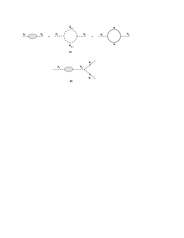
Figure 2: Loop diagrams generating CP asymmetry in the decay $X_{i}\rightarrow\tilde{N}^{*}\tilde{N}^{*}$. The blob in (b) corresponds to the resummed two point functions shown in (a).

The $\tilde{N}$ and $\tilde{N}^{*}$ states mix after SUSY breaking. This splitting effect will show up in the loops of Fig. 2. To take these effects into account, we go to the mass eigenbasis of these states $\tilde{N}_{+}$ and $\tilde{N}_{-}$ which are given by

$$\tilde{N}_{+}=\frac{1}{\sqrt{2}}(e^{ix}\tilde{N}+e^{-ix}\tilde{N}^{*})~{},~{}~{}~{}~{}\tilde{N}_{-}=\frac{1}{\sqrt{2}i}(e^{ix}\tilde{N}-e^{-ix}\tilde{N}^{*})~{}.$$ (23)

The phase parameter $x$ in Eq. (23) is defined as $x=\frac{1}{2}\left(\phi_{f}+{\rm arg}(A_{f}+\frac{C_{\lambda}-A_{\lambda}}{2})\right).$ Note that $\tilde{N}_{\pm}$ are real fields with masses given by

$$M_{\tilde{N}_{+}}^{2}=|M_{N}|^{2}+|M_{N}|\left|A_{f}+\frac{C_{\lambda}-A_{\lambda}}{2}\right|~{},~{}~{}~{}~{}M_{\tilde{N}_{-}}^{2}=|M_{N}|^{2}-|M_{N}|\left|A_{f}+\frac{C_{\lambda}-A_{\lambda}}{2}\right|~{}.$$ (24)

In the $\tilde{N}_{a}=(\tilde{N}_{+},\tilde{N}_{-})$ ($a=\pm$) basis, the cubic scalar interactions can be written as

$$V^{(3)}=(\tilde{N}_{+}^{2}F_{++\hskip 1.42262pti}+\tilde{N}_{-}^{2}F_{--\hskip 1.42262pti}+\tilde{N}_{+}\tilde{N}_{-}F_{+-\hskip 1.42262pti})X_{i}~{},$$ (25)

where

$$F_{++i} = \frac{1}{2}\left(e^{-2ix}F_{\tilde{N}\tilde{N}i}+e^{2ix}F_{\tilde{N}\tilde{N}i}^{*}+F_{|\tilde{N}|i}\right)~{},~{}~{}~{}F_{--i}=-\frac{1}{2}\left(e^{-2ix}F_{\tilde{N}\tilde{N}i}+e^{2ix}F_{\tilde{N}\tilde{N}i}^{*}-F_{|\tilde{N}|i}\right)~{},$$

$$F_{+-i} = i\left(e^{-2ix}F_{\tilde{N}\tilde{N}i}-e^{2ix}F_{\tilde{N}\tilde{N}i}^{*}\right)~{}.$$ (26)

It is now straightforward to work out the absorptive part of the two point function arising from diagrams with $\tilde{N}$’s in the loops. We find it to be

$$\Pi_{ij}^{B}(p^{2}) = \frac{1}{32\pi}\left(2K_{++}F_{++\hskip 1.42262pti}F_{++\hskip 1.42262ptj}+2K_{--}F_{--\hskip 1.42262pti}F_{--\hskip 1.42262ptj}+K_{+-}F_{+-\hskip 1.42262pti}F_{+-\hskip 1.42262ptj}\right)~{},$$

$${\rm where}~{}~{}~{}~{} K_{ab}=\left(1-2\frac{M_{\tilde{N}_{a}}^{2}\!+\!M_{\tilde{N}_{b}}^{2}}{p^{2}}+\frac{(M_{\tilde{N}_{a}}^{2}\!-\!M_{\tilde{N}_{b}}^{2})^{2}}{p^{4}}\right)^{1/2}$$ (27)

When considering $X_{i}$-decay, one should set $p^{2}=M_{X_{i}}^{2}$.

We will also need the Yukawa couplings of the $X_{i}$ fields with the $N$ fermions. It is given by

$${\cal L}_{NNY} = NNY_{F}X+{\rm h.c.}$$

$${\rm with}~{}~{} ~{}Y_{F}=\frac{fe^{-i\alpha}}{4\sqrt{2}}\left(1,~{}i,~{}1,~{}i\right)~{}.$$ (28)

The absorptive part arising through the fermionic loop in Fig. 2 is found to be

$$\Pi_{ij}^{F}(p^{2})=\frac{1}{16\pi}\sqrt{1-4\frac{M_{N}^{2}}{p^{2}}}\left[p^{2}(Y_{F}^{{\dagger}}Y_{F}+Y_{F}^{T}Y_{F}^{*})_{ij}-2M_{N}^{2}(Y_{F}^{T}Y_{F}e^{-2i\phi_{f}}+Y_{F}^{\dagger}Y_{F}^{*}e^{2i\phi_{f}})_{ij}\right]~{}.$$ (29)

With these, we have for example, for the absorptive part of $\Pi_{12}$,

$$\Pi_{12}=\Pi_{12}^{B}+\Pi_{12}^{F}\simeq\frac{|f|^{2}}{32\pi}\frac{\hat{A_{1}}}{4M_{\Delta}}\sqrt{1-4\frac{M_{N}^{2}}{M_{\Delta}^{2}}}M_{\Delta}^{2}~{},$$ (30)

where $\hat{A_{1}}$ is defined in Eq. (33).

We now combine these results to compute $\epsilon_{\tilde{N}}$, the $\tilde{N}$ asymmetry parameter defined as

$$\epsilon_{\tilde{N}}=\sum_{i}{\Gamma(X_{i}\rightarrow\tilde{N}\tilde{N})-\Gamma(X_{i}\rightarrow\tilde{N}^{*}\tilde{N}^{*})\over\Gamma(X_{i}\rightarrow\tilde{N}\tilde{N})+\Gamma(X_{i}\rightarrow\tilde{N}^{*}\tilde{N}^{*})}~{}.$$ (31)

We find it to be

$$\epsilon_{\tilde{N}}=4\left[\frac{2\Delta_{12}\Gamma/M_{\Delta}}{4\Delta_{12}^{2}+(\frac{\Gamma}{2M_{\Delta}})^{2}}\cdot\frac{\hat{A}_{1}}{M_{\Delta}}+\frac{2\Delta_{14}\Gamma/M_{\Delta}}{4\Delta_{14}^{2}+(\frac{\Gamma}{2M_{\Delta}})^{2}}\cdot\frac{\hat{A}_{2}}{M_{\Delta}}\right]~{},$$ (32)

where $\Gamma$ is a total decay width [i.e. $\Gamma(X_{i}\to{\rm everything})$]. Here we have defined two effective $A$–parameters as follows:

$$\hat{A}_{1} = |A_{f}|\sin\phi_{1}-2\left|A_{f}+\frac{C_{\lambda}-A_{\lambda}}{2}\right|\frac{(M_{N}/M_{\Delta})^{2}}{1-4(M_{N}/M_{\Delta})^{2}}\sin\phi_{2}$$

$$\hat{A}_{2} = -2\left|A_{f}+\frac{C_{\lambda}-A_{\lambda}}{2}\right|\frac{(M_{N}/M_{\Delta})^{2}}{1-4(M_{N}/M_{\Delta})^{2}}\sin\phi_{3}$$ (33)

The phases appearing in Eq. (32) are related to the original phases in the model through the relations

$$\phi_{1}={\rm arg}(A_{f})-{\rm arg}(C_{\lambda}+A_{\lambda})~{},~{}~{}~{}\phi_{2}={\rm arg}(A_{f}+{C_{\lambda}-A_{\lambda}\over 2})-{\rm arg}(C_{\lambda}+A_{\lambda})~{},$$

$$\phi_{3}={\rm arg}(A_{f}+{C_{\lambda}-A_{\lambda}\over 2})-{\rm arg}(C_{\lambda}-A_{\lambda})~{}.$$ (34)

It should be mentioned that the asymmetry given in Eq. (32) includes fermionic and bosonic loop contributions. It turns out that the fermionic loop is entirely canceled by the bosonic loop, the left-over piece from the bosonic loop is what is given in Eq. (32). This cancelation is not surprising, since the fermion loop corrections do not feel the effects of SUSY breaking. We also note that the off–diagonal $\Pi_{ij}$ have one power of $M_{\rm susy}/M_{X}$ suppression, so the decay vertex has to be supersymmetric. This feature simplifies the calculations somewhat. In Eq. (32) we have added the asymmetry arising from all four of the $X_{i}$ scalar fields.

In principle, the decays of the Higgsinos $(\tilde{\Delta}_{0},\tilde{S})$ into $\tilde{N}$ and $N$ can create an asymmetry in $\tilde{N}$. However, we find that there is not sufficient CP violation in these decays in the minimal model.

Now we are ready to estimate the lepton asymmetry created by $\tilde{N}$-decays at the second stage where $\tilde{N}$ decays into a lepton and a Higgs boson. Note that lepton asymmetry between $\tilde{N}$ and $\tilde{N}^{*}$ will be completely converted into lepton asymmetry in the MSSM sector. There is however one peculiarity related to SUSY. $\tilde{N}$ has two primary decay channels $\tilde{N}\to L\tilde{H}_{u}$ and $\tilde{N}\to\tilde{L}^{*}H_{u}^{*}$. Since the rates of these processes are the same due to SUSY (at zero temperature), the lepton asymmetries created from these decays cancel each other. However, with $T\neq 0$ the cancelation is only partial (due to temperature effects which explicitly break SUSY) and one has

$$\tilde{\epsilon}=\epsilon(\tilde{N}\to L\tilde{H}_{u})\Delta_{BF}~{},$$ (35)

with the temperature dependent factor $\Delta_{BF}$ given in Ref. [6]. Now, the baryon asymmetry created from the lepton asymmetry due to $\tilde{N}$ decays is:

$$\frac{\tilde{n}_{B}}{s}\simeq-8.6\cdot 10^{-4}\frac{\tilde{\epsilon}}{\Delta_{BF}}\eta=-8.6\cdot 10^{-4}\epsilon_{\tilde{N}}\eta~{},$$ (36)

where we have taken into account an effective number of degrees of freedom, including one RHN superfield, to be $g_{*}=225$. In the last stage of Eq. (36) we have substituted $\tilde{\epsilon}$ by $\epsilon_{\tilde{N}}$ - the $\tilde{N}$ asymmetry created at the first stage by $X_{i}$-decays. $\eta$ is an efficiency factor which depends on $\tilde{m}\simeq\frac{v_{u}^{2}}{M}Y_{\nu}^{2}$, and which takes into account temperature effects by integrating the Boltzmann equations [6]. For instance, efficiency $\eta$ reaches its maximal value, $\eta\approx 0.1$ for $\tilde{m}\approx 10^{-3}$ eV. Thus, in order to generate the experimentally observed asymmetry $\left(\frac{n_{B}}{s}\right)_{\rm exp}=(8.75\pm 0.23)\cdot 10^{-11}$, we need to have $\epsilon_{\tilde{N}}\stackrel{{\scriptstyle>}}{{{}_{\sim}}}10^{-6}$. Going back to Eq. (32), we see that an enhancement of $\epsilon_{\tilde{N}}$ will happen for small values of $\Delta_{ij}$. The natural values of these parameters are $\sim M_{susy}/M_{\Delta}$. However, some cancelation can make either of these parameters smaller. Assuming that this happens for $\Delta_{12}$, with the parametrization $\Delta_{12}=\delta_{12}M_{susy}/M_{\Delta}$ and $\hat{A}_{1}=\delta_{1}M_{susy}$ we have $\epsilon_{\tilde{N}}\approx 2\delta_{1}\Gamma/(\delta_{12}M_{\Delta})$. On the other hand, out of equilibrium decay of $X_{i}$ states requires $\Gamma\stackrel{{\scriptstyle<}}{{{}_{\sim}}}H=1.7\sqrt{g_{*}}M_{\Delta}^{2}/M_{\rm Pl}$. Therefore, we have $\epsilon_{\tilde{N}}\stackrel{{\scriptstyle<}}{{{}_{\sim}}}3.4\sqrt{g_{*}}\delta_{1}M_{\Delta}/(\delta_{12}M_{\rm Pl})$. With the choice $\delta_{1}\approx 3$ and $\delta_{12}\approx 1/300$ and $M_{\Delta}\simeq 10^{8}$ GeV, we obtain $\epsilon_{\tilde{N}}\simeq 10^{-6}$. This has been achieved by the suppressed value $\delta_{12}$, which does not seem to be natural. Similar situation occurs in the soft leptogenesis scenario. However, note that within our setup we do not need to constrain the value of the Dirac Yukawa coupling $Y_{\nu}$ very much. The only real constraint is that $\tilde{N}$ decays out of equilibrium, which requires $\Gamma\stackrel{{\scriptstyle<}}{{{}_{\sim}}}H$.

We conclude with a few remarks. We have kept corrections linear in $M_{\rm susy}/M_{\Delta}$ in the computation of CP asymmetry, and not any higher powers. It is known that if the mass of the decaying field is close to the SUSY scale, second order vertex corrections can be important proportional to the mass of the MSSM gaugino [16]. In our scheme, these vertex corrections do not exist, since the $B-L$ gaugino has decoupled and since $\tilde{N}$ does not couple to MSSM gauginos. A natural question to ask is whether the soft SUSY breaking corrections that induce lepton asymmetry can also lead to excessive CP violation in electron and neutron dipole moments. With universal soft breaking mass parameters there is a potential problem. We note that if the theory is embedded in SUSY left–right model, then all the Dirac Yukawa couplings and $A$–terms are hemitian due to parity symmetry. That will make all EDM contributions vanishingly small [17]. On the other hand, parity symmetry implies that the Majorana–type couplings (such as $A_{f}$ and $f$ in our model) are complex symmetric, which can serve to induce the lepton asymmetry.

References

• [1] P. Minkowski, Phys. Lett. B 67 (1977) 421;
M. Gell-Mann, P. Ramond and R. Slansky, in it Supergravity eds. P. van Nieuwenhuizen and D.Z. Freedman (North Holland, Amsterdam, 1979) p. 315;
T. Yanagida, In Proceedings of the Workshop on the Baryon Number of the Universe and Unified Theories, Tsukuba, Japan, 13-14 Feb 1979;
S. L. Glashow, NATO Adv. Study Inst. Ser. B Phys.  59 (1979) 687;
R. N. Mohapatra and G. Senjanovic, Phys. Rev. Lett.  44 (1980) 912;
See also J. Schechter and J. W. F. Valle, Phys. Rev.  D 22 (1980) 2227.
• [2] R. N. Mohapatra, Phys. Rev.  D 34 (1986) 3457;
A. Font, L. E. Ibanez and F. Quevedo, Phys. Lett.  B 228 (1989) 79;
S. P. Martin, Phys. Rev.  D 46 (1992) 2769.
• [3] C. S. Aulakh, A. Melfo and G. Senjanovic, Phys. Rev.  D 57 (1998) 4174.
• [4] M. Fukugita and T. Yanagida, Phys. Lett.  B 174 (1986) 45.
• [5] V. A. Kuzmin, V. A. Rubakov and M. E. Shaposhnikov, Phys. Lett.  B 155 (1985) 36.
• [6] G. F. Giudice, A. Notari, M. Raidal, A. Riotto and A. Strumia, Nucl. Phys.  B 685 (2004) 89.
• [7] W. Buchmuller, P. Di Bari and M. Plumacher, Annals Phys.  315 (2005) 305;
S. Davidson, E. Nardi and Y. Nir, Phys. Rept.  466 (2008) 105.
• [8] M. Flanz, E. A. Paschos, U. Sarkar and J. Weiss, Phys. Lett.  B 389 (1996) 693.
• [9] A. Pilaftsis, Phys. Rev.  D 56 (1997) 5431.
• [10] A. Pilaftsis and T. E. J. Underwood, Nucl. Phys.  B 692 (2004) 303.
• [11] Y. Grossman, T. Kashti, Y. Nir and E. Roulet, Phys. Rev. Lett.  91 (2003) 251801.
• [12] G. D’Ambrosio, G. F. Giudice and M. Raidal, Phys. Lett.  B 575 (2003) 75.
• [13] S. Davidson and A. Ibarra, Phys. Lett.  B 535 (2002) 25.
• [14] M. Y. Khlopov and A. D. Linde, Phys. Lett.  B 138 (1984) 265;
J. R. Ellis, D. V. Nanopoulos and S. Sarkar, Nucl. Phys.  B 259 (1985) 175.
• [15] K. Kohri, T. Moroi and A. Yotsuyanagi, Phys. Rev.  D 73 (2006) 123511.
• [16] Y. Grossman, T. Kashti, Y. Nir and E. Roulet, JHEP 0411 (2004) 080;
C. S. Fong and M. C. Gonzalez-Garcia, arXiv:0901.0008 [hep-ph].
• [17] K. S. Babu, B. Dutta and R. N. Mohapatra, Phys. Rev.  D 61 (2000) 091701 [arXiv:hep-ph/9905464].