Two-dimensional nonlinear vector states in Bose-Einstein condensates

Abstract

Two-dimensional (2D) vector matter waves in the form of soliton-vortex and vortex-vortex pairs are investigated for the case of attractive intracomponent interaction in two-component Bose-Einstein condensates. Both attractive and repulsive intercomponent interactions are considered. By means of a linear stability analysis we show that soliton-vortex pairs can be stable in some regions of parameters while vortex-vortex pairs turn out to be always unstable. The results are confirmed by direct numerical simulations of the 2D coupled Gross-Pitaevskii equations.

I Introduction

Multicomponent Bose-Einstein condensates (BECs) have been subject of growing interest in recent years as they open intriguing possibilities for a number of important physical applications, including coherent storage and processing of optical fields op1 ; op2 , quantum simulation qubit , quantum interferometry etc. Experimentally, multicomponent BECs can be realized by simultaneous trapping of different species of atoms DifAtom1 ; DifAtom2 or atoms of the same isotope in different hyperfine states. Magnetic trapping freezes spin dynamics MagTrap1 ; MagTrap2 , while in optical dipole traps all hyperfine states are liberated (spinor BECs) OpTrap1 . Theoretical models of multicomponent BECs in the mean-field approximation are formulated in the framework of coupled Gross-Pitaevskii (GP) equations Dalfovo and the order parameter of multicomponent BECs is described by a multicomponent vector.

Like in the scalar condensate case, various types of nonlinear matter waves have been predicted in multicomponent BECs. They include, in addition to ground-state solutions ground1 ; ground2 ; ground3 , structures which are peculiar to multicomponent BECs only, such as bound states of dark-bright darkbright and dark-dark darkdark , dark-gray, bright-gray, bright-antidark and dark-antidark darkgrey complexes of solitary waves, domain wall solitons wall1 ; wall2 ; wall3 , soliton molecules Molecul , symbiotic solitons symbiotic . Two-dimensional (2D) and three-dimensional (3D) vector solitons and vortices have been considered in Refs. Skryabin ; Garcia1 ; Garcia2 for the case of repulsive condensates. Attractive intracomponent interaction have, on the other hand, received less attention and only one-dimensional vector structures have been studied so far attract1D ; Dutton . Two-dimensional and 3D cases, however, demands special attention since the phenomenon of collapse is possible in attractive BECs.

Interactions between the atoms in the same and different states can be controlled (including changing the sign of the interactions) via a Feshbach resonance. Theoretical and experimental studies have shown that inter-component interaction plays a crucial role in dynamics of nonlinear structures in multicomponent BECs. Recently, two-component BECs with tunable inter-component interaction were realized experimentally exp1 ; exp2 . Note that in nonlinear optics, where similar model equations (without the trapping potential) are used to describe the soliton-induced waveguides Kivshar , the nonlinear coefficients are always of the same sign.

The aim of this paper is to study 2D nonlinear localized vector structures in the form of soliton-vortex and vortex-vortex pairs in a binary mixture of disc-shaped BECs with attractive intracomponent and attractive or repulsive intercomponent interactions. Then, by means of a linear stability analysis, we investigate the stability of these structures and show that pairs of soliton and single-charged vortex can be stable both for attractive and repulsive interactions between different components. Vortex-vortex pairs turn out to be always unstable. The results are confirmed by direct numerical simulations of the 2D coupled Gross-Pitaevskii equations.

The paper is organized as follows. In Sec.  II we formulate a model and present basic equations. The cases of attractive and repulsive intercomponent interactions are considered in Secs.  III and  IV respectively. The conclusions are made in Sec.  V.

II Basic equations

We consider a binary mixture of BECs, consisting of two different spin states of the same isotope. We assume that the nonlinear interactions are weak relative to the confinement in the longitudinal (along $z$-axis) direction. In this case, the BEC is a ”disk-shaped” one, and the GP equations take an effectively 2D form

$$i\hbar\frac{\partial\Psi_{1}}{\partial t}=\left[-\frac{\hbar^{2}}{2M}\nabla^{2}+V_{\mathrm{ext}}(\mathbf{r})+g_{11}|\Psi_{1}|^{2}+g_{12}|\Psi_{2}|^{2}\right]\Psi_{1},$$ (1)

$$i\hbar\frac{\partial\Psi_{2}}{\partial t}=\left[-\frac{\hbar^{2}}{2M}\nabla^{2}+V_{\mathrm{ext}}(\mathbf{r})+g_{21}|\Psi_{1}|^{2}+g_{22}|\Psi_{2}|^{2}\right]\Psi_{2},$$ (2)

where $M$ is the mass of the atoms, $V_{\mathrm{ext}}(\mathbf{r})=M\omega_{\perp}^{2}(x^{2}+y^{2})/2$ is the harmonic external trapping potential with frequency $\omega_{\perp}$ and $\nabla^{2}=\partial^{2}/\partial x^{2}+\partial^{2}/\partial y^{2}$ is the 2D Laplacian. Atom-atom interactions are characterized by the coupling coefficients $g_{ij}=4\pi\hbar^{2}a_{ij}/M$, where $a_{ij}=a_{ji}$ are the $s$-wave scattering lengths for binary collisions between atoms in internal states $|i\rangle$ and $|j\rangle$. Note that $g_{11}=g_{22}$ and $g_{12}=g_{21}$. Introducing dimensionless variables $(x,y)\to(x/l,y/l)$, $t\to\omega_{\perp}t$, $\Psi_{j}\to\Psi_{j}\sqrt{\hbar\omega_{\perp}/(2|g_{11}|)}$, $B_{12}=-g_{12}/|g_{11}|$, $B_{11}=-g_{11}/|g_{11}|$, where $l=\sqrt{\hbar/(M\omega_{\perp})}$, one can rewrite equations (1) and (2) as

$$i\frac{\partial\Psi_{1}}{\partial t}=\left[-\nabla^{2}+x^{2}+y^{2}-|\Psi_{1}|^{2}-B_{12}|\Psi_{2}|^{2}\right]\Psi_{1},$$ (3)

$$i\frac{\partial\Psi_{2}}{\partial t}=\left[-\nabla^{2}+x^{2}+y^{2}-B_{12}|\Psi_{1}|^{2}-|\Psi_{2}|^{2}\right]\Psi_{2}.$$ (4)

In what follows we consider attractive interaction between atoms of the same species and set $B_{11}=B_{22}=1$. We neglect the spin dynamics (assuming magnetic trapping) so that the interaction conserves the total number $N_{j}$ ($j=1,2$) of particles of each component

$$N_{j}=\int{|\Psi_{j}|^{2}d^{2}\textbf{r}},$$ (5)

and energy

$$E=E_{1}+E_{2}-\frac{1}{2}B_{12}\int{|\Psi_{1}|^{2}|\Psi_{2}|^{2}d^{2}\textbf{r}},$$ (6)

where

$$E_{j}=\int\left\{|\nabla\Psi_{j}|^{2}-\frac{1}{2}|\Psi_{j}|^{4}+(x^{2}+y^{2})|\Psi_{j}|^{2}\right\}d^{2}\textbf{r}.$$ (7)

III Attractive intercomponent interaction

III.1 Stationary soliton-vortex pairs

We look for stationary solutions of Eqs. (3) and (4) in the form

$$\Psi_{j}(\mathbf{r},t)=\psi_{j}(r)e^{-i\mu_{j}t+im_{j}\varphi}$$ (8)

where $m_{j}$ is the topological charge (vorticity) of the $j$-th component, $\mu_{j}$ is the chemical potential, $r=\sqrt{x^{2}+y^{2}}$ and $\varphi$ is the polar angle. Substituting Eq. (8) into Eqs. (3) and (4), we have

$$\mu_{1}\psi_{1}+\Delta_{r}^{(m_{1})}\psi_{1}-r^{2}\psi_{1}+(|\psi_{1}|^{2}+B_{12}|\psi_{2}|^{2})\psi_{1}=0,$$ (9)

$$\mu_{2}\psi_{2}+\Delta_{r}^{(m_{2})}\psi_{2}-r^{2}\psi_{2}+(B_{12}|\psi_{1}|^{2}+|\psi_{2}|^{2})\psi_{2}=0,$$ (10)

where $\Delta_{r}^{(m)}=d^{2}/dr^{2}+(1/r)(d/dr)-m^{2}/r^{2}$. As was pointed out the inter-component interaction may be varied over wide range, however, the strength of the intercomponent interaction is weaker than the intracomponent counterpart in most experiments with two-component BECs. Thus $B_{12}$ can be considered as the free parameter from the range $-1\leq B_{12}\leq 1$. We find that the qualitative behavior of vector state characteristics does not change when varying $B_{12}$. To make it definite we further fixed the strength of intercomponent interaction at $B_{12}=\pm 0.5$ for attractive and repulsive cases respectively. In this section we consider the case of attractive interatomic interaction $B_{12}>0$.

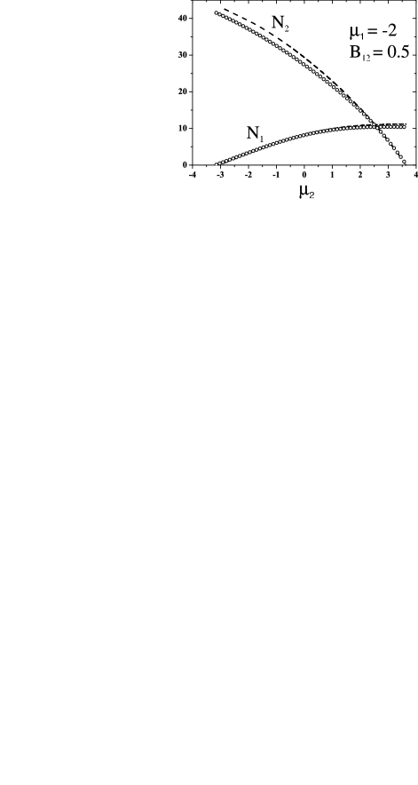
Figure 1: Normalized numbers of atoms $N_{1}$ and $N_{2}$ of each component versus chemical potential $\mu_{2}$ at fixed $\mu_{1}$ for vector soliton-vortex pair ($m_{1}=0$, $m_{2}=1$) (attractive intercomponent interaction).

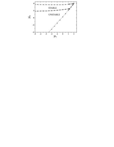
Figure 2: Existence domain for vector state $m_{1}=0$ and $m_{2}=1$ on the $(\mu_{1},\mu_{2})$ plane for attractive intercomponent interaction $B_{12}=0.5$. Open circles correspond to numerically found existence boundaries. Dashed curves outline the variational predictions. At upper and lower boundaries of the existence domain the vector states degenerate into the pure scalar states with $N_{1}=0$ and $N_{2}=0$ respectively. The solid line with triangles indicates the stability boundary.

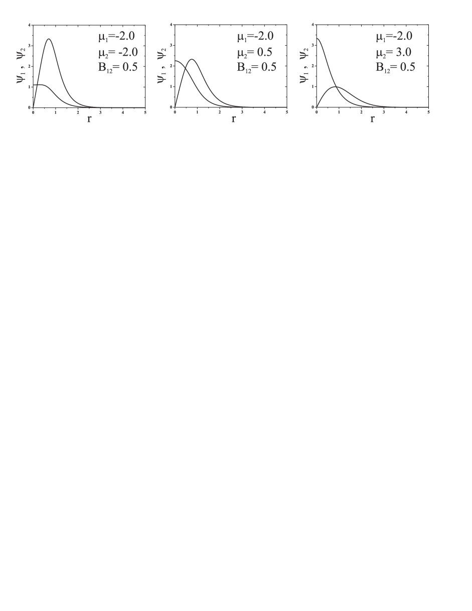
Figure 3: The numerically found solutions of Eqs. (9) and (10) for attractive intercomponent interactions $B_{12}>0$ at fixed $\mu_{1}=-2$ for different values of $\mu_{2}$.

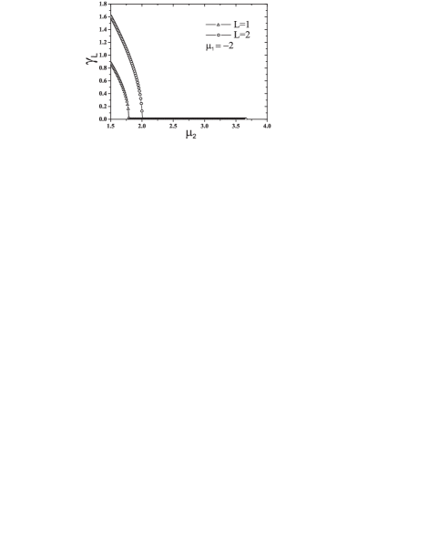
Figure 4: Typical dependence of maximum growth rates for $L=1$ and $L=2$ azimuthal modes as functions of $\mu_{2}$ at fixed $\mu_{1}$, (here $\mu_{1}=-2$), $B_{12}=0.5$. Note that the widest instability domain has $L=2$ mode.

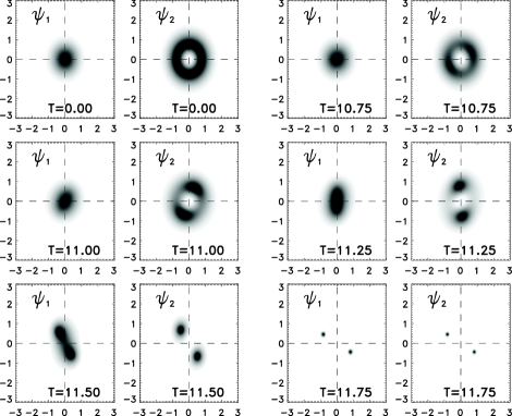
Figure 5: Snapshots of unstable evolution for vector pair $m_{1}=0$, $m_{2}=1$, $\mu_{1}=-2$, $\mu_{2}=0.5$, $B_{12}=0.5$. The absolute values of $|\psi_{1}|$ and $|\psi_{2}|$ are shown in grayscale: the darker regions correspond to higher amplitudes.

First, we present a variational analysis. Stationary solutions of Eqs. (9) and (10) in the form Eq. (8) realize the extremum of the energy functional $E$ under the fixed number of particles $N_{1}$ and $N_{2}$. We take trial functions $\psi_{j}$ in the form

$$\psi_{j}(r)=h_{j}\left(\frac{r}{a_{j}}\right)^{|m_{j}|}\exp{\left(-\frac{r^{2}}{2a_{j}^{2}}+im_{j}\varphi\right)},$$ (11)

which correspond to the localized state $(m_{1},m_{2})$ with vorticities $m_{1}$ and $m_{2}$ for $|1\rangle$ and $|2\rangle$ components respectively, $a_{j}$ and $h_{j}$ are unknown parameters to be determined by the variational procedure. The parameters $h_{1}$ and $h_{2}$ can be excluded using the normalization conditions (5), which yield the relation $N_{j}=m_{j}!\pi h_{j}^{2}a_{j}^{2}$. Thus, the only variational parameters are $a_{1}$ and $a_{2}$. Substituting Eq. (11) into Eq. (III.1), we get for the functional $E$

$$E=E_{1}+E_{2}+E_{12},$$

where

$$E_{j}=\frac{N_{j}}{a_{j}^{2}}\left(m_{j}+1-\frac{N_{j}^{2}(2m_{j})!}{\pi 4^{1+m_{j}}(m_{j}!)^{2}}\right)+N_{j}a_{j}^{2}(m_{j}+1),$$

and

$$E_{12}=-\frac{1}{2}B_{12}N_{1}N_{2}\frac{a_{1}^{2|m_{1}|}a_{2}^{2|m_{2}|}}{(a_{1}^{2}+a_{2}^{2})^{1+|m_{1}|+|m_{2}|}}\frac{(m_{1}+m_{2})!}{\pi m_{1}!m_{2}!}.$$

By solving the variational equations $\partial E/\partial a_{j}=0$ at fixed $N_{j}$ one finds the parameters of approximate solutions with different $m_{1}$ and $m_{2}$. We will focus on one particular configuration with $m_{1}=0$ and $m_{2}=1$ which corresponds to the pair soliton-vortex. The results of the variational analysis for this case and $B_{12}>0$ are given in Fig. 1 and Fig. 2 by dashed lines. These results were the starting point for numerical analysis.

The equations (9) and (10) were discretized on the equidistant radial grid and the resulting system was solved by the stabilized iterative procedure similar to that described in Ref. Petviashvili86 . The appropriate initial guesses were based on the variational approximation. The numerical results are shown in Fig. 1 and Fig. 2 by open circles. It is seen that the variational results exhibit a good agreement with numerical calculations.

The stationary vector states form two-parameter family with parameters $\mu_{1}$ and $\mu_{2}$. In the Fig. 1 the number of atoms for each component of the stationary vector state $(0,1)$ is represented as a function of the chemical potential $\mu_{2}$ at fixed value of $\mu_{1}$. The existence domain is bounded and its boundaries are determined by the condition $\left.\mu_{2}\right|_{N_{1}=0}\leq\mu_{2}\leq\left.\mu_{2}\right|_{N_{2}=0}$. For each value of $\mu_{1}$, where the solution exists, a dependence similar to one presented in Fig. 1 can be found. This allows one to reconstruct an existence domain of the vector pair $(0,1)$ on ($\mu_{1}$, $\mu_{2}$) plane, which is shown in the Fig. 2. As is known, (see e.g. MihalacheMalomedPRA06 ) for the two-dimensional scalar solitary structures in BEC with attraction, the chemical potential is bounded from above $\mu<\mu_{\mathrm{{max}}}=2(m+1)$, where $m$ is the topological charge, and $N\to 0$ when $\mu\to\mu_{\mathrm{{max}}}$. One can see from Fig. 2 that the value of $\mu_{\mathrm{{max}}}$ is reduced in the presence of the second component if the intercomponent interaction is attractive ($B_{12}>0$). Both components vanish at the point $(\mu_{1},\mu_{2})=(2m_{1}+2,2m_{2}+2)$.

Examples of soliton-vortex $(0,1)$ radial profiles are given in Fig. 3. It is interesting to note that when the amplitude of the vortex component is sufficiently high, a soliton profile develops a noticeable plateau. Such a deviation from gaussian-like shape leads to comparable divergence of numerical and variational dependencies in Fig. 1. Other vector states as $(0,2)$, $(-1,1)$, $(-2,2)$ etc. were also found, but they all turn out to be always unstable (see below).

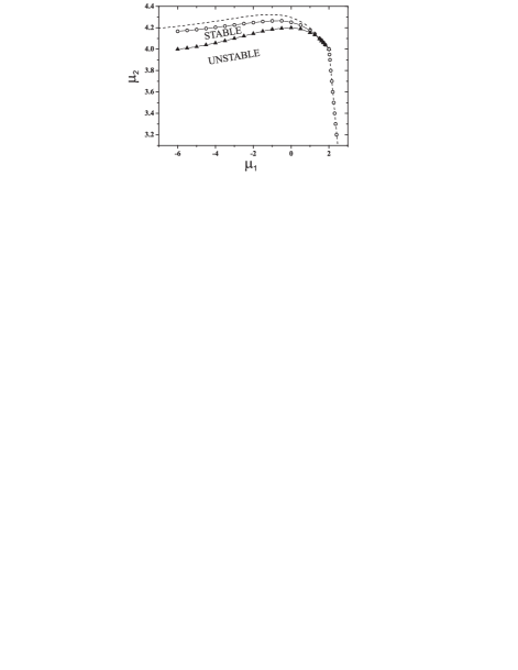
Figure 6: The same as in Fig. 2 for repulsive intercomponent interaction ($B_{12}=-0.5$).

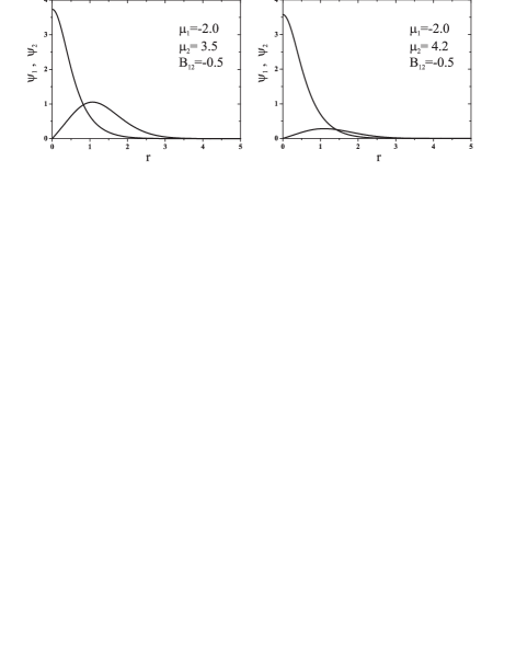
Figure 7: Numerically found solutions of Eqs. (9) and (10) for repulsive intercomponent interactions at fixed $\mu_{1}=-2$ from stable (right panel) and unstable (left panel) regions.

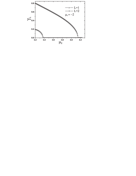
Figure 8: Same as in Fig. 4 for $B_{12}=-0.5$. Note that in contrast to the case of attractive intercomponent interaction the stability threshold is determined by $L=1$ mode.

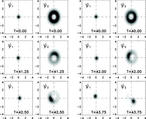
Figure 9: Development of snake-type instability ($L=1$) for vector pair $m_{1}=0$, $m_{2}=1$, $\mu_{1}=-2$, $\mu_{2}=3.5$. Intercomponent interaction is repulsive, $B_{12}=-0.5$. The absolute values of $|\psi_{1}|$ and $|\psi_{2}|$ are shown for different times.

III.2 Stability of stationary solutions

The stability of the vector pairs can be investigated by the analysis of small perturbations of the stationary states. We take the wave functions in the form

$$\Psi_{j}(\textbf{r},t)=\left\{\psi_{j}(r)+\varepsilon_{j}(\textbf{r},t)\right\}e^{-i\mu_{j}t+im_{j}\varphi},$$ (12)

where the stationary solutions $\psi_{j}(r)$ are perturbed by small perturbations $\varepsilon_{j}(\textbf{r},t)$, and linearize Eqs. (3) and (4) with respect to $\varepsilon_{j}$. The basic idea of such a linear stability analysis is to represent a perturbation as the superposition of the modes with different azimuthal symmetry. Since the perturbations are assumed to be small, stability of each linear mode can be studied independently. Presenting the perturbations in the form

$$\varepsilon_{j}(\textbf{r},t)=u_{j}(r)e^{i\omega t+iL\varphi}+v_{j}^{*}(r)e^{-i\omega^{*}t-iL\varphi},$$

we get the following linear eigenvalue problem

$$\left(\begin{array}[]{cccc}\hat{L}_{12}^{(+)}&\alpha_{1}&\beta_{12}&\beta_{12}\\ -\alpha_{1}&-\hat{L}_{12}^{(-)}&-\beta_{12}&-\beta_{12}\\ \beta_{12}&\beta_{12}&\hat{L}_{21}^{(+)}&\alpha_{2}\\ -\beta_{12}&-\beta_{12}&\alpha_{2}&-\hat{L}_{21}^{(-)}\\ \end{array}\right)U=\omega U,$$ (13)

where $U=(u_{1},v_{1},u_{2},v_{2})$ is the vector eigenmode and $\omega$ is an (generally, complex) eigenvalue, $\alpha_{j}=\psi_{j}^{2}$, $\beta_{12}=B_{12}\psi_{1}\psi_{2}$, $\hat{L}_{ij}^{(\pm)}=\mu_{i}+\Delta_{r}^{(m_{i}\pm L)}-r^{2}+2\psi_{i}^{2}+B_{ij}\psi_{j}^{2}$. An integer $L$ determines the number of the azimuthal mode. Nonzero imaginary parts in $\omega$ imply the instability of the state $|\psi_{1},\psi_{2}\rangle$ with $\gamma_{L}=\max|\mathrm{Im}\,\omega|$ being the instability growth rate.

Employing a finite difference approximation, we numerically solved the eigenvalue problem (13). Typical dependencies of the growth rate $\gamma_{L}$ of the azimuthal perturbation modes $L=1$ and $L=2$ on $\mu_{2}$ at fixed $\mu_{1}$ are shown in Fig. 4 for the state $(0,1)$. Note that above some critical value of $\mu_{2}$ all growth rates vanish granting the stability of the vector pair $(0,1)$ against the azimuthal perturbations. For the case of attractive intercomponent interaction $B_{12}>0$ the stability boundary is determined by $L=2$ mode. Similar dependencies of the growth rate $\gamma_{L}$ on $\mu_{2}$ have been obtained for other values of $\mu_{1}$. We have performed the numerical calculation of $\gamma_{L}$ for values of the azimuthal index up to $L=5$. In all studied cases azimuthal stability is always defined by vanishing of the growth rate of $L=2$ mode. The corresponding stability threshold is given in Fig. 2 by filled triangles. Note that in the degenerate scalar case $\psi_{1}=0$ for single-charge vortex $m_{2}=1$ the stability threshold $\mu_{2}=2.552$ coincides with the value obtained in Ref. MihalacheMalomedPRA06 . For the vector states $(0,2)$, $(-1,1)$, $(-2,2)$, the growth rates are found to be nonzero in the entire existence domain and these pairs appear to be always unstable.

To verify the results of the linear analysis, we solved numerically the dynamical equations (3) and (4) initialized with our computed vector solutions. Numerical integration was performed on the rectangular Cartesian grid with a resolution $512^{2}$ by means of standard split-step fourier technique (for details see e.g. KivsharAgrawal ). In full agreement with the linear stability analysis, the states $(0,1)$ perturbed by the azimuthal perturbations with different $L$ survive over huge times provided that the corresponding $\mu_{1}$ and $\mu_{2}$ belong to the stability region. On the other hand, Fig. 5 shows the temporal development of azimuthal $L=2$ instability for the vector state $(0,1)$ with $\mu_{1}=-2$ and $\mu_{2}=0.5$ (i. e. in the instability region). One can see the two humps which appear on the initially smooth ring-like intensity distribution. Further, the vortex profile is deformed, vortex and fundamental soliton both split into two filaments which then collapse. Note that unstable $(0,1)$ pair in BECs with repulsive intracomponent interaction Garcia1 does not collapse and undergo a complex dynamics with trapping one component by another.

IV Repulsive intercomponent interaction

In this section we present results for the case of repulsive interactions $B_{12}<0$ between different components. The existence domain, stable and unstable branches on the $(\mu_{1},\mu_{2})$ plane for the state $(0,1)$ are shown in Fig. 6. It is seen that the repulsive intercomponent interaction leads to an increase of the maximum chemical potential $\mu_{\mathrm{{max}}}$ for each component compared to the case $\mu=4$ of pure scalar solution. The stability properties of the vector states were investigated by the linear stability analysis described in the preceding section. The states $(0,2)$, $(-1,1)$, $(-2,2)$ are always unstable as in the case of $B_{12}>0$.

Figure 7 shows examples of the radial profiles of unstable and stable $(0,1)$ states. In Fig. 8 we plot the growth rates $\gamma_{L}$ as functions of $\mu_{2}$ under fixed $\mu_{1}$ for the azimuthal perturbations with $L=1$ and $L=2$. The growth rates vanish if $\mu_{2}$ exceeds a some critical value. In contrast to the attractive intercomponent interaction case, it is seen that the stability boundary is controlled by the elimination of the snake-type instability (i. e. azimuthal perturbation with $L=1$). Indeed, the repulsion between components naturally leads to spatial separation of condensate species. This relative motion destroys the vector state as seen from Fig. 9.

V Conclusions

In conclusion, we have analyzed the stability of 2D vector matter waves in the form of soliton-vortex and vortex-vortex pairs in two-component Bose-Einstein condensates with attractive interactions between atoms of the same species. Both attractive and repulsive intercomponent interactions are considered. We have performed a linear stability analysis and showed that, in both cases, only soliton-vortex pairs $(0,1)$ can be stable in some regions of parameters. Namely, under the fixed number of atoms in the soliton component, the number of atoms of the vortex component should be less than a some critical value. No stabilization regions have been found for vortex-vortex pairs and they turn out to be always unstable. The results of the linear analysis have been confirmed by direct numerical simulations of the 2D coupled Gross-Pitaevskii equations.

References

- (1) Z. Dutton and L. V. Hau, Phys. Rev. A 70, 053831 (2004).
- (2) C. Liu, Z. Dutton, C. H. Behroozi, and L. V. Hau, Nature (London) 409, 490 (2001); D. F. Phillips, A. Fleischhauer, A. Mair, R. L. Walsworth, and M. D. Lukin, Phys. Rev. Lett. 86, 783 (2001).
- (3) K. T. Kapale and J. P. Dowling, Phys. Rev. Lett. 95, 173601 (2005).
- (4) G. Modugno, G. Ferrari, G. Roati, R.J. Brecha, A. Simoni, and M. Inguscio, Science 294, 1320 (2001); G. Modugno, M. Modugno, F. Riboli, G. Roati, and M. Inguscio, Phys. Rev. Lett. 89, 190404 (2002); G. Modugno, G. Roati, F. Riboli, F. Ferlaino, R.J. Brecha, and M. Inguscio, Science 297, 2240 (2002).
- (5) M. Mudrich, S. Kraft, K. Singer, R. Grimm, A. Mosk, and M. Weidemuller, Phys. Rev. Lett. 88, 253001 (2002).
- (6) D.S. Hall, M.R. Matthews, J.R. Ensher, C.E. Wieman, and E.A. Cornell, Phys. Rev. Lett. 81, 1539 (1998).
- (7) P. Maddaloni, M. Modugno, C. Fort, F. Minardi, and M. Inguscio, Phys. Rev. Lett. 85, 2413 (2000).
- (8) M. Barrett, J. Sauer, and M. S. Chapman, Phys. Rev. Lett. 87, 010404 (2001).
- (9) F. Dalfovo, S. Giorgini, L. P. Pitaevskii and S. Stringari, Rev. Mod. Phys. 71, 463 (1999).
- (10) H. Pu and N.P. Bigelow, Phys. Rev. Lett. 80, 1130 (1998).
- (11) T.-L. Ho and V.B. Shenoy, Phys. Rev. Lett. 77, 3276 (1996).
- (12) B.D. Esry, C.H. Greene, J.P. Burke, Jr., and J.L. Bohn, Phys. Rev. Lett. 78, 3594 (1997).
- (13) B. P. Anderson, P. C. Haljan, C. A. Regal, D. L. Feder, L. A. Collins, C. W. Clark, and E. A. Cornell, Phys. Rev. Lett. 86, 2926 (2001); Th. Busch and J. R. Anglin, ibid. 87, 010401 (2001).
- (14) P. Öhberg and L. Santos, Phys. Rev. Lett. 86, 2918 (2001).
- (15) P.G. Kevrekidis, H.E. Nistazakis, D.J. Frantzeskakis, B.A. Malomed, and R. Carretero-González, Eur. Phys. J. D 28, 181 (2004).
- (16) S. Coen, and M. Haelterman, Phys. Rev. Lett. 87, 140401 (2001).
- (17) K. Kasamatsu, and M. Tsubota, Phys. Rev. Lett. 93, 100402 (2004).
- (18) P.G. Kevrekidis, H. Susanto, R. Carretero-González, B.A. Malomed, and D.J. Frantzeskakis, Phys. Rev. E 72, 066604 (2005).
- (19) V. M. Pérez-García, V. Vekslerchik, arXiv:nlin/0209036v1 (2002).
- (20) V. M. Pérez-García and J. B. Beitia, Phys. Rev. A 72, 033620 (2005).
- (21) D. V. Skryabin, Phys. Rev. A 63, 013602 (2000).
- (22) J. J. García-Ripoll and V. M. Pérez-García, Phys. Rev. Lett. 64, 4264 (2000).
- (23) J. J. García-Ripoll and V. M. Pérez-García, Phys. Rev. A 62, 033601 (2000).
- (24) L. Li, B. A. Malomed, D. Mihalache, and W. M. Liu, Phys. Rev. E 73, 066610 (2006).
- (25) Z. Dutton and C. W. Clark, Phys. Rev. E 71, 063618 (2005).
- (26) G. Thalhammer et al., Phys. Rev. Lett. 100, 210402 (2008).
- (27) S. B. Papp, J. M. Pino, and C. Wieman, Phys. Rev. Lett. 101, 040402 (2008).
- (28) Yu. S. Kivshar and G. Agrawal, Optical Solitons: From Fibers to Photonic Crystals (Academic Press, San Diego, 2003).
- (29) V.I. Petviashvili and V.V. Yan’kov, Rev. Plasma Phys. Vol. 14, Ed. B.B. Kadomtsev, (Consultants Bureau, New York, 1989), p 1.
- (30) D. Mihalache, D. Mazilu, B.A. Malomed, F. Lederer, Phys. Rev. A 73, 043615 (2006).
- (31) Yu. S. Kivshar and G. Agrawal, Optical Solitons: From Fibers to Photonic Crystals (Academic Press, San Diego, 1995).