Nodal Discontinuous Galerkin Methods on Graphics Processors

Abstract

Discontinuous Galerkin (DG) methods for the numerical solution of partial differential equations have enjoyed considerable success because they are both flexible and robust: They allow arbitrary unstructured geometries and easy control of accuracy without compromising simulation stability. Lately, another property of DG has been growing in importance: The majority of a DG operator is applied in an element-local way, with weak penalty-based element-to-element coupling.

The resulting locality in memory access is one of the factors that enables DG to run on off-the-shelf, massively parallel graphics processors (GPUs). In addition, DG’s high-order nature lets it require fewer data points per represented wavelength and hence fewer memory accesses, in exchange for higher arithmetic intensity. Both of these factors work significantly in favor of a GPU implementation of DG.

Using a single US$400 Nvidia GTX 280 GPU, we accelerate a solver for Maxwell’s equations on a general 3D unstructured grid by a factor of 40 to 60 relative to a serial computation on a current-generation CPU. In many cases, our algorithms exhibit full use of the device’s available memory bandwidth. Example computations achieve and surpass 200 gigaflops/s of net application-level floating point work.

In this article, we describe and derive the techniques used to reach this level of performance. In addition, we present comprehensive data on the accuracy and runtime behavior of the method.

1 Introduction

Discontinuous Galerkin methods [19, 4, 11] are, at first glance, a rather curious combination of ideas from Finite-Volume and Spectral Element methods. Up close, they are very much high-order methods by design. But instead of perpetuating the order increase like conventional global methods, at a certain level of detail, they switch over to a decomposition into computational elements and couple these elements using Finite-Volume-like surface Riemann solvers. This hybrid, dual-layer design allows DG to combine advantages from both of its ancestors. But it adds a third advantage: By adding a movable boundary between its two halves, it gives implementers an added degree of flexibility when bringing it onto computing hardware.

A momentous change in the world of computing is now opening an opportunity to exploit this flexibility even further. Previously, the execution time of a given code could be determined simply by counting how many floating point operations it executes. More recently, memory bottlenecks, in the form of bandwidth limitation and fetch latency, have taken over as the dominant factors, and CPU manufacturers use large amounts of silicon to mitigate this effect. It is quite instructive and somewhat depressing to compare the chip area used for caches, prediction, and speculation in recent CPUs to the area taken up by the actual functional units. The picture is changing, however, and graphics processors, having recently turned into general-purpose programmable units, were the first to do away with expensive caches and combat latency by massive parallelism instead. In this article, we explore how and with what benefit DG can be brought onto GPUs.

Two main questions arise in this endeavor: First, how shall the computational work be partitioned? In a distributed-memory setting, the answer is quite naturally domain decomposition. For the shared-memory parallelism of a GPU, there are several possibilities, and there is often no single answer that works well in all settings. Second, DG implementations on serial processors often rely heavily on the availability of off-the-shelf, pre-tuned linear algebra and communication primitives. These aids are either unavailable or unsuitable on a GPU platform, and in stark contrast to the relatively straightforward implementation of DG on serial machines, optimal use of graphics hardware for DG presents the implementer with a staggering number of choices. We will describe these choices as well as a generative approach that exploits them to adapt the method to both the problem and the hardware at run time.

Using graphics processors for computational tasks is by no means a new idea. In fact, even in the days of marginally programmable fixed-function hardware, some (especially particle-based) methods obtained large speedups from running on early GPUs. (e.g. [16]) In the domain of solvers for partial differential equations, Finite-Difference Time-Domain (FDTD) methods are a natural fit to graphics processors and obtained speedups of about an order of magnitude with relative ease (e.g., [15]). Finite Element solvers were also brought onto GPUs relatively early on (e.g., [7]), but often failed to reach the same impressive speed gains observed for the simpler FD methods. In the last few years, high-level abstractions such as Brook and Brook for GPUs [2] have enabled more and more complex computations on streaming hardware. Building on this work, Barth et al. [1] already predicted promising performance for two-dimensional DG on a simulation of a the Stanford Merrimac streaming architecture [6]. Nowadays, compute abstractions are becoming less encumbered by their graphics heritage [17, 18]. This has helped bring algorithms of even higher complexity onto the GPU (e.g. [9]). Taking advantage of these recent advances, this paper presents, to the best of our knowledge, one of the first general finite-element based solvers that achieves more than an order of magnitude of speedup on a single real-world consumer graphics processor when compared to a CPU implementation of the same method.

A sizable part of this speedup is owed to our use of high-order approximations. High-order methods require more work per degree of freedom than low-order methods. This increased arithmetic intensity shifts the method from being limited by memory bandwidth towards being limited by compute bandwidth. The relative abundance of cheap computing power on a GPU makes high-order methods especially beneficial there.

In this article, we will discuss the numerical solution of linear hyperbolic systems of conservation laws using DG methods on the GPU. Important examples of this class of partial differential equations (PDEs) include the second-order wave equation, Maxwell’s equations, and many relationships in acoustics and linear elasticity. Certain nontrivial adjustments to the discontinuous Galerkin method become necessary when treating nonlinear problems (see, e.g., [11, Chapter 5]). We leave a detailed investigation of the solution of nonlinear systems of conservation laws using DG on a GPU for a future publication, where we will also examine the benefit of GPU-DG for different classes of PDEs, such as elliptic and parabolic problems.

We will further focus on tetrahedra as the basic discretization element for a number of reasons. First, it is undisputed that three-dimensional calculations are in many cases both more practically relevant and more plagued by performance worries than their lower-dimensional counterparts. Second, they have the most mature meshing machinery available of all commonly used element shapes. And third, when compared with tensor product elements, tetrahedral DG is both more arithmetically intense and requires fewer memory fetches. Overall, it is conceivable that tetrahedral DG will benefit more from being carried out on a GPU.

This article describes the mapping of DG methods onto the Nvidia CUDA programming model. Hardware implementations of CUDA are available in the form of consumer graphics cards as well as specialized compute hardware. In addition, the CUDA model has been mapped onto multicore CPUs with good success [21]. Rather than claim an artificial ‘generality’, we will describe our approach firmly in the context of this model of computation. While that makes this work vendor-specific, we believe that most of the ideas presented herein can be reused either identically or with mild modifications to adapt the method to other, related architectures. To reinforce this point, we remark that the the emerging OpenCL industry standard [8] specifies a model of parallel computation that is a very close relative of CUDA.

The paper is organized as follows: We give a brief overview of the theory and serial implementation of DG in Section 2. The CUDA programming model is described in Section 3. Section 4 explains the basic design choices behind our approach, while Section 5 gives detailed implementation advice and pseudocode. Section 6 characterizes our computational results in terms of speed and accuracy. Finally, in Section 7 we conclude with a few remarks and ideas for future work.

2 Overview of the Discontinuous Galerkin Method

We are looking to approximate the solution of a hyperbolic system of conservation laws

$$u_{t}+\nabla\cdot F(u)=0$$ (1)

on a domain $\Omega=\biguplus_{k=1}^{K}\mathsf{D}_{k}\subset\mathbb{R}^{d}$ consisting of disjoint, face-conforming tetrahedra $\mathsf{D}_{k}$ with boundary conditions

$$u|_{\Gamma_{i}}(x,t)=g_{i}(u(x,t),x,t),\hskip 20.00003pti=1,\ldots,b,$$

at inflow boundaries $\biguplus\Gamma_{i}\subseteq\partial\Omega$. As stated, we will assume the flux function $F$ to be linear. We find a weak form of (1) on each element $\mathsf{D}_{k}$:

$$0 =\int_{\mathsf{D}_{k}}u_{t}\varphi+[\nabla\cdot F(u)]\varphi\,\mathrm{d}x$$

$$=\int_{\mathsf{D}_{k}}u_{t}\varphi-F(u)\cdot\nabla\varphi\,\mathrm{d}x+\int_{\partial\mathsf{D}_{k}}(\hat{n}\cdot F)^{\ast}\varphi\,\mathrm{d}S_{x},$$

where $\varphi$ is a test function, and $(\hat{n}\cdot F)^{\ast}$ is a suitably chosen numerical flux in the unit normal direction $\hat{n}$. Following [11], we find a strong-DG form of this system as

$$0=\int_{\mathsf{D}_{k}}u_{t}\varphi+[\nabla\cdot F(u)]\varphi\,\mathrm{d}x-\int_{\partial\mathsf{D}_{k}}[\hat{n}\cdot F-(\hat{n}\cdot F)^{\ast}]\varphi\,\mathrm{d}S_{x}.$$ (2)

We seek to find a numerical vector solution $u^{k}:=u_{N}|_{\mathsf{D}_{k}}$ from the space $P_{N}^{n}(\mathsf{D}_{k})$ of local polynomials of maximum total degree $N$ on each element. We choose the scalar test function $\varphi\in P_{N}(\mathsf{D}_{k})$ from the same space and represent both by expansion in a basis of $N_{p}:=\operatorname{dim}P_{N}(\mathsf{D}_{k})$ Lagrange polynomials $l_{i}$ with respect to a set of interpolation nodes [23]. We define the mass, stiffness, differentiation, and face mass matrices

$$M_{ij}^{k} :=\int_{\mathsf{D}_{k}}l_{i}l_{j}\,\mathrm{d}x,$$ (3a)

$$S_{ij}^{k,\partial\nu} :=\int_{\mathsf{D}_{k}}l_{i}\partial_{x_{\nu}}l_{j}\,\mathrm{d}x,$$ (3b)

$$D^{k,\partial\nu} :=(M^{k})^{-1}S^{k,\partial\nu},$$ (3c)

$$M_{ij}^{k,A} :=\int_{A\subset\partial\mathsf{D}_{k}}l_{i}l_{j}\,\mathrm{d}S_{x}.$$ (3d)

Using these matrices, we rewrite (2) as

$$0 =M^{k}\partial_{t}u^{k}+\sum_{\nu}S^{k,\partial_{\nu}}[F(u^{k})]-\sum_{F\subset\partial\mathsf{D}_{k}}M^{k,A}[\hat{n}\cdot F-(\hat{n}\cdot F)^{\ast}],$$

$$\partial_{t}u^{k} =-\sum_{\nu}D^{k,\partial_{\nu}}[F(u^{k})]+L^{k}[\hat{n}\cdot F-(\hat{n}\cdot F)^{\ast}]|_{A\subset\partial\mathsf{D}_{k}}.$$ (4)

The matrix $L^{k}$ used in (4) deserves a little more explanation. It acts on vectors of the shape $[u^{k}|_{A_{1}},\dots,u^{k}|_{A_{4}}]^{T}$, where $u^{k}|_{A_{i}}$ is the vector of facial degrees of freedom on face $i$. For these vectors, $L^{k}$ combines the effect of applying each face’s mass matrix, embedding the resulting facial values back into a volume vector, and applying the inverse volume mass matrix. Since it “lifts” facial contributions to volume contributions, it is called the lifting matrix. Its construction is shown in Figure 1.

Figure 1: Construction of the Lifting Matrix $L^{k}$.

It deserves explicit mention at this point that the left multiplication by the inverse of the mass matrix that yields the explicit semidiscrete scheme (4) is an elementwise operation and therefore feasible without global communication. This strongly distinguishes DG from other finite element methods. It enables the use of explicit (e.g., Runge-Kutta) timestepping and greatly simplifies our efforts of bringing DG onto the GPU.

2.1 Implementing DG

DG decomposes very naturally into four stages, as visualized in Figure 2. This clean decomposition of tasks stems from the fact that the discrete DG operator (4) has two additive terms, one involving an element volume integral, the other an element surface integral. The surface integral term then decomposes further into a ‘gather’ stage that computes the term

$$[\hat{n}\cdot F(u_{N}^{-})-(\hat{n}\cdot F)^{\ast}(u_{N}^{-},u_{N}^{+})]|_{A\subset\partial\mathsf{D}_{k}}$$ (5)

and a subsequent lifting stage. The notation $u_{N}^{-}$ indicates the value of $u_{N}$ on the face $A$ of element $\mathsf{D}_{k}$, $u_{N}^{+}$ the value of $u_{N}$ on the face opposite to $A$.

As is apparent from our use of a Lagrange basis, we implement a nodal version of DG, in which the stored degrees of freedom (“DOFs”) represent the values of $u_{N}$ at a set of interpolation nodes. This representation allows us to find the facial values used in (5) by picking the facial nodes from the volume field. (This contrasts with a modal implementation in which DOFs represent expansion coefficients. Finding the facial information to compute (5) requires a different approach in these schemes.)

Observe that most of DG’s stages are element-local in the sense that they do not use information from neighboring elements. Moreover, these local operations are often efficiently represented by a dense matrix-vector multiplication on each element.

Figure 2: Decomposition of a DG operator into subtasks. Element-local operations are highlighted with a bold outline.

It is worth noting that since simplicial elements only require affine transformations $\Psi_{k}$ from reference to global element, the global matrices can easily be expressed in terms of reference matrices that are the same for each element, combined with scaling or linear combination, for example

$$M_{ij}^{k} =\underbrace{\left|\det\frac{\,\mathrm{d}\Psi_{k}}{\,\mathrm{d}r}\right|}_{J_{k}:=}\underbrace{\int_{\mathsf{I}}l_{i}l_{j}\,\mathrm{d}x}_{M_{ij}:=},$$ (6a)

$$S_{ij}^{k,\partial\nu} =J_{k}\sum_{\mu}\frac{\partial\Psi_{\nu}}{\partial r_{\mu}}\underbrace{\int_{\mathsf{I}}l_{i}\partial_{r_{\mu}}l_{j}\,\mathrm{d}x}_{S_{ij}^{\partial\mu}:=},$$ (6b)

where $\mathsf{I}=\Psi_{k}^{-1}(\mathsf{D}_{k})$ is a reference element. We define the remaining reference matrices $D$, $M^{A}$, and $L$ in an analogous fashion.

3 The CUDA Parallel Computation Model

Graphics hardware is aimed at the real-time rendering of large numbers of textured geometric primitives, with varying amounts of per-pixel and per-primitive processing. This problem is, for the most part, embarrassingly parallel and exhibits this parallelism at both the pixel and the primitive level. It is therefore not surprising that the parallelism delivered by graphics-derived computation hardware also exhibits two levels of parallelism. On the Nvidia hardware [17] targeted in this work, up to 30 independent, parallel multiprocessors form the higher level. Each of these multiprocessors is capable of maintaining several hundred threads in flight at any given time, giving rise to the lower level.

One such multiprocessor consists of eight functional units controlled by a single instruction decode unit. Each of the functional units, in turn, is capable of executing one basic single-precision floating-point or integer operation per clock cycle. Interestingly, a fused floating-point multiply-add is one of these basic operations. The instruction decode unit feeding the eight functional units is capable of issuing one instruction every four clock cycles, and therefore the smallest scheduling unit on this hardware is what Nvidia calls a warp, a set of $T:=32$ threads. The architecture is distinguished from conventional single-instruction-multiple-data (SIMD) hardware by allowing threads within a warp to take different branches, although in this case each branch is executed in sequence. To emphasize the difference, Nvidia calls Tesla a single-instruction-multiple-thread (SIMT) architecture.

Up to 16 of these warps are now aggregated into a thread block and sent to execute on a single multiprocessor. Threads in a block share a piece of execution hardware, and are hence able to take advantage of additional communication facilities present in a multiprocessor, namely, a barrier that may optionally serve as a memory fence, and 16KiB of banked shared memory. The shared memory has 16 banks, such that half a warp accesses shared memory simultaneously. If all 16 threads access different banks, or if all 16 access the same memory location (a broadcast), the access proceeds at full speed. Otherwise, the whole warp waits as maximal subsets of non-conflicting accesses are carried out sequentially.

A potentially very large number of thread blocks is then aggregated into a grid and forms the unit in which the controlling host processor submits work to the GPU. There is no guaranteed ordering between thread blocks in a grid, and no communication is allowed between them. Only after successful completion of a grid submission, the work of all thread blocks is guaranteed to be visible. In that sense, grid submission serves as a synchronization point.

Indices within a thread block and within a grid are available to the program at run time and are permitted to be multi-dimensional to avoid expensive integer divisions. We will refer to these indices by the symbols $t_{x}$, $t_{y}$, $t_{z}$, and $b_{x}$, $b_{y}$.

All threads have read-write access to the GPU’s on-board (‘global’) memory. A single access to this off-chip memory has a latency of several hundred clock cycles. To hide this latency, a multiprocessor will schedule other warps if available and ready. A few things influence how many threads are available: Each thread requires a number of registers. Also, the work of a group of threads often involves a certain amount of shared memory. More threads may therefore also consume more shared memory. Since both the register file and the amount of shared memory is finite, their use may lead to artificial limits on the number of threads in a block. If there are very few threads in a block and there isn’t space for many blocks on the same multiprocessor, the device may fail to find warps it can run while waiting for memory transactions. This decreases global memory bandwidth utilization. Another aspect influencing the available bandwith to global memory is the pattern in which access occurs. Taking 32-bit accesses as an example, loads and stores to global memory achieve the highest bandwidth if, within a warp, thread $i$ accesses memory location $b+\pi(i)$, where $b$ is a 16-aligned base address and $\pi$ is a mapping obeying $\lfloor\pi(i)/16\rfloor=\lfloor i/16\rfloor$. Note that for global fetches only, these restrictions can be alleviated somewhat through the use of texture units.

A final bit of perspective: While the graphics card achieves an order of magnitude larger bandwith to its global memory than a conventional processor does to its main memory, its floating point capacity eclipses this already large bandwidth by yet another order of magnitude. If we visualize both compute and memory bandwidth as physical “pipes” with a certain diameter, the challenge in designing algorithms for this architecture lies in keeping each pipe flowing at capacity while using a minimum of buffer space.

4 DG on the GPU: Design

The answers to three questions emerge as the central design decisions in mapping a numerical method into an algorithm that can run on a GPU:

Computation Layout.

How can the task be decomposed into a grid of thread blocks, given there cannot be any inter-block communication? Do we need a sequence of grids instead of a single grid?

Data Layout.

How well does the data conform to the device’s alignment requirements? Where and to what extent will padding be used?

Fetch Schedule.

When will what piece of the data be fetched from global into on-chip memory, i.e. registers or shared memory?

Note that the computation layout and the data layout are often the same, and rarely independent. For the bandwidth reasons described in Section 3, the index of the thread computing a certain result should match the index where that result is stored. Post-computation permutations come at the cost of setting aside shared memory to perform the permutation. It is therefore common to see algorithms designed around the principle of one thread per output. The fetch schedule, lastly, determines how often data can be reused before it is evicted from on-chip storage.

Unstructured discontinuous Galerkin methods have a number of natural granularities:

• the number $N_{p}$ of DOFs per element,

• the number $N_{fp}$ of DOFs per face,

• the number $N_{f}$ of faces per element,

• the number $n$ of unknowns in the system of conservation laws.

The number of elements $K$ also influences the work partition, but it is less important in the present discussion.

The first three granularities above depend on the chosen order of approximation as well as the shape of the reference element. Figure 3(a) gives a few examples of their values. Perhaps the first problem that needs to be addressed is that many of the DOF counts, especially at the practically relevant orders of 3 and 4, conform quite poorly to the hardware’s preference for batches of 16 and 32. A simple solution is to round the size of each element up to the next alignment boundary. This leads to a large amount of wasted memory. More severely, it also leads to a large amount of wasted processing power, assuming a one-thread-per-output design. For example, rounding $N_{p}$ for a fourth-order element up to the next warp size boundary ($T=32$) leads to 45% of the available processing power being wasted. It is thus natural to aggregate a number of elements to get closer to an alignment boundary. Now, each of the parts of a DG operator is likely to have its own preferred granularity corresponding to one thread block. One option is to impose one such part’s granularity on the whole method. We find that a better compromise is to introduce a sub-block granularity for this purpose. We aggregate the smallest number $K_{M}$ of elements to achieve less than 5% waste when padding up to the next multiple $N_{pM}$ of $T/2=16$. Figure 3(b) illustrates the principle. We then impose the restriction that each thread block work on an integer number of these microblocks. We assign the symbol $n_{M}:=\lceil K/K_{M}\rceil$ to the total number of microblocks.

$N$	$N_{p}$	$N_{fp}$	$N_{f}N_{fp}$
1	4	3	12
2	10	6	24
3	20	10	40
4	35	15	60
5	56	21	84
6	84	28	112
7	120	36	144

(a) DOF counts for moderate-order tetrahedral elements.

(b) Microblocked memory layout.

Figure 3: Matching DG granularities to GPU alignment boundaries.

The next question to be answered involves decomposing a task into an appropriate set of thread blocks. This decomposition is problem-dependent, but a few things can be said in general. We assume a task that has to be performed in parallel, independently, on a number of work units, and that it requires some measure of preparation before actual work units can be processed. We are trying to find the right amount of work to be done by a single thread block. We may let the block complete work units in parallel, alongside each other in a single thread (‘inline’ for brevity), or sequentially. We will use the symbols $w_{p}$, $w_{i}$ and $w_{s}$ for the number of work units processed in each way by one thread block. Thus the total number of work units processed by one thread block is $w_{p}w_{i}w_{s}$. Increasing $w_{p}$ often through increased parallelism and reuse of data in shared memory, but typically also requires additional shared memory buffer space. Increasing $w_{i}$ gains speed through reuse of data in registers. For example, take a two-operand procedure like matrix multiplication. Increasing $w_{i}$ allows a single thread to use data from the first operand, once loaded into registers, to process more than one column of the second operand. Like $w_{p}$, varying $w_{i}$ also influences buffer space requirements. $w_{s}$, finally, amortizes preparation work over a certain number of work units, at the expense of making the computation more granular. Achieving a balance between these aspects is not generally straightforward, as Figure 10(b) will demonstrate. Note that each of the methods discussed below will have its own values for $w_{p}$, $w_{i}$, and $w_{s}$.

We noted above that the number $n$ of variables in the system of conservation laws (1) also introduces a granularity. In some cases, it may be advantageous to allow this system size to play a role in deciding data and computation layouts. One might attempt do this by choosing a packed field layout, i.e. by storing all field values at one node in $n$ consecutive memory locations. However, a packed field layout is not desirable for a number of reasons, the most significant of which is that it is unsuited to a one-thread-per-output computation. If thread 0 computes the first field component, thread 1 the second, and so on, then each field component is found by evaluating a different expression, and hence by different code. This cannot be efficiently implemented on SIMT hardware. One could also propose to take advantage of the granularity $n$ by letting one thread compute all $n$ different expressions in the conservation law for one node. It is practical to exploit this for the gathering of the fluxes and the evaluation of $F(u)$. For the more complicated lifting and differentiation stages on the other hand, this leads to impractical amounts of register pressure. We find that, especially at moderate orders, the extra flexibility afforded by ignoring $n$ outweighs any advantage gained by heeding it. If desired, one can always choose $K_{M}=n$ or $w_{i}=n$ to closely emulate the strategies above. Further, note that for the linear case discussed here, one has significant freedom in the ordering of operations, for example by commuting the evaluation of $F(u^{k})$ with local differentiation.

A final question in the overall algorithm design is whether it is appropriate to split the DG operator into the subtasks indicated in Figure 2, rather than to use a single or only two grids to compute the whole operator. Field data would need to be fetched only once, leading to a good amount of data reuse. But at least for the scarce amounts of shared memory buffer space in current-generation hardware, this view is too simplistic. Each individual subtask tends to have a better, individual use for on-chip memory. Also, it is tempting to combine the gather and lift stages, since one works on the immediate output of the other. Observe however that there is a mismatch in output sizes between the two. For each element, the gather outputs $N_{fp}N_{f}$ values, while the lift outputs $N_{p}$. These two numbers differ, and therefore the optimal computation layouts for both kernels also differ. While it is possible to use the larger of the two computation layouts and just idle the overlap for the other computation, this is suboptimal. We find that the added fetch cost is easily amortized by using an optimal computation layout for each part of the flux treatment.

5 DG on the GPU: Implementation

5.1 How to read this Section

To facilitate a detailed, yet concise look at our implementation techniques, this section supplements its discussion with pseudocode for some particularly important subroutines. Pseudocode contains all the implementation details and exposes the basic control and synchronization structure at a single glance. In addition to the code, there is text discussing every important design decision reflected in the code.

To maximize readability, we rely on a number of notational conventions. First, $\lceil x\rceil_{n}$ is the smallest integer larger than $x$ divisible by $n$. Next, $[a,b\rangle$ denotes the ‘half-open’ set of integers $\{a,\ldots,b-1\}$. Using this notation, we may indicate ‘vectorized’ statements, e.g. an assignment $a_{[k,k+n\rangle}\leftarrow k_{[0,n\rangle}$. The loops indicated by these statements are always fully unrolled in actual code. Depending on notational convenience, we alternate between subscript notation $a_{i}$ and indexing notation $a[i]$. Both are to be taken as equivalent. Sometimes, we use both sub- and superscripts on a variable. This helps brevity and readability, but is only done if the memory layout of the corresponding variable is clarified elsewhere. Otherwise, for multidimensional indices, C-like (row-major) data layout is assumed.

Lastly, the GPU offers many different types of storage. To avoid confusion, we assign each type of storage a separate typographical convention, as outlined in Table 1. If and only if two storage locations of different types are used for related data, we use the same letter for both.

Convention		Storage Type
$v$	Italic font	Constant or unrolled loop variable
$\mathtt{v}$	Typewriter font	Register variable
$\mathtt{v}^{\mathtt{S}}$	Superscript $\mathtt{S}$	Variable in shared memory
$\mathtt{v}^{\mathtt{G}}$	Superscript $\mathtt{G}$	Variable in global memory
$\mathtt{v}^{\mathtt{T}}$	Superscript $\mathtt{T}$	Variable bound to a texture

Table 1: Typographical conventions for different types of GPU storage.

5.2 Flux Lifting

Lifting is one of the element-local components of a discontinuous Galerkin operator, and, for simplicial elements, is efficiently represented by a matrix-matrix multiplication as in Figure 4(a), followed by an elementwise scaling.

(a) Applying an element-local DG operator $L$ to a field $u$ by a matrix-matrix product.

(b) Output memory layout for the flux gather stage, input memory layout of the flux lifting stage.

Figure 4: Implementation aspects of flux lifting.

The first, tempting approach to implementing this is to take advantage of the vendor-provided GPU-based BLAS workalike. This is hampered by sub-optimal performance and strict alignment requirements. As a result, a custom algorithm is in order.

One key to high performance on the GPU is to find a good use for the scarce amount of shared memory. Both operands in an element-local matrix multiplication see large amounts of reuse: Each field value is used $N_{p}$ times, and each entry of a local matrix is used $N_{p}$ times for each element. It is therefore a sensible wish to load both operands into shared memory. For the tetrahedral elements targeted here, this is problematic. Even for elements of modest order, the matrix data quickly becomes too large. This restricts the applicability of a matrix-in-shared approach to low orders, and we will therefore first examine the more broadly applicable method of using the shared memory for field data. Still, matrix-in-shared does provide a benefit for certain low orders and is examined in the context of element-local differentiation in Section 5.4.

We choose a one-thread-per-output design for flux lifting. This dictates that computation and output layouts match Figure 3(b). But the input layout for lifting is mildly different: The flux gather, which provides the input to lifting, extracts $N_{f}N_{fp}$ DOFs per element. Recall that the layout of Figure 3(b) provides $N_{p}$ DOFs per element. Since typically $N_{p}\neq N_{f}N_{fp}$, we introduce a mildly different layout as shown in Figure 4(b), using the same number $K_{M}$ of elements as found in a mircroblock, padded to half-warp granularity. This padding is likely somewhat more wasteful than the carefully tuned one of Figure 3(b). Fortunately, this is irrelevant: We will not be using Figure 4(b) as a computation layout, and data in this format is used only for short-lived intermediate results. Overall, the resulting memory layout has $N_{fM}:=\lceil N_{f}N_{fp}K_{M}\rceil_{T/2}$ DOFs per microblock.

We are now ready to discuss the actual algorithm, at the start of which we need to fetch field data into shared memory. Because we chose a one-thread-per-output computation layout, we will have $N_{p}$ threads per element fetching data. Due to the mismatch between $N_{p}$ and $N_{f}N_{fp}$, we may require multiple fetch cycles to fetch all data. In addition, the last such fetch cycle must involve a length check to avoid overfetching. It is important to unroll this fetch loop and to use some care with the ending conditional to still allow fetch pipelining to occur.

With the field data in shared memory, the matrix data is fetched using texture units. By way of the texture cache, we hope to take advantage of the significant redundancy in these fetches. The matrix texture should use column-major order: Realize that within a block, a large number of threads, each assigned to a row of the matrix, load values from each column in turn. Column-major order gives the most locality to this access pattern.

With this preparation, the actual matrix-matrix product can be performed. Since all threads within one element load each of the element’s nodal values from shared memory in order, these accesses are handled as a broadcast and therefore conflict-free. Conflicts do occur, however, if a half-warp straddles an element boundary within a microblock. In that case, threads before and after the element boundary access different elements, and therefore a double-broadcast bank conflict occurs. Figure 5(a) shows the genesis of this conflict. Fortunately, that does not automatically mean that microblocking is a bad idea. It turns out that the performance lost when using no microblocking and hence full padding is about the same as the one lost to these bank conflicts. Even better: there is a way of mitigating the conflicts’ impact without having to forgo the performance benefits of microblocking. The key realization is that even if only one half of a warp encounters a conflict, the other half of the warp is made to wait, too, regardless of whether it conflicted. Conversely, if we assemble warps in such a way that conflict-prone and non-conflict-prone half-warps are kept separate, then we avoid unnecessary stalling. If $w_{p}>1$, then we can achieve such a grouping by laying out the computation as seen in Figure 5(b).

(a) ‘Conventional’, conflict-aggravating layout. The first and third warp (red) serialize access because of conflicts in the second half-warp of each microblock. Only the second warp (green) proceeds without conflicts.

(b) Improved, conflict-mitigating layout. Only the second warp (red) serializes access for conflicts. The first and third warp (green) remain conflict-free.

Figure 5: Computation layouts for matrix multiplication with fields in shared memory.

Algorithm 1 represents the aggregate of the techniques described in this section. Observe that since there is no preparation work, we set $w_{s}:=1$. We should stress at this point that both the field-in-shared and the matrix-in-shared approach can be used for both lifting and element-local differentiation. Adapting the strategy of Algorithm 1 for the latter is quite straightforward.

Algorithm 1 Flux Lifting, field-in-shared.

0:  A grid of $\lceil n_{M}/w_{p}w_{i}\rceil\times 1$ blocks of size $T/2\times w_{p}\times N_{pM}/(T/2)$.

0:  Inputs: $\mathtt{L}^{\mathtt{T}}$, the reference element’s lifting matrix; $\mathtt{i}^{\mathtt{T}}$, the per-element inverse Jacobians; $\mathtt{f}^{\mathtt{G}}$, the surface fluxes in the format of Figure 4(b).

0:  Output: $\mathtt{r}^{\mathtt{G}}$, the surface fluxes $\mathtt{f}^{\mathtt{G}}$ multiplied by the per-element lifting matrix $L^{k}$.

  $\mathtt{m}\leftarrow(b_{x}w_{p}+t_{y})w_{i}$ {the base microblock number}

  $\mathtt{i}\leftarrow(T/2)t_{z}+t_{x}$ {this thread’s DOF number within its microblock}

  {load data}

  for all unrolled $b\in[0,\lceil\lceil N_{fM}\rceil_{T}/\lceil N_{pM}\rceil_{T}\rceil\rangle$ do

        if $bN_{pM}+\mathtt{i}<N_{fM}$ then

              $\mathtt{f}^{\mathtt{S}}_{t_{y},[0,w_{i}\rangle,bN_{pM}+\mathtt{i}}\leftarrow\mathtt{f}^{\mathtt{G}}_{(\mathtt{m}+[0,w_{i}\rangle)\lceil N_{fM}\rceil_{T}+bN_{pM}+\mathtt{i}}$

    Memory Fence  

  {perform matrix multiply}

  if $\mathtt{i}<K_{M}N_{pM}$ then

        $\mathtt{r}_{[0,w_{i}\rangle}\leftarrow 0$

        for all unrolled $n\in[0,N_{f}N_{fp}\rangle$ do

              $\mathtt{r}_{[0,w_{i}\rangle}\leftarrow\mathtt{r}_{[0,w_{i}\rangle}+\mathtt{L}^{\mathtt{T}}[\mathtt{i}\bmod N_{p},n]\mathtt{f}^{\mathtt{S}}_{t_{y},[0,w_{i}\rangle,n}$

        $\mathtt{r}^{\mathtt{G}}_{(\mathtt{m}+[0,w_{i}\rangle)N_{pM}+\mathtt{i}}\leftarrow\mathtt{i}^{\mathtt{T}}[(\mathtt{m}+[0,w_{i}\rangle)K_{M}+\lfloor\mathtt{i}/N_{p}\rfloor]\mathtt{r}_{[0,w_{i}\rangle}$

5.3 Flux Extraction

In a strong-form, nodal implementation of the discontinuous Galerkin method, flux extraction or ‘gather’ iterates over the node indices of each face in the mesh and evaluates the flux expression (5) at each such node. As such, it is a rather quick operation characterized by few arithemtic operations and a very scattered fetch pattern. This non-local memory access pattern is the most expensive aspect of flux extraction on a GPU, and our foremost goal should therefore be to minimize the number of fetches at all costs. For linear conservation laws, we may with very little harm treat the element-local parts of a DG operator as if they acted on scalar fields. This is however not true of the non-local flux extraction. Fetching all fields only once and then computing all $n$ fluxes saves a significant $n^{2}-n$ fetches of each facial node value.

The next potential savings comes from the fact that the fluxes on the two sides of an interior face pair use the same face data. By computing fluxes for such face pairs together, we can cut the number of interior face fetches in half. Computing and storing opposite fluxes together is of course only possible if the task decomposition assigns both to the same thread block. We will therefore need to invest some care into this decomposition.

To help find the properties of the task decomposition, observe that by choosing to compute opposite fluxes together, we are implicitly rejecting a one-thread-per-output design. To accommodate opposite faces’ fluxes being computed simultaneously, we will allow the gathered fluxes to be written into a shared memory buffer in random order in time, but conforming to the output layout of Figure 4(b). Once completed, this shared memory buffer will then be flushed to global memory in one contiguous write operation. This limits our task decomposition choices: Thread blocks will output contiguous pieces of data in the output layout. This means that the smallest granularity on which a thread block for flux extraction may begin and end is that of a microblock: We will let each thread block compute fluxes on an integer number $M_{B}$ of microblocks. Observe that this is not ideal: The natural task decomposition for flux extraction is by face pair, not by element, nor, even worse, by a group of elements as large as a microblock. Nonetheless, given our output memory layout, this decomposition is inevitable.

But all is not lost. By carefully controlling the assignment of elements to microblocks, and again by carefully choosing the assignment of microblocks to flux extraction thread blocks, we can hope to recover many block-interior face pairs within a thread block. Note the far-reaching consequences of what was just decided: We need to have the elements participating in a flux-gather thread block sit adjacent to each other in the mesh. To achieve this, we partition the mesh into pieces of at most $K_{M}M_{B}$ elements each and then assign the elements in each piece to microblocks sequentially. This means nothing less than letting our mesh numbering be decided by what is convenient for the gathering of fluxes.

What can we say about the required partition? It is important to realize that this is a fairly different domain decomposition problem than the one for distributed-memory machines. First, there is a hard limit of $K_{M}M_{B}$ elements per piece, as determined by the amount of shared memory set aside for write buffering. Second, there is a (somewhat softer) limit on the number of block-external faces. This limit stems from the fact that information about the faces on which we gather fluxes needs to be stored somewhere. Obviously, block-internal face pairs can share this information and therefore require less storage–one descriptor for each two faces. Face pairs on a block boundary are less efficient. They require one descriptor for each face. If the block size $K_{M}M_{B}$ is relatively large, a bad, splintered partition may have too many boundary faces and therefore exceed the “soft” limit on available space for face pair descriptors. Therefore, for large blocks, we require a ‘good’ partition with as few block-exterior face pairs as possible. For very small blocks, on the other hand, the problem is exactly opposite: If $K_{M}M_{B}$ is small, the absolute quality of the mesh partition is not as critically important: The small overall number of faces means that we will not run out of descriptor space, making the soft limit even softer.

So, how can the needed partition be obtained? A natural first idea is to use conventional graph partitioning software (e.g. [14]). Problematically, these packages tend to fail when partitioning very large meshes into very many small parts. In addition, our ‘soft’ and ‘hard’ limits are difficult to enforce in these packages, so that obtaining a conforming partition may take several ‘attempts’ with increasing target partition sizes. Increased target partition sizes, in turn, mean that there are microblocks where element slots go unassigned. This means that generic graph partitioners are not a universal answer. They work well and generate good-quality partitions if $K_{M}M_{B}\gtrapprox 10$. Otherwise, we fall back on a simple greedy breadth-first agglomerator that picks elements by a total connectivity heuristic, illustrated in Algorithm 2. In this case, the greedy algorithm may produce a few very ‘bad’ scattered blocks with many external faces, but we have found that they matter neither in performance, nor in keeping the ‘soft’ limit.

0:  Input: set of elements $E$ with connectivity $C:=\{(e_{1},e_{2}):\text{$e_{1}$ and $e_{2}$ share a face}\}$.

0:  Output: the partition, a set of blocks $P$, each of size $\leq l$.

  $P\leftarrow\emptyset$

  while $E\neq\emptyset$ do

        $Q\leftarrow\{\text{a seed element from $E$}\}$ (a queue of candidate elements)

        $B\leftarrow\emptyset$ (the block currently being generated)

        loop

              Find and remove the element $e\in Q$ that shares the most faces with $B$.

              if $e\in E$ then

                    Remove $e$ from $E$, add it to $B$.

                    if $|B|=l$ then

                          Make first entry of $Q$ the new seed element, break the loop.

                    $Q\leftarrow Q\cup\{f:(e,f)\in C\}$

              if $Q=\emptyset$ then

                    if $E=\emptyset$ then

                          Break the loop.

                    else

                          Add an arbitrary element from $E$ to $Q$.

        $P\leftarrow P\cup\{B\}$

Algorithm 2 Simple Greedy Partition.

Once the partition is constructed, we obtain for each block a number of elements whose faces fall into one of three categories: intra-block interior, inter-block interior, and boundary faces. We design our algorithm to walk an array of data structures describing face pairs, each of which falls into one of these categories. Within this array, each face pair structure contains all information needed to gather and compute the fluxes for its target face(s). Descriptors for intra-block interior face pairs drive the flux computation for two faces at once, while the other two kinds only drive the computation for one face. The array is loaded from global into shared memory when each thread block begins its work. To minimize branching and to save storage space in each descriptor, we make the kind of each face pair descriptor implicit in its position in the array. To achieve this, we order the array by the face pair’s category and store how many face pairs of each category are contained in the array.

Because we implement a nodal DG method, face index lists play an important role in the gather process: Each face’s nodal values need to be extracted from a given volume field. Since a tetrahedron has four faces, there are four possible index subsets at which each face’s DOFs are found, all of length $N_{fp}$. Knowing these index subsets enables us to find surface nodal values for one element. But we need to find corresponding nodal values on two opposite elements. Therefore, we may need to permute the fetch ordering of one of the elements in a face pair. Altogether, to find opposing surface nodal values, we need to store two index lists. Since the number of distinct index lists is finite, it is reasonable to remove each individual index list from the face pair data structure and to instead refer to a global list of index lists. We find that a small texture provides a suitable storage location for this list. Finally, note that intra-block face pairs require another index list: If we strive to conform to an assumed ‘natural’ face ordering of one ‘dominant’ face, writing the other’s data into the purely facial structure from Figure 4(b) requires a different index list than the one needed to read the element’s volume data.

Of all the parts of a DG operator, the flux gather stage is the one that is perhaps least suited to execution on a GPU. The algorithm is data-driven and therefore branch-intensive, it accesses memory in an erratic way, and, as $n$ grows, it tends to require a fair bit of register space. It is encouraging to see that despite these issues, it is possible to design a method, given in Algorithm 3, that performs respectably on current hardware.

Algorithm 3 Flux Extraction.

0:  a grid of $\lceil n_{M}/M_{B}\rceil\times 1$ blocks of size $N_{fp}\times w_{p}\times 1$.

0:  Inputs: $(\mathtt{u}^{\mathtt{T}})^{[0,n\rangle}$, the set of fields of which fluxes are to be computed, each as a separate texture, $\mathtt{d}^{\mathtt{G}}$, face information records, $\mathtt{J}^{\mathtt{T}}$, face index list array.

0:  Outputs: $(\mathtt{f}^{\mathtt{G}})^{[0,n\rangle}$, the surface fluxes for each face of each element, as a sequence of scalar fields.

  Load face information records from $\mathtt{d}^{\mathtt{G}}[b_{x}]$ into the shared memory variable $\mathtt{d}^{\mathtt{S}}$.

    Memory Fence  

  $\mathtt{e}\leftarrow t_{y}$ {initialize the number of the face pair this thread is working on }

  while $\mathtt{e}<\text{\# of interior face pairs in $\mathtt{d}^{\mathtt{S}}$}$ do

        $(\mathtt{i}^{-},\mathtt{i}^{+})\leftarrow\mathtt{d}^{\mathtt{S}}[\mathtt{e}]\mathtt{.fetch\_base}^{-,+}+\mathtt{J}^{\mathtt{T}}[\mathtt{d}^{\mathtt{S}}[\mathtt{e}]\mathtt{.fetch\_idx\_list\_nr}^{-,+},t_{x}]$

        $\mathtt{u}^{[0,n\rangle}_{-,+}\leftarrow(\mathtt{u}^{\mathtt{T}})^{[0,n\rangle}_{\mathtt{i}^{-,+}}$

        ($\mathtt{f}^{\mathtt{S}})^{[0,n\rangle}[\mathtt{d}^{\mathtt{S}}[\mathtt{e}]\mathtt{.store\_base}^{-}+t_{x}]$$\qquad\leftarrow\mathtt{d}^{\mathtt{S}}[\mathtt{e}]\mathtt{.face\_jacobian}\cdot[\hat{n}\cdot F-(\hat{n}\cdot F)^{\ast}]^{[0,n\rangle}(\mathtt{u}^{[0,n\rangle}_{-},\mathtt{u}^{[0,n\rangle}_{+})$

        ($\mathtt{f}^{\mathtt{S}})^{[0,n\rangle}[\mathtt{d}^{\mathtt{S}}[\mathtt{e}]\mathtt{.store\_base}^{+}+\mathtt{j}^{\mathtt{T}}[\mathtt{d}^{\mathtt{S}}[\mathtt{e}]\mathtt{.store\_idx\_list\_nr}^{+},t_{x}]]$$\qquad\leftarrow\mathtt{d}^{\mathtt{S}}[\mathtt{e}]\mathtt{.face\_jacobian}\cdot[(-\hat{n})\cdot F-((-\hat{n})\cdot F)^{\ast}](\mathtt{u}^{[0,n\rangle}_{+},\mathtt{u}^{[0,n\rangle}_{-})$

        $\mathtt{e}\leftarrow\mathtt{e}+w_{p}$

  while $\mathtt{e}<\text{\# of interior and exterior face pairs in $\mathtt{d}^{\mathtt{S}}$}$ do

        $(\mathtt{i}^{-},\mathtt{i}^{+})\leftarrow\mathtt{d}^{\mathtt{S}}[\mathtt{e}]\mathtt{.fetch\_base}^{-,+}+\mathtt{J}^{\mathtt{T}}[\mathtt{d}^{\mathtt{S}}[\mathtt{e}]\mathtt{.fetch\_idx\_list\_nr}^{-,+},t_{x}]$

        $\mathtt{u}^{[0,n\rangle}_{-,+}\leftarrow(\mathtt{u}^{\mathtt{T}})^{[0,n\rangle}_{\mathtt{i}^{-,+}}$

        $(\mathtt{f}^{\mathtt{S}})^{[0,n\rangle}[\mathtt{d}^{\mathtt{S}}[\mathtt{e}]\mathtt{.store\_base}^{-}+t_{x}]$$\qquad\leftarrow\mathtt{d}^{\mathtt{S}}[\mathtt{e}]\mathtt{.face\_jacobian}\cdot[\hat{n}\cdot F-(\hat{n}\cdot F)^{\ast}](\mathtt{u}^{[0,n\rangle}_{-},\mathtt{u}^{[0,n\rangle}_{+})$

        $\mathtt{e}\leftarrow\mathtt{e}+w_{p}$

  while $\mathtt{e}<\text{\# of face pairs in $\mathtt{d}^{\mathtt{S}}$}$ do

        $\mathtt{i}^{-}\leftarrow\mathtt{d}^{\mathtt{S}}[\mathtt{e}]\mathtt{.fetch\_base}^{-}+\mathtt{J}^{\mathtt{T}}[\mathtt{d}^{\mathtt{S}}[\mathtt{e}]\mathtt{.fetch\_idx\_list\_nr}^{-},t_{x}]$

        $\mathtt{u}^{[0,n\rangle}_{-}\leftarrow(\mathtt{u}^{\mathtt{T}})^{[0,n\rangle}_{\mathtt{i}^{-}}$

        $\mathtt{u}^{[0,n\rangle}_{+}\leftarrow b(\mathtt{u}^{[0,n\rangle}_{-},\mathtt{d}^{\mathtt{S}}[\mathtt{e}])$ {calculate boundary condition}

        $(\mathtt{f}^{\mathtt{S}})^{[0,n\rangle}[\mathtt{d}^{\mathtt{S}}[\mathtt{e}]\mathtt{.store\_base}^{-}+t_{x}]$$\qquad\leftarrow\mathtt{d}^{\mathtt{S}}[\mathtt{e}]\mathtt{.face\_jacobian}\cdot[\hat{n}\cdot F-(\hat{n}\cdot F)^{\ast}](\mathtt{u}^{[0,n\rangle}_{-},\mathtt{u}^{[0,n\rangle}_{+})$

        $\mathtt{e}\leftarrow\mathtt{e}+w_{p}$

    Memory Fence  

  $(\mathtt{f}^{\mathtt{G}})^{[0,n\rangle}_{b_{x}M_{B}N_{fM}+[0,M_{B}N_{fM}\rangle}\leftarrow(\mathtt{f}^{\mathtt{S}})^{[0,n\rangle}_{[0,M_{B}N_{fM}\rangle}$ (not unrolled)

5.4 Element-Local Differentiation

Unlike lifting, element-local differentiation must be represented not as one matrix-matrix product (see Figure 4(a)), but as $d=3$ separate ones whose results are linearly combined to find the global $x$-, $y$- and $z$-derivatives. Each of the $d$ differentiation matrices has $N_{p}\times N_{p}$ entries and is applied to the same data. To maximize data reuse and minimize fetch traffic, it is immediately apparent that all $d$ matrix multiplications should be carried out “inline” along with each other.

Superficially, this makes differentiation look quite like a lift where we have chosen $w_{i}=d$. But there is one crucial difference: the three matrices used for differentiation are all different. Increasing $w_{i}$ drives data reuse in lifting simply by occupying more registers. As we will see in Section 6, this suffices to make it go very fast. Differentiation on the other hand already has a built-in “$w_{i}$ multiplier” of $d$ and has to deal with different matrices. Both factors significantly increase register pressure. Stated differently, this means that it is unlikely that we will be able to drive matrix data reuse by using more registers as we were able to do for lifting. But the matrix remains the most-reused bit of data in the algorithm. In this section, we will therefore attempt to exploit this reuse by storing the matrix, not the field, in shared memory.

We have already discussed in Section 5.2 that the matrix-in-shared approach can only work for low orders because of the rapid growth of the matrix data with $N$. At first, this seems like a problematic restriction that makes the approach less general than it could be. It can however be turned into an advantage: Since we can assume that the algorithm runs at orders six and below, we can exploit this fact in our design decisions.

We begin our discussion of this approach by figuring how the matrix data should be loaded into shared memory. As in Section 5.2, we adopt a one-thread-per-output approach. A straightforward first attempt may be to load all $d$ local differentiation matrices into shared memory in their entirety. Then each thread computes a different row of the matrix-vector product, and in doing so, thread number $i$ accesses the $i$th row of the matrix. Without loss of generality, let the matrix be stored in row-major order, so that thread $i$ accesses memory cell number $iN_{p}$. Shared memory has $T/2=16$ distinct memory banks, and therefore the access is conflict-free iff $N_{p}$ and 16 are relatively prime, or, more simply, iff $N_{p}$ is odd. This is encouraging: We can achieve a conflict-free access pattern simply by adding a ‘padding’ column if necessary to enforce an odd stride $S$. Figure 7(a) shows the resulting assignment of matrix data to shared memory banks, and Figure 7(b) illustrates the resulting conflict-free access pattern.

Unfortunately, this is too easy. In the presence of microblocking, conflict-free access becomes more difficult. If a half-warp straddles one or more element boundaries, bank conflicts are likely to result. The access not only has a stride $S$, but also incorporates a jump from the end of the matrix to its beginning, a stride of $(N_{p}-1)S$. And unlike in the previous case, we cannot simply add a pad row to make the access conflict-free. Figure 7(c) displays the problem.

One way to avoid the disastrous end-to-beginning jump and to maintain the conflict-free access pattern would be to duplicate the matrix data from the first rows beyond the end of the matrix. This is workable in principle, but in practice we are already filling the entire shared memory space with matrix data and are unlikely to be able to afford the added duplication. Fortunately, the duplication idea can be saved, and there exists a conflict-free matrix storage layout that does not require us to abandon microblocking.

Departing from the idea that we will store the entire matrix, we aim at storing just a constant-size row-wise segment of the matrix. Then, if the end of the matrix falls within a segment, we fill up the rest of the segment with rows from the beginning, providing the necessary duplication for conflict-free access. For this layout, we consider a composite matrix made up of $N_{M}$ vertically concatenated copies of the $D^{\partial\mu}$. This composite matrix is then segmented into pieces of $N_{R}$ rows each, where $N_{R}$ is chosen as a multiple of $T/2$. Each such matrix segment has a naturally corresponding range of degrees of freedom in a microblock, and we limit the thread block that loads this matrix segment to computing outputs from this range. Figure 6 illustrates the principle.

Figure 6: Row-wise segmentation of a microblocked matrix-matrix product. Element boundaries are shown in black, segment boundaries in red. Also shown: Fetch redundancy caused by segmentation. The second segment fetches field data from both the first and the second element because it overlaps rows from both.

This computation layout makes the shared memory access conflict-free. Unfortunately, it also introduces a different, smaller drawback: there now is fetch redundancy. A segment needs to fetch field data for each element “touched” by its rows. This may lead it to fetch the same field values as the segment above and below it. Figure 6 gives an indication of this fetch redundancy, too. Fortunately, these duplicated accesses tend to happen in adjacent thread blocks and therefore possibly at the same time. We speculate that the L2 texture cache in the device can help reduce the resulting increased bandwidth demand.

Next, observe that the matrix segments typically use less memory than the whole matrix. We can therefore reexamine the assertion that loading both matrix and fields into shared memory is not viable. Unfortunately, while the space to do so is now available, the field access bank conflicts from Section 5.2 spoil the idea.

One final observation is that for the typical choice of the reference element [11] the three differentiation matrices $D^{\partial\mu}$ are all similar to each other by a permutation matrix. Using this fact could allow for significant storage savings, but in our experiments, the added logic was too costly to make this trick worthwhile.

Algorithm 4 presents an overview of the techniques in this section. Instead of maintaining three separate local differentiation matrices, it works with one matrix in which the $D^{\partial\mu}$ are horizontally concatenated and then segmented. Shared memory limitations allow this algorithm to work at order six and below.

Algorithm 4 Local Differentiation with a segemented matrix in shared memory.

0:  A grid of $\lceil N_{pM}/N_{R}\rceil\times\lceil n_{M}/(w_{p}w_{i}w_{s})\rceil$ blocks of size $N_{R}\times w_{p}\times 1$.

0:  Inputs: $\mathtt{u}^{\mathtt{T}}$, the field to be differentiated; $\mathtt{r}^{\mathtt{T}}$, the local-to-global differentiation coefficients.

0:  Output: $\mathtt{d}^{\mathtt{G}}_{\nu}$, the local $x,y,z$-derivatives of $\mathtt{u}^{\mathtt{T}}$.

  Allocate the differentiation matrix chunk $\mathtt{D}^{\mathtt{S}}\in\mathbb{R}^{N_{R}\times(N_{p}d)}$ in shared memory.

  Load rows $[b_{x}N_{R},b_{x}(N_{R}+1)\rangle$ ($\bmod N_{p}$) of $[D^{\partial 1},\dots,D^{\partial d}]$ into $\mathtt{D}^{\mathtt{S}}$.

    Memory Fence  

  for all $\mathtt{s}\in[0,w_{s})$ do

        $\mathtt{m}\leftarrow((b_{y}w_{s}+\mathtt{s})w_{p}+t_{y})w_{i}$ {this thread’s microblock number}

        $\mathtt{d}_{\mu}^{i}\leftarrow 0$ for $\mu\in\{1,\dots,d\}$ and $i\in[0,w_{i}\rangle$

        for all unrolled $n\in[0,N_{p}\rangle$ do

              $\mathtt{u}_{[0,w_{i}\rangle}\leftarrow\mathtt{u}^{\mathtt{T}}[(\mathtt{m}+[0,w_{i}\rangle)N_{pM}+n]$

              $\mathtt{d}_{\mu}^{i}\leftarrow\mathtt{d}_{\mu}^{i}+\mathtt{D}^{\mathtt{S}}[t_{x},\mu N_{p}+n]\mathtt{u}_{i}$ for $\mu\in\{1,\dots,d\}$ and $i\in[0,w_{i}\rangle$

        $(\mathtt{d}^{\mathtt{G}})_{[0,d\rangle}^{\mathtt{m}N_{pM}+[0,w_{i}\rangle N_{pM}+t_{x}}\leftarrow\sum_{\mu}(\mathtt{r}^{\mathtt{T}})_{[0,d\rangle d+\mu}^{(m+[0,w_{i}\rangle)K_{M}}\mathtt{d}_{\mu}^{i}$

(a) Assignment of matrix rows to memory banks. Alternating matrix rows are shown in two different shades of gray. They preserve their color as they move into individual 4-byte cells in the banked shared storage. Padding inserted to prevent conflicts is shown in white.

(b) Conflict-free access pattern in the first half-warp of the computation layout. The green highlighting illustrates that each of the 16 accesses lands in a unique bank.

(c) Conflicting access pattern in the second half-warp of the computation layout. The memory banks highlighted in red show 4 banks with two accesses each.

Figure 7: Local matrices and memory banks.

6 Experimental Results

In this section, we examine experimental results obtained from a DG solver for Maxwell’s equations in three dimensions for linear, isotropic, and time-invariant materials. In terms of the electric field $E$, the magnetic field $H$, the charge density $\rho$, the current density $j$, the permittivity $\epsilon$, and the permeability $\mu$, they read

$$\epsilon\partial_{t}E-\nabla\times H =-j, \mu\partial_{t}H+\nabla\times E =0,$$ (7)

$$\nabla\cdot(\epsilon E) =\rho, \nabla\cdot(\mu H) =0.$$ (8)

We absorb $E$ and $H$ into a single state vector

$$u:=(E,H)^{T}=(E_{x},E_{y},E_{z},H_{x},H_{y},H_{z})^{T}.$$

If we define

$$F(u):=\begin{bmatrix}0&-E_{z}&E_{y}&0&H_{z}&-H_{y}\\ E_{z}&0&-E_{x}&-H_{z}&0&H_{x}\\ -E_{y}&E_{x}&0&H_{y}&-H_{x}&0\end{bmatrix}^{T},$$

(7) is equivalently expressed in conservation form as

$$\begin{bmatrix}\epsilon&0\\ 0&\mu\end{bmatrix}u_{t}+\nabla\cdot F(u)=0.$$

If the two equations (8) are satisfied in the initial condition, the equations (7) ensure that this continues to be the case. Remarkably, the same is also true of the DG discretization of the operator [10]. We may therefore assume a compliant initial condition and omit (8) from our further discussion.

We label the numerical solution $u_{N}:=(E_{N},H_{N})^{T}$ and choose the numerical flux $F^{*}$ to be the upwind flux from [10]:

$$\hat{n}\cdot(F_{N}-F_{N}^{\ast}):=\frac{1}{2}\begin{bmatrix}\{Z\}^{-1}\hat{n}\times(Z^{+}\left\llbracket H_{N}\right\rrbracket-\hat{n}\times\left\llbracket E_{N}\right\rrbracket)\\ \{Y\}^{-1}\hat{n}\times(-Y^{+}\left\llbracket E_{N}\right\rrbracket-\hat{n}\times\left\llbracket H_{N}\right\rrbracket)\end{bmatrix}.$$

We have employed the conventional notations for the cross-face average $\{u\}:=(u_{N}^{-}+u_{N}^{+})/2$ and jump $\left\llbracket u\right\rrbracket:=u_{N}^{+}-u_{N}^{-}$. For concise notation, we use the intrinsic impedance $Z:=\sqrt{\mu/\epsilon}$ and admittance $Y:=1/Z$. Applying the principles of Section 2, we arrive at a discontinuous Galerkin scheme.

For our experiments, a solver using this scheme runs on an off-the-shelf Nvidia GTX 280 GPU with 1 GiB of memory using the Nvidia CUDA driver version 177.67. The GPU code was compiled using the Nvidia CUDA compiler version 2.0. At the time of this writing, GPUs of the same type as the one used in this test are sold for less than US$400.

We use a rectangular, perfectly conducting vacuum cavity (see [13, Section 8.4]) excited by one of its eigenmodes to test the approximate solutions for accuracy. The solver works in single precision. $L^{2}$ errors observed for a sequence of grids at orders from one through nine are shown in Table 6. To better display the actual convergence of the method, the meshes examined were chosen to be rather coarse. Between the onset of asymptotic behavior and the saturation at the limits of single precision, the error exhibits the expected asymptotic behavior of $h^{N+1}$ [10]. We observe that the solver recovers a significant part of the accuracy provided by IEEE 754 single precision floating point. It exhibited the same stability properties and CFL time step restrictions as a corresponding single- and double-precision CPU implementation. We have thus established that the discussed algorithm works and provides solution accuracy on a par to what would be expected of a single-precision CPU solver.

$K$	475	728	1187	1844
$N$	$h=0.3$	$h=0.255$	$h=0.21675$	$h=0.184237$	EOC
1	$1.57\cdot 10^{0}$	$1.19\cdot 10^{0}$	$1.03\cdot 10^{0}$	$6.46\cdot 10^{-1}$	1.72
2	$4.15\cdot 10^{-1}$	$2.84\cdot 10^{-1}$	$1.82\cdot 10^{-1}$	$1.19\cdot 10^{-1}$	2.58
3	$1.61\cdot 10^{-1}$	$9.44\cdot 10^{-2}$	$5.56\cdot 10^{-2}$	$2.80\cdot 10^{-2}$	3.55
4	$4.75\cdot 10^{-2}$	$2.52\cdot 10^{-2}$	$1.13\cdot 10^{-2}$	$5.03\cdot 10^{-3}$	4.64
5	$1.54\cdot 10^{-2}$	$6.37\cdot 10^{-3}$	$2.55\cdot 10^{-3}$	$9.03\cdot 10^{-4}$	5.79
6	$3.84\cdot 10^{-3}$	$1.42\cdot 10^{-3}$	$4.42\cdot 10^{-4}$	$1.32\cdot 10^{-4}$	6.94
7	$9.89\cdot 10^{-4}$	$2.77\cdot 10^{-4}$	$7.36\cdot 10^{-5}$	$1.77\cdot 10^{-5}$	8.24
8	$1.91\cdot 10^{-4}$	$4.76\cdot 10^{-5}$	$1.05\cdot 10^{-5}$	$2.55\cdot 10^{-6}$	8.90
9	$4.25\cdot 10^{-5}$	$8.71\cdot 10^{-6}$	$2.10\cdot 10^{-6}$	$1.30\cdot 10^{-6}$	7.31

Table 2: $L^{2}$ errors and empirical orders of convergence obtained by a solver for Maxwell’s equations on an Nvidia GTX 280 running in single precision, at a variety of orders and for a number of rather coarse meshes.

The reason for bringing DG onto a GPU was however not to show that it works there, but to show that it can be made to work extremely fast. Figure 8(a) portrays the speed of our solver in comparison with a CPU implementation running on a single core of a 3 GHz Intel Core2 Duo E8400 CPU, also running in single precision. The calculations used ATLAS 3.8.2 [25] for element-local operations if such use proved advantageous. The results are scaled as floating point operations per second, obtained by counting the number of floating point additions and multiplications in the algorithm and dividing by the time in seconds. GPU times were measured using the cuEventElapsedTime() call. Overall, the GPU outperforms the CPU by factors ranging from 24 to 57. At the practically relevant orders of three and four, the speedup factors are 48 and 57, respectively. It is worth noting that these two orders are not only the ones that see most practical use, they also exhibit some of the largest speedup factors on the GPU.

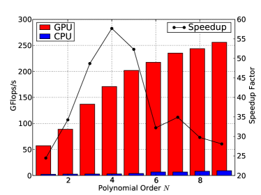
(a) Discontinuous Galerkin performance in GFlops/s on a GPU and a CPU. Computations were performed in single precision.

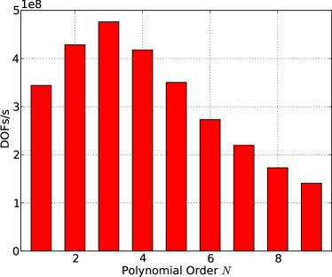
(b) Number of degrees of freedom to which our methods can apply the Maxwelll operator in one second. Assuming linear scaling, this graph can be used to determine run times for larger and smaller problems. DOFs from each of the six Maxwell fields are counted separately.

Figure 8: Performance characteristics of DG on Nvidia graphics hardware.

Orders three and four are particularly favorable not only for their appreciable speedups and their moderate time step requirements [24]. They also achieve the peak nodal value throughputs on the GPU as shown in Figure 8(b). Naturally, high-order approximations of solutions to partial differential equations contain much more information per DOF than do solutions obtained via low order methods. This is most apparent in the number of DOFs required to accurately represent one wavelength [12]. Interestingly, we observe that despite lower computational load, the DG methods of orders one and two achieve lower overall throughput than the next higher ones, a likely result of a mismatch with the hardware’s granularities. This crossover between granularity effects and the increase in floating point work with growing $N$ makes DG methods of orders three and four the fastest DG methods on a GPU even on a per-DOF basis.

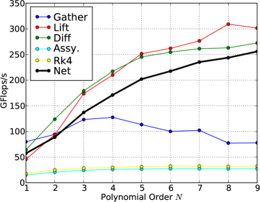
(a) Compute bandwidth in GFlops/s achieved by each part of the DG operator, at various polynomial orders. The published theoretical peak floating point performance for the hardware on which these tests were run is 933 GFlops/s [22].

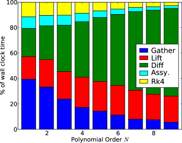
(b) Percentage of time spent in various parts of the DG operator vs. polynomial order.

Figure 9: Performance characteristics of DG on Nvidia graphics hardware, continued.

Recall now that we have split the DG operator into several parts, each of which performs distinct kinds of processing and, as we have seen, tends to require a different strategy to map onto a GPU. It is therefore interesting to see what performance level is attained by each part of the operator. Figure 9(a) gives an indication of this performance, based again on the number of floating point operations per second. It is reassuring that, despite different implementation strategies, the flop rates for element-local differentiation and lifting evolve almost identically as the order $N$ is increased. These two parts of the operator are also characterized by the highest arithmetic intensity and the most regular access pattern. As an unsurprising consequence, they are able to realize the greatest performance gain as the order of the operator and therefore the access granularity grows. The flux gather, on the other hand, realizes its greatest performance at orders three and four. We suspect that the decline in performance with increasing $N$ can be attributed to the growth of the indirect indexing information in the form of face index lists $\mathtt{J}^{\mathtt{T}}$ from Algorithm 3. These lists are referenced constantly throughout the whole algorithm and are therefore likely to reside in the texture cache, of which there are only a few KiB per multiprocessor. As these lists grow, their cache eviction likelihood also grows, resulting in an increased access latency. In addition to the above-mentioned main parts of the operator, the figure also shows performance data for the assembly of the operator and the fourth-order low-storage Runge Kutta timestepper [3]. Both of these operations perform linear combinations of vectors, making them much less arithmetically intense than the element-local operations. Fortunately, as the order $N$ increases, the processing time spent in element-local operations dominates and helps decrease the influence of the latter three operations on overall performance. Figure 9(b) reinforces this point.

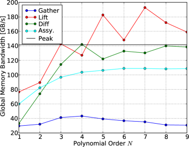
(a) Memory bandwidths in GB/s achieved by each part of the DG operator. The peak memory bandwidth published by the manufacturer is 141.7 GB/s. Values exceeding peak bandwidth are believed to be due to the presence of a texture cache.

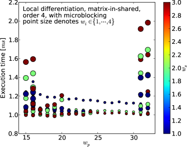
(b) Sample work distribution parameter study for local differentiation on fourth-order elements with microblocking enabled.

Figure 10: Performance characteristics of DG on Nvidia graphics hardware, continued.

It is interesting to correlate the achieved floating point bandwidth of each component from Figure 9(a) with the bandwidth reached for transfers between the processing core and global memory, shown in Figure 10(a). We obtained these numbers by counting the number of bytes fetched from global memory either directly or through a texture unit. The theoretical peak memory bandwidth published by Nvidia is 141.7 GB/s, shown as a black horizontal line. Perhaps the most striking feature at first is the fact that the memory bandwidth measured for flux lifting transcends this theoretical peak at orders five and above. We attribute this phenomenon to the presence of various levels of texture cache. It should perhaps be sobering that the other parts of the DG operator do not manage the same feat. In any case, flux lifting uses the fields-in-shared strategy, and therefore fetches and re-fetches the rather small matrix $L$, making large amounts of data reuse a plausible proposition. Aside from this surprising behavior of flux lifting, it is both interesting and encouraging to see how close to peak the memory bandwidth for element-local differentiation gets. As a converse to the above, this makes it likely that the operation does not get much use out of the texture cache. It does imply, however, that rather impressive work was done by Nvidia’s hardware designers: The theoretical peak global memory bandwidth can very nearly be attained in real-world computations. Next, taking into account what was said in Section 5.2 about the flux-gather part of the operator, the rather low memory throughput achieved is not too surprising–the access pattern is (and, for a general grid, has to be) rather scattered, decreasing the achievable bandwidth. Lastly, operator assembly, which computes linear combination of vectors, consists mainly of global memory fetches and stores. There is no reason why it should be unable to pin the memory subsystem to its peak throughput. Unfortunately, we found ourselves unable to achieve this through loop unrolling or other techniques.

Table 3: Empirically optimal method parameters for each part of the DG operator at polynomial orders 1 through 9.

For potential implementers, it may be interesting to know which exact parameters were used to obtain the results in this section. The parameters of interest include the generic work distribution tuple $(w_{p},w_{i},w_{s})$ for each subtask, the microblock size $K_{M}$, the gather block size $M_{B}$, and which of the matrix- or field-in-shared approaches was used at what order. Table 6 presents this data. It is peculiar how little regularity there is in this data set. Despite a sequence of attempts, we failed to come up with a heuristic that would predict performance accurately. This led us to develop an empirical optimization procedure that finds the data of Table 6 in an automated fashion through a sequence of synthetic and real-world benchmarks. A detailed study of this and other optimization procedures as well as of the toolkit we constructed to enable them will be the subject of a forthcoming report. For now, we restrict ourselves to displaying the results of one such procedure. Figure 10(b) displays the run time obtained for element-local differentiation employing microblocking and the matrix-in-shared strategy at order $N=4$. The objective is to find the work distribution parameter tuple $(w_{p},w_{i},w_{s})$ that leads to an empirically short run time for this part of the operator. It should be stressed that all runs depicted in the figure perform the same amount of work. From Table 6 we see that in this particular instance, an optimum was found at $(w_{p},w_{i},w_{s})=(19,2,3)$. Undoubtedly, with better knowledge of the hardware, many of the odd-looking ups and downs in Figure 10(b) could be understood. Given the published documentation however, we are mostly left to take the results at face value. Luckily, if one were to randomly choose a configuration from the portrayed set, in all likelihood the resulting operation would at most take about 20 per cent longer than the optimal one chosen here. On the other hand, with some bad luck one may also encounter a configuration that makes the computation take about twice as long.

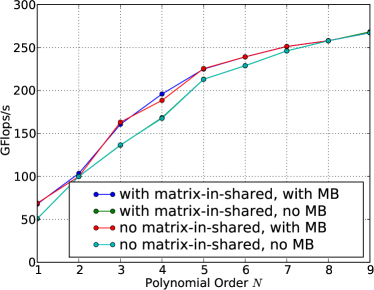
(a) Performance in GFlops/s achieved at various polynomial orders, for different simplified implementations of DG on CUDA.

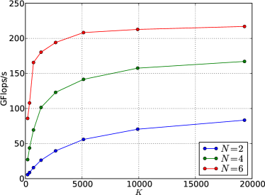
(b) Mesh-dependent scaling of discontinuous Galerkin on Nvidia GPUs.

Figure 11: Performance characteristics of DG on Nvidia graphics hardware, continued.

From Table 6 we can also gather that the field-in-shared strategy with a wide variety of work distribution parameters is found to deliver the best performance at all orders for flux lifting, as well as for higher-order element-local differentiation. This is plausible behavior and was already discussed in Section 5.4. It is therefore reasonable to ask what would be lost if the matrix-in-shared approach were omitted from a GPU DG implementation entirely. Also, we have seen in a number of sections that the introduction of microblocks into the method brings about some mild complications, particularly in the form of shared memory bank conflicts, so one may be compelled to ask how much is lost by ignoring microblocks and simply padding each element to the nearest alignment boundary. The remaining performance after restricting our implementation to not use one or both of these optimizations can be seen in Figure 11(a). Examination of this figure leads to the conclusion that the work of implementing a matrix-in-shared strategy is likely only worthwhile if one is particularly interested in running GPU-DG at a few specific low orders. The benefit of employing mircoblocking, on the other hand, is pervasive and fairly substantial. It stretches to far higher orders than one might suspect at first, given the growth of the involved operands.

Note that these conclusions apply only to the algorithms exactly as described so far. If even one simple trick is omitted from an implementation, tradeoffs may shift dramatically. For example, omitting the thread ordering trick from Section 5.2 makes a matrix-in-shared strategy optimal for differentiation up to order six.

Finally, we note that the performance results in this section depend on the size of the problem being worked on. A very small problem may, for example, not offer enough opportunity to properly occupy all the processing cores that the hardware provides. Figure 11(b) reveals that even relatively small problems achieve decent performance. In addition, we observe that this scaling effect is apparently not just governed by the number of elements present, but also by the order $N$, which influences the number of flops per DOF in the method. We conclude that as soon as there is a certain amount of floating point work to be done per timestep, the method will perform fine.

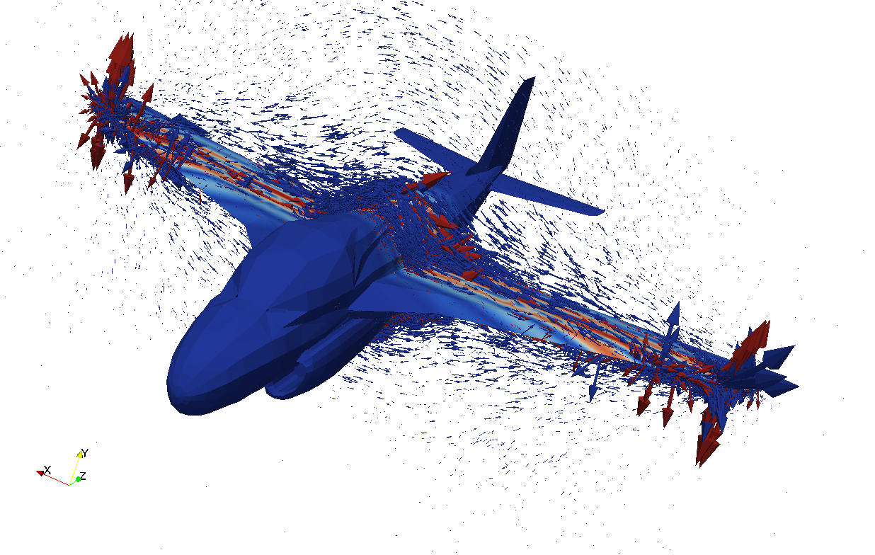
Figure 12: A sample scattering problem solved using the methods described in the text. The incident plane-wave electric field is shown as pseudocolor values on the scatterer, while the scattered electric field is shown as arrows. The computation was performed at order $N=4$ on a mesh of $K=78745$ elements using an incident-field formulation [10] and characteristic absorbing boundary conditions. It achieved and sustained more than 160 GFlops/s.

7 Conclusions

In this paper, we have described and evaluated a variety of techniques for performing discontinuous Galerkin simulations on recent Nvidia graphics processors. We have adapted a number of pre-existing DG codes for the GPU, enabling a thorough comparison of strategies for mapping the method onto the hardware. A final code was written that combines the insights gained from its precursors. This code implements the strategies of Sections 4 and 5 and was used to obtain the results in Section 6.

We have shown that, using our strategies, high-order DG methods can reach double-digit percentages of published theoretical peak performance values for the hardware under consideration. DG computations on GPUs see speed-up factors just short of two orders of magnitude. This speed increase translates directly into an increase of the size of the problem that can be treated using these methods. A single compute device can now do work that previously required a roomful of computing hardware. Alternatively, a cluster of machines equipped with these cards can run simulations that were previously outside the reach of all but the largest supercomputers. This lets the size and complexity of simulations that researchers can afford on a given hardware budget jump significantly.

To make these speed gains accessible, we have provided detailed advice for potential implementers who need to achieve a trade-off between computing performance and implementation effort. The data provided in Section 6 will help them make informed implementation decisions by allowing them to predict the computational speed achieved by their implementations.

We will be extending this work to make use of double precision floating point support that has become available on recent Nvidia hardware. In addition, we would like to broaden the applicability of our methods by exploring their use for nonlinear conservation laws as well as elliptic problems.

Many-core computing presents a rare opportunity, and we feel that discontinuous Galerkin methods have a number of unique characteristics that make them unusually suitable for many-core platforms. In the past, users have chosen low-order methods because of the perceived expense involved in running simulations at a high order of accuracy. While this perception was questionable even in the past, we feel that many-core architectures disproportionately favor high order and significantly drive down its relative cost. Moreover, unlike most other numerical schemes for solving partial differential equations, DG methods make the order of accuracy a tunable parameter. These factors combine to give the user a maximum of control over both performance and accuracy.

7.1 Acknowledgments

The authors gratefully acknowledge the support of AFOSR under grant number FA9550-05-1-0473. The opinions expressed are the views of the authors. They do not necessarily reflect the official position of the funding agencies.

We would like to thank Nvidia Corporation, who, upon completion of this work, provided us with a generous hardware donation for further research.

We would also like to thank Nico Gödel, Akil Narayan, and Lucas Wilcox who provided helpful insights in numerous discussions.

Meshes used in this work were generated using TetGen [20]. The surface mesh for Figure 12 originates in the FlightGear flight simulator and was processed using Blender and MeshLab, a tool developed with the support of the Epoch European Network of Excellence.

Appendix A Index of Notation

Symbol	Meaning	See
$\lceil x\rceil_{n}$	$x$ rounded up to the nearest multiple of $n$.	5.1
$[a,b\rangle$	The set of integers from the half-open interval $[a,b)$.	5.1
$d$	The number of dimensions.	2
$n$	The number of unknowns in the conservation law (1).	4
$N$	Polynomial degree of the approximation space.	2
$N_{p}$	Number of modes/points in local expansion.	4
$N_{fp}$	Number of facial nodes in reference element.	4
$N_{f}$	Number of faces in the reference element.	4
$k$	Used to refer to element numbers.	2
$K$	Total number of elements.	2
$\mathsf{D}_{k}$	The $k$th finite element.	2
$\mathsf{I}$	The unit finite element.	2.1
$\Psi_{k}$	The local-to-global map for element $k$.	2.1
$M^{k}$, $M^{k,A}$, $L^{k}$	Global mass, face mass and lifting matrices for element $k$.	2
$S^{k,\partial\nu}$, $D^{k,\partial\nu}$	$\nu$th global stiffness and differentiation matrices.	2
$M$, $M^{A}$, $L$	Reference mass, face mass and lifting matrices.	2.1
$S^{\partial\mu}$, $D^{\partial\mu}$	$\mu$th reference stiffness and differentiation matrices.	2.1
$\nu$	Used to index global derivatives.	2.1
$\mu$	Used to index local derivatives.	2.1
$T$	Thread scheduling (“warp”) granularity.	3
$K_{M}$	Number of elements in one microblock.	4
$N_{pM}$	Number of volume DOFs in a microblock after padding.	4
$N_{fM}$	Number of face DOFs in a microblock after padding.	5.2
$M_{B}$	Number of microblocks in one flux-gather block.	5.3
$n_{M}$	Total number of microblocks. ($=\lceil K/K_{M}\rceil$)	4
$N_{R}$	Row count of a matrix segment.	5.4
$w_{p}$	The number of work units one block processes in parallel, in different threads.	4
$w_{i}$	The number of work units one block processes inline, in the same thread.	4
$w_{s}$	The number of work units one block processes sequentially, in the same thread.	4
$t_{x},t_{y},t_{z}$	Thread indices in a thread block.	3
$b_{x},b_{y}$	Block indices in an execution grid.	3

References

- Barth and Knight [2005] Timothy Barth and Timothy Knight. A Streaming Language Implementation of the Discontinuous Galerkin Method. Technical Report 20050184165, NASA Ames Research Center, 2005.
- Buck et al. [2004] I. Buck, T. Foley, D. Horn, J. Sugerman, K. Fatahalian, M. Houston, and P. Hanrahan. Brook for GPUs: stream computing on graphics hardware. In Int. Conf. on Computer Graphics and Interactive Techniques, pages 777–786. ACM New York, NY, USA, 2004.
- Carpenter and Kennedy [1994] M. H. Carpenter and C. A. Kennedy. Fourth-order 2N-storage Runge-Kutta schemes. Technical report, NASA Langley Research Center, 1994.
- Cockburn et al. [1990] B. Cockburn, S. Hou, and C. W. Shu. The Runge-Kutta Local Projection Discontinuous Galerkin Finite Element Method for Conservation Laws. IV: The Multidimensional Case. Math. Comp., 54:545–581, 1990.
- Commission [2000] International Electrotechnical Commission. Letter symbols to be used in electrical technology - Part 2: Telecommunications and electronics. Technical report, International Electrotechnical Commission, Geneva, Switzerland, November 2000.
- Dally et al. [2003] W. J. Dally, P. Hanrahan, M. Erez, T. J. Knight, F. Labonté, J. H. Ahn, N. Jayasena, U. J. Kapasi, A. Das, and J. Gummaraju. Merrimac: Supercomputing with streams. In Proceedings of the ACM/IEEE SC2003 Conference (SC’03), volume 1, 2003.
- Göddeke et al. [2005] D. Göddeke, R. Strzodka, and S. Turek. Accelerating double precision FEM simulations with GPUs. In Proceedings of ASIM, 2005.
- Group [2008] Khronos OpenCL Working Group. The OpenCL 1.0 Specification. Khronos Group, December 2008.
- Gumerov and Duraiswami [2008] Nail A. Gumerov and Ramani Duraiswami. Fast multipole methods on graphics processors. J. Comp. Phys., 227:8290–8313, September 2008. doi: 10.1016/j.jcp.2008.05.023.
- Hesthaven and Warburton [2002] J. S. Hesthaven and T. Warburton. Nodal High-Order Methods on Unstructured Grids: I. Time-Domain Solution of Maxwell’s Equations. J. Comp. Phys., 181:186–221, September 2002. doi: 10.1006/jcph.2002.7118.
- Hesthaven and Warburton [2007] J. S. Hesthaven and T. Warburton. Nodal Discontinuous Galerkin Methods: Algorithms, Analysis, and Applications. Springer, first edition, November 2007. ISBN 0387720650.
- Hesthaven et al. [2007] J. S. Hesthaven, S. Gottlieb, and D. Gottlieb. Spectral Methods for Time-Dependent Problems. Cambridge University Press, 2007. ISBN 0521792118.
- Jackson [1998] J. D. Jackson. Classical Electrodynamics. Wiley, third edition, July 1998. ISBN 047130932X.
- Karypis and Kumar [1999] G. Karypis and V. Kumar. A Fast and High Quality Multilevel Scheme for Partitioning Irregular Graphs. SIAM J. Sci. Comp., 20:359–392, 1999.
- Krakiwsky et al. [2004] S.E. Krakiwsky, L.E. Turner, and M.M. Okoniewski. Acceleration of finite-difference time-domain (FDTD) using graphics processor units (GPU). In Microwave Symposium Digest, 2004 IEEE MTT-S International, volume 2, pages 1033–1036 Vol.2, 2004. ISBN 0149-645X. doi: 10.1109/MWSYM.2004.1339160.
- Li et al. [2003] W. Li, X. Wei, and A. Kaufman. Implementing Lattice Boltzmann computation on graphics hardware. The Visual Computer, 19:444–456, 2003.
- Lindholm et al. [2008] E. Lindholm, J. Nickolls, S. Oberman, and J. Montrym. Nvidia Tesla: A Unified Graphics and Computing Architecture. Micro, IEEE, 28:39–55, 2008. ISSN 0272-1732. doi: 10.1109/MM.2008.31.
- Nvidia Corporation [2008] Nvidia Corporation. NVIDIA CUDA 2.0 Compute Unified Device Architecture Programming Guide. Nvidia Corporation, Santa Clara, USA, June 2008.
- Reed and Hill [1973] W. H. Reed and T. R. Hill. Triangular mesh methods for the neutron transport equation. Technical report, Los Alamos Scientific Laboratory, Los Alamos, 1973.
- Si and Gaertner [2005] H. Si and K. Gaertner. Meshing Piecewise Linear Complexes by Constrained Delaunay Tetrahedralizations. In Proc. of the 14th International Meshing Roundtable, pages 147–163. Springer, 2005.
- Stratton et al. [2008] J. Stratton, S. Stone, and W. Hwu. MCUDA: An Efficient Implementation of CUDA Kernels on Multi-cores. Technical report, University of Illinois at Urbana-Champaign, Urbana-Champaign, IL, USA, March 2008.
- Various authors [2008] Various authors. Comparison of Nvidia graphics processing units — Wikipedia, The Free Encyclopedia, 2008. URL http://en.wikipedia.org/w/index.php?title=Comparison_of_Nvidia_graphics%_processing_units&oldid=248858931. [Online; accessed 9-November-2008].
- Warburton [2006] T. Warburton. An explicit construction of interpolation nodes on the simplex. J. Eng. Math., 56:247–262, 2006.
- Warburton and Hagstrom [2008] T. Warburton and T. Hagstrom. Taming the CFL Number for Discontinuous Galerkin Methods on Structured Meshes. SIAM J. Num. Anal., 46:3151–3180, 2008. doi: 10.1137/060672601.
- Whaley et al. [2001] R. C. Whaley, A. Petitet, and J. J. Dongarra. Automated empirical optimizations of software and the ATLAS project. Parallel Computing, 27:3–35, 2001.