KEK-TH-1296 December 2008

Vertex operators of Type IIB matrix model
via calculation of disk amplitudes

Yoshihisa Kitazawa^1),2) and Toshikazu Negi²⁾

¹⁾ High Energy Accelerator Research Organization (KEK),

Tsukuba, Ibaraki 305-0801, Japan

²⁾ Department of Particle and Nuclear Physics,

The Graduate University for Advanced Studies (SOKENDAI),

Tsukuba, Ibaraki 305-0801, Japan

We investigate the vertex operators of the supergravity multiplet in IIB(IKKT) matrix model by calculating the disk amplitudes, exploiting the technique of conformal field theory. The vertex operators of IIB matrix model are given as the coupling of a closed string and the open strings which are introduced by the existence of D($-1$)-branes. We consider the most generic couplings which involve both the bosonic and fermionic open strings. Our results are consistent with the previous results based on supersymmetry. We thus confirm the structure of the IIB matrix model vertex operators from the first principle.

1 Introduction

Type IIB (IKKT) matrix model [1] is one of the proposal to define the superstring theory nonperturbatively. It is formulated as the zero-dimensional reduced model of the maximally supersymmetric Yang-Mills theory. In the case of finite matrix size $N$, it can be thought as the effective theory of D-instantons.

Action of the type IIB matrix model is :

$$S=-\frac{1}{g^{2}}Tr\left[\frac{1}{4}[A_{\mu},A_{\nu}][A^{\mu},A^{\nu}]+\frac{1}{2}\bar{\epsilon}\gamma^{\mu}[A_{\mu},\epsilon]\right],$$ (1.1)

where $A_{\mu}$ and $\epsilon$ are $N\times N$ Hermitian matrices. $A_{\mu}$ is a ten-dimensional vector and $\epsilon$ is a ten-dimensional Majorana-Weyl spinor field respectively.

To calculate the correlators in type IIB matrix model, it is necessary to construct the vertex operators. Their bosonic terms are determined first by one of the authors [2] by exploiting supersymmetry. Subsequently a systematic procedure is developed through the construction of the supersymmetric Wilson loop operator. In this way, the vertex operator is determined completely up to the 4-th rank antisymmetric tensor [3, 4]. Recently there was a further progress in determining the precise form of vertex operators for the matrix model [5].

In this paper, we investigate the vertex operators by using conformal field theoretical technique. In this method, the bosonic part of the vertex operators is investigated in [2, 6, 7] in the presence of $N$ D(-1)-branes. The investigation of the fermionic part is carried out in [9] for the case of a single D(-1)-brane. We extend these investigations into the most generic case. Namely, we consider both the fermionic and bosonic open strings in the presence of $N$ D(-1)-branes. In the case of a single D(-1)-brane [9], the Majorana-Weyl fermions were not matrices. In the presence of $N$ D(-1)-branes, Majorana-Weyl fermions become $N\times N$ matrices. The matrix model vertex operator becomes the Wilson lines due to the multiple insertions of the bosonic open string vertex operators. Type IIB superstring theory is a closed string theory. The type IIB matrix model is multiple D(-1)-brane theory for finite $N$. The existence of the D-branes introduces open strings. The disk amplitude technique relies on the fact that the the vertex operator couples the closed strings to open strings. Disk amplitude technique was also used in the study of supersymmetric four-dimensional effective gauge theories with instantons from type IIB superstring theory such as in [15].

In comparison to the previous investigations using supersymmetric transformation in IIB matrix model [3, 4, 5], we can check that the resultant formulae give the consistent form of the vertex operators for the IIB matrix model up to the 4-th rank antisymmetric tensor completely.

This paper is organized as follows. In section 2, we introduce the disk amplitudes which couple closed strings in the bulk to open strings on the boundary. In section 3, we define the conformal field theory vertex operators that are necessary to calculate the disk amplitude. From the section 4 to section 9, we investigate the explicit structure of the vertex operators of the type IIB matrix model via the calculation of the disk amplitudes. We conclude in section 10 with discussions.

2 Disk amplitudes

In this section, we introduce the disk amplitudes which couple closed strings in the bulk to open strings on the boundary. They will be investigated in the subsequent sections.

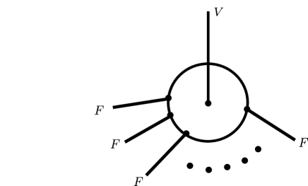
When there exist D-branes, they introduce the boundary to the string world-sheet. So the topology of the world-sheet becomes a disk and it is conformaly equivalent to the upper half plane. We put open string vertex operator on the boundary of the disk, namely the real axis. We put a closed string vertex operator in the inner part of the disk, i.e. at a location $z$ in the upper half plane. The closed string vertex operator, bosonic and fermionic open string vertex operator are denoted as $V$, $U$ and $F$ respectively. The concrete form of the $V$, $U$ and $F$ are given in the next section. We illustrate the disk amplitude in Figure.2.1.

We focus on the supergravity multiplet in type IIB superstring theory. They are the BPS states which preserve the half SUSY (16 supercharges). The IIB supergravity multiplet consists of a complex dilaton $\mathbf{\Phi}$, a complex dilatino $\Lambda$, a complex antisymmetric tensor $B_{\mu\nu}$, a complex gravitino $\mathbf{\Psi}_{\mu}$, a real graviton $h_{\mu\nu}$ and a real 4-th rank antisymmetric tensor $A_{\mu\nu\rho\sigma}$. They are generated from the complex dilaton by acting 16 broken SUSY generators. By regarding the complex dilaton as the highest state in the supergravity multiplet, we can classify the type IIB supergravity multiplet as Table.2.1.

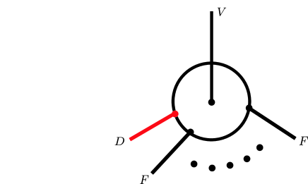
For the vertex operator $V$ at the $n$-th SUSY level, we may put $n$ fermionic open strings on the boundary of the world-sheet. We may also put $m$ bosonic strings and $n-2m$ fermionic open strings (where $2m\leq n$). For example we can insert a single bosonic open string vertex operator on the boundary instead of $2$ fermionic open strings. Such an amplitude is illustrated in Figure.2.2.

Table 2.1: Massless multiplet of the type IIB superstring theory.

SUSY($n$-th level)	type IIB supergravity multiplet
$n=0$	complex scalar $\mathbf{\Phi}$ ((NS-NS dilaton) + (R-R axion))
$n=1$	complex dilatino $\Lambda$
$n=2$	complex antisymmetric tensor $B_{\mu\nu}$
$n=3$	complex gravitino $\mathbf{\Psi_{\mu}}$
$n=4$	real graviton $h_{\mu\nu}$ and real 4-th rank antisymmetric tensor $A_{\mu\nu\rho\sigma}$

Figure 2.1: Disk amplitude in which $n$-th SUSY level closed string vertex operator couples to $n$ open strings.$V$ denotes the closed string (supergravity) vertex operator. $F$ denotes the vertex operator of the fermionic open string.

Figure 2.2: Alternative to $n$ fermionic open strings, the closed string vertex operator can couple to $n-2$ fermionic open strings and a single bosonic open string.

3 Vertex operators

The vertex operator of the closed string that satisfies the NS-NS boundary condition is

$$V^{\mathrm{NN}}_{(-1,-1)}(z,\bar{z})=\zeta^{\mathrm{NN}}_{\mu\nu}\psi^{\mu}(z)e^{-\phi(z)}\bar{\psi}^{\nu}(\bar{z})e^{-\bar{\phi}(\bar{z})}e^{ikX(z,\bar{z})},$$ (3.2)

If $\zeta^{\mathrm{NN}}_{\mu\nu}$ is a traceless symmetric tensor, it corresponds to the vertex operator for the graviton. In the case of $(0)$-picture, instead of $e^{-\phi(z)}\psi(z)$, we use $\partial X^{\mu}(z)+ik_{\rho}j^{\mu\rho}(z)$. For instance, $V^{\text{NN}}_{(0,-1)}(z,\bar{z})$ becomes as follows,

$$V^{\mathrm{NN}}_{(0,-1)}(z,\bar{z})=\zeta^{\mathrm{NN}}_{\mu\nu}(\partial X^{\mu}(z)+ik_{\rho}j^{\mu\rho}(z))\bar{\psi}(\bar{z})e^{-\bar{\phi}(\bar{z})}e^{ikX(z,\bar{z})}.$$ (3.3)

The R-R vertex operator involves the spin field $S$. For example,

$$V^{\mathrm{RR}}_{(-\frac{1}{2},-\frac{1}{2})}(z,\bar{z})=\zeta^{\mathrm{RR}}_{\mu\nu}S^{a}(z)e^{-\frac{1}{2}\phi(z)}(\gamma^{\mu\nu})_{ab}\bar{S}^{b}(\bar{z})e^{-\frac{1}{2}\bar{\phi}(\bar{z})}e^{ikX(z,\bar{z})}.$$ (3.4)

is the vertex operator for the second rank antisymmetric tensor.

When D$(-1)$ -branes exist, we need to introduce open string vertex operators in this theory. The bosonic one is

$$U_{0}(t)= \Phi^{\mu}(X)ig_{\mu\nu}\partial_{\perp}X^{\nu}(t)-ig_{\mu\rho}g_{\nu\sigma}[\Phi^{\rho}(X),\Phi^{\sigma}(X)]\Psi^{\mu}\Psi^{\nu}(t)$$

$$\equiv W^{(0)}(t)+D^{(0)}(t),$$ (3.5)

where $\Phi^{\mu}$ is the bosonic field and it is related to $A^{\mu}$ (the bosonic degree of freedom in the type IIB matrix model) by

$$2\pi\alpha^{\prime}\Phi^{\mu}=A^{\mu},$$ (3.6)

where we put

$$\alpha^{\prime}=1$$ (3.7)

in our convention. We have decomposed $U^{(0)}$ into the two vertex operators $W^{(0)}$ and $D^{(0)}$.

$$W^{(0)}(t)=\Phi^{\mu}(X)ig_{\mu\nu}\partial_{\perp}X^{\nu}(t),$$

$$D^{(0)}(t)=-ig_{\mu\rho}g_{\nu\sigma}[\Phi^{\rho}(X),\Phi^{\sigma}(X)]\Psi^{\mu}\Psi^{\nu}(t).$$ (3.8)

This vertex operator is introduced in [6, 7]. Here we introduce $\Psi(t)$ as the fermionic field on the boundary. The exponentiated term of $W^{(0)}$, namely $\exp(iW^{(0)})$ always appears in our calculation and introduces the Wilson-line structure in the matrix model vertex operators. The fermionic open string vertex operators are

$$F_{-\frac{1}{2}}(x)=\epsilon_{a}S^{a}(x)e^{-\frac{1}{2}\phi(x)}$$ (3.9)

and

$$F_{\frac{1}{2}}(x)=\epsilon^{a}(\gamma_{\mu})_{ab}S^{b}(x)\partial_{\perp}X^{\mu}(x)e^{\frac{1}{2}\phi(x)},$$ (3.10)

where $\epsilon$’s are the Majorana-Weyl spinors. These vertex operators are considered in [9] for a single D instanton. In this paper, we generalize them for $N$ D$(-1)$-branes. Therefore $A$ and $\epsilon$ become $N\times N$ matrices. In this process, we also introduce the vertex operator that contains the commutator of $A$ and $\epsilon$. Because the conformal weight of the operator $\Psi^{\alpha}\Psi^{\beta}(x)$ is the same with $\partial_{\mu}$, we can add the following operator to (3.10):

$$C_{+\frac{1}{2}}(x)=[\epsilon_{a},\Phi_{\alpha}](\gamma_{\beta})^{ab}\Psi^{\alpha}\Psi^{\beta}(x)S^{b}(x)e^{+\frac{1}{2}\phi(x)}.$$ (3.11)

This operator contains a bosonic string and a fermionic string. Thus we can substitute this operator for $3$ fermionic strings. Using these operators, we calculate the disk amplitudes exploiting conformal field theory technique[8].

$W^{(0)}$, $F_{\frac{1}{2}}$, $D^{(0)}$ and $C_{\frac{1}{2}}$ contains the fields of type IIB matrix model as follows:

$$W^{(0)}\propto A,$$

$$F_{\frac{1}{2}}\propto\epsilon,$$

$$D^{(0)}\propto[A,A],$$

$$C_{\frac{1}{2}}\propto[\epsilon,A].$$ (3.12)

Just like the closed string vertex operators in Table.2.1 , we can classify the open string vertex operators by their SUSY level. Namely, starting with $W^{(0)}$, we can assign a SUSY level to each operator as in Table.3.2.

Table 3.2: Open string vertex operators and fields.

Vertex operator	Field in type IIB matrix model	SUSY($n$-th level)
$W^{(0)}$	$A$	$0$
$F_{\frac{1}{2}}$	$\epsilon$	$1$
$D^{(0)}$	$[A,A]$	$2$
$C_{\frac{1}{2}}$	$[A,\epsilon]$	$3$

We calculate the disk amplitude in which $V$ is in the upper half plane and a group of open string vertex operators consisting of $W^{(0)}$, $F_{\frac{1}{2}}$, $D^{(0)}$, $C_{\frac{1}{2}}$ are on the boundary. In order to respect space-time SUSY in our calculation, we impose the following condition for a group of the open string vertex operators; i.e. ”SUSY level of a closed string vertex operator $V$ (shown in Table.2.1) should be equal to the total SUSY level of a group of the open string vertex operators on the boundary (shown in 3.2)”. Because we set the level of $W^{(0)}$ as $0$, the closed string vertex operator $V$ always can couple to infinite number of $W^{(0)}$’s. In fact $V$ always couples to

$$\exp(iW^{(0)}),$$ (3.13)

which corresponds to the Wilson-line operator in the matrix model.

In type IIB matrix model, the highest state in the SUSY classification is a complex scalar. In Table.3.2, we have assigned it null SUSY level. Thus this field can couple only to $\exp(iW^{(0)})$. The SUSY level for dilatino is $1$. So the dilatino field can couple to $\exp(iW^{(0)})$ and one fermionic open string. Since the SUSY level for B-field is $2$, it can couple two $F_{\frac{1}{2}}$ or one $D^{(0)}$ in addition to $\exp(iW^{(0)})$. We can calculate other disk amplitudes in a similar way. With this rule, we will demonstrate that the precise form of the vertex operators in type IIB matrix model can be reproduced from conformal field theory.

3.1 Propagators

In order to calculate the disk amplitudes, we need the two point functions for $X$’s and $\psi$’s. The two point function for $X$’s is given as :

$$\langle X^{\mu}(z)X^{\nu}(w)\rangle=-\left(g^{\mu\nu}\ln|z-w|-g^{\mu\nu}\ln|z-\bar{w}|+2G^{\mu\nu}\ln|z-\bar{w}|\right),$$ (3.14)

where $g^{\mu\nu}$ is a closed string metric and $G^{\mu\nu}$ is an open string metric. Here for the open string metric, we take

$$G^{\mu\nu}=0.$$ (3.15)

We consider $g_{\mu\nu}$ as Minkowski spacetime metric :

$$g_{\mu\nu}=diag(-1,+1,+1,\dots,+1).$$ (3.16)

So

$$\langle X^{\mu}(z)X^{\nu}(w)\rangle=-g^{\mu\nu}\ln\left|\frac{z-t}{\bar{z}-t}\right|.$$ (3.17)

For later conveniences, we introduce a function $\tau(t,z)$ as

$$\tau(t,z)=\frac{1}{2\pi i}\ln\left(\frac{t-z}{t-\bar{z}}\right).$$ (3.18)

It is related to the Dirichlet propagator as

$$i\partial_{\perp}\left[\ln\left|\frac{z-t}{\bar{z}-t}\right|\right]=\frac{z-\bar{z}}{(z-t)(\bar{z}-t)}=2\pi i\frac{\partial\tau(t,z)}{\partial t}.$$ (3.19)

For a fixed value of $z$, $\tau(t,z)$ is a monotonically increasing function of $t$ and

$$\tau(\infty,z)-\tau(-\infty,z)=1.$$ (3.20)

Next we write down the $2$-point functions of fermions,

$$\langle\psi^{\mu}(z)\psi^{\nu}(w)\rangle=\frac{1}{z-w}g^{\mu\nu},$$

$$\langle\psi^{\mu}(z)\psi^{\nu}(\bar{w})\rangle=\frac{1}{z-\bar{w}}\left(-g^{\mu\nu}+2G^{\mu\nu}\right),$$

$$\langle\bar{\psi}^{\mu}(\bar{z})\psi^{\nu}(w)\rangle=\frac{1}{\bar{z}-w}(-g^{\mu\nu}+2G^{\mu\nu}),$$

$$\langle\bar{\psi}^{\mu}(z)\bar{\psi}^{\nu}(\bar{w})\rangle=\frac{1}{\bar{z}-\bar{w}}g^{\mu\nu}.$$ (3.21)

The boundary-boundary and bulk-boundary propagators for the fermions are given by

$$\langle\Psi^{\mu}(t)\Psi^{\nu}(t^{\prime})\rangle=\frac{1}{t-t^{\prime}}g^{\mu\nu},$$

$$\langle\psi^{\mu}(z)\Psi^{\nu}(t)\rangle=\frac{1}{z-t}g^{\mu\nu},$$

$$\langle\bar{\psi}^{\mu}(\bar{z})\Psi^{\nu}(t)\rangle=-\frac{1}{\bar{z}-t}g^{\mu\nu}.$$ (3.22)

4 Scalar field

Having set up the disk amplitude calculation which involves closed string vertex operators in the bulk and open string vertex operators on the boundary, we start explicit evaluations of these amplitudes in conformal field theory. We start with the simplest case, namely the complex scalar which is the highest state in the SUSY classification. In type IIB supergravity multiplet, there are two kinds of Lorentz scalars. They are dilaton and axion, which satisfy the NS-NS and R-R boundary condition, respectively. Here we need the disk amplitude for complex scalar. Therefore the amplitude that we want to consider is the complex combination of the NS-NS part and R-R part and it becomes as follows :

$$\langle\mathbf{\Phi}\rangle=\langle\mathbf{\Phi}^{\mathrm{NN}}\rangle+i\langle\mathbf{\Phi}^{\mathrm{RR}}\rangle.$$ (4.23)

Scalar field can couple only to bosonic open strings that results in the Wilson line; i.e. the term given as follows :

$$W^{(0)}(t_{a})=\Phi^{\rho}ig_{\rho\sigma}\partial_{\perp}X^{\sigma}(t_{a}).$$ (4.24)

The disk amplitude for the NS-NS dilation is given as

$$\sum_{n=0}^{\infty}2\pi iTr\mathbf{P}\int_{-\infty}^{+\infty}dt_{2}dt_{3}\dots dt_{n-1}dt_{n}\langle c(z)\bar{c}(\bar{z})c(t_{1})\rangle\langle V^{\mathrm{NN}}_{(-1,-1)}(z,\bar{z})\frac{1}{n!}\prod_{a=1}^{n}\left(iW^{(0)}(t_{a})\right)\rangle$$

$$= \sum_{n=0}^{\infty}2\pi iTr\mathbf{P}\int_{-\infty}^{+\infty}dt_{2}dt_{3}\dots dt_{n-1}dt_{n}(z-\bar{z})(z-t_{1})(\bar{z}-t_{1})$$

$$\times\langle\left[\zeta^{\mathrm{NN}}_{(0)}g_{\mu\nu}\psi^{\mu}(z)e^{-\phi}(z)\bar{\psi}^{\nu}(\bar{z})e^{-\bar{\phi}}(\bar{z})e^{ikX(z,\bar{z})}\right]\prod_{a=1}^{n}\frac{1}{n!}\left(i\Phi^{\rho}ig_{\rho\sigma}\partial_{\perp}X^{\sigma}(t_{a})\right)\rangle$$

$$= \sum_{n=0}^{\infty}2\pi iTr\mathbf{P}\int_{-\infty}^{+\infty}dt_{2}dt_{3}\dots dt_{n-1}dt_{n}(z-\bar{z})(z-t_{1})(\bar{z}-t_{1})$$

$$\times\zeta^{\mathrm{NN}}_{(0)}\frac{-g_{\mu\nu}g^{\mu\nu}}{(z-\bar{z})^{2}}\prod_{a=1}^{n}\frac{1}{n!}\left[-\Phi^{\rho}g_{\rho\sigma}[-ik_{\alpha}g^{\alpha\sigma}\partial_{\perp}\ln\left|\frac{z-t_{a}}{\bar{z}-t_{a}}\right|]\right]$$

$$= \sum_{n=0}^{\infty}2\pi iTr\mathbf{P}\frac{1}{n!}\int_{-\infty}^{+\infty}dt_{2}dt_{3}\dots dt_{n-1}dt_{n}$$

$$\times\zeta^{\mathrm{NN}}_{(0)}\left[(z-\bar{z})(z-t_{1})(\bar{z}-t_{1})\frac{-D}{(z-\bar{z})^{2}}\left(\Phi\cdot k\right)\frac{z-\bar{z}}{(z-t_{1})(\bar{z}-t_{1})}\right]$$

$$\times\prod_{a=2}^{n}\left[\left(\Phi\cdot k\right)\frac{z-\bar{z}}{(z-t_{a})(\bar{z}-t_{a})}\right]$$

$$= \sum_{n=0}^{\infty}Tr\mathbf{P}\bigg{[}\frac{1}{n!}\int_{-\infty}^{+\infty}dt_{2}dt_{3}\dots dt_{n-1}dt_{n}$$

$$\times\bigg{\{}-\zeta^{\mathrm{NN}}_{(0)}D\left(2\pi i\Phi\cdot k\right)\prod_{a=2}^{n}\left[(\Phi\cdot k)2\pi i\frac{\partial\tau(t_{a},z)}{\partial t_{a}}\right]\bigg{\}}\bigg{]}$$

$$= -\sum_{n=0}^{\infty}Tr\mathbf{P}D\zeta^{\mathrm{NN}}_{(0)}\prod_{a=1}^{n}\left[\frac{1}{n!}\int^{\infty}_{-\infty}dt_{a}\left[i\left(2\pi\Phi\cdot k\right)\frac{\partial\tau(t_{a},z)}{\partial t_{a}}\right]\right]$$

$$= -D\zeta^{\mathrm{NN}}_{(0)}\sum_{n=0}^{\infty}Tr\mathbf{P}\prod_{a=1}^{n}\frac{1}{n!}\left[\int^{1}_{0}d\tau\left[i\left(A\cdot k\right)\right]\right]$$

$$= -D\zeta^{\mathrm{NN}}_{(0)}STr\exp\left(iA\cdot k\right),$$ (4.25)

where $D$ is the number of spacetime dimensions and in the superstring theory, we consider the case $D=10$. $Tr$ is the trace for $A$ and $\epsilon$ matrices. We use $tr$ for the trace for $\gamma$ - matrices. $STr$ denotes the symmetrized trace defined in Appendix A.4. $\mathbf{P}$ denotes the path-ordered operators. Up to a normalization constant, we find

$$\zeta^{\mathrm{NN}}_{(0)}STr\exp\left(iA\cdot k\right).$$ (4.26)

Secondly, we calculate the disk amplitude for the axion. The amplitude is

$$\sum_{n=0}^{\infty}2\pi iTr\mathbf{P}\int_{-\infty}^{+\infty}dt_{2}dt_{3}\dots dt_{n-1}dt_{n}\langle c(z)\bar{c}(\bar{z})c(t_{1})\rangle\langle V^{\mathrm{RR}}_{(-\frac{1}{2},-\frac{3}{2})}(z,\bar{z})\frac{1}{n!}\prod_{a=1}^{n}\left(iW^{(0)}(t_{a})\right)\rangle$$

$$= \sum_{n=0}^{\infty}2\pi iTr\mathbf{P}\frac{1}{n!}\int_{-\infty}^{+\infty}dt_{2}dt_{3}\dots dt_{n-1}dt_{n}(z-\bar{z})(z-t_{1})(\bar{z}-t_{1})$$

$$\times\langle\left[\zeta^{\mathrm{RR}}_{(0)}e^{-\frac{1}{2}\phi}(z)S^{a}(z)\delta_{ab}S^{b}(\bar{z})e^{-\frac{3}{2}\bar{\phi}}(\bar{z})e^{ikX(z,\bar{z})}\right]\prod_{a=1}^{n}[i\Phi^{\rho}ig_{\rho\sigma}\partial_{\perp}X^{\sigma}(t_{a})]\rangle.$$ (4.27)

The OPE for 2-point function of the spin fields is given by (A.148). So the disk amplitude is

$$\sum_{n=0}^{\infty}\frac{1}{n!}2\pi iTr\mathbf{P}\int_{-\infty}^{+\infty}dt_{2}dt_{3}\dots dt_{n-1}dt_{n}(z-\bar{z})(z-t_{1})(\bar{z}-t_{1})$$

$$\times\zeta^{\mathrm{RR}}_{(0)}\left[\delta_{ab}(z-\bar{z})^{-\frac{3}{4}}\right]\frac{-\delta^{ab}}{(z-\bar{z})^{\frac{5}{4}}}\prod_{a=1}^{n}\left[-\Phi^{\rho}g_{\rho\sigma}[-ik_{\alpha}g^{\alpha\sigma}\partial_{\perp}\ln\left|\frac{z-t_{a}}{\bar{z}-t_{a}}\right|]\right]$$

$$= \sum_{n=0}^{\infty}2\pi iTr\mathbf{P}\frac{1}{n!}\int_{-\infty}^{+\infty}dt_{2}dt_{3}\dots dt_{n-1}dt_{n}$$

$$\times\zeta^{\mathrm{RR}}_{(0)}\left[(z-\bar{z})(z-t_{1})(\bar{z}-t_{1})\frac{-2^{\frac{D}{2}}}{(z-\bar{z})^{2}}\left(\Phi\cdot k\right)\frac{z-\bar{z}}{(z-t_{1})(\bar{z}-t_{1})}\right]$$

$$\times\prod_{a=2}^{n}\left[\left(\Phi\cdot k\right)\frac{z-\bar{z}}{(z-t_{a})(\bar{z}-t_{a})}\right]$$

$$= \sum_{n=0}^{\infty}Tr\mathbf{P}\left[\frac{1}{n!}\int_{-\infty}^{+\infty}dt_{2}dt_{3}\dots dt_{n-1}dt_{n}\zeta^{\mathrm{RR}}_{(0)}(-2^{\frac{D}{2}})\left(2\pi i\Phi\cdot k\right)\prod_{a=2}^{n}\left[(\Phi\cdot k)2\pi i\frac{\partial\tau(t_{a},z)}{\partial t_{a}}\right]\right]$$

$$= -2^{\frac{D}{2}}\zeta^{\mathrm{RR}}_{(0)}\sum_{n=0}^{\infty}Tr\mathbf{P}\prod_{a=1}^{n}\frac{1}{n!}\left[\int dt_{a}\left[i\left(2\pi\Phi\cdot k\right)\frac{\partial\tau(t_{a},z)}{\partial t_{a}}\right]\right]$$

$$= -2^{\frac{D}{2}}\zeta^{\mathrm{RR}}_{(0)}\sum_{n=0}^{\infty}Tr\mathbf{P}\prod_{a=1}^{n}\frac{1}{n!}\left[\int^{1}_{0}d\tau\left[i\left(A\cdot k\right)\right]\right]$$

$$= -2^{\frac{D}{2}}\zeta^{\mathrm{RR}}_{(0)}STr\exp\left(i\left(A\cdot k\right)\right).$$ (4.28)

We thus find the identical result with (4.26),

$$\zeta^{\mathrm{RR}}_{(0)}STr\exp\left(iA\cdot k\right).$$ (4.29)

Therefore, by forming a linear combination (4.26)$+i$(4.29), we can derive the vertex operator for the scalar field in typeIIB matrix model as

$$(\zeta^{\mathrm{NN}}_{(0)}+i\zeta^{\mathrm{RR}}_{(0)})STr\exp\left(ik\cdot A\right)\equiv\mathbf{\Phi}(\lambda)\ V^{\mathbf{\Phi}}(A,\epsilon).$$ (4.30)

5 Dilatino

Next we calculate the disk amplitude for the dilatino. The disk amplitude for the complex dilatino is given as

$$\langle\Lambda\rangle=\langle\Lambda^{\mathrm{RN}}\rangle+i\langle\Lambda^{\mathrm{NR}}\rangle.$$ (5.31)

Dilatino couples to one fermionic open string. Firstly, the disk amplitude for the NS-R dilatino field is

$$\langle\Lambda^{\mathrm{NR}}\rangle$$

$$= \langle c(z)\bar{c}(\bar{z})V^{\mathrm{NR}}_{(-1,-\frac{1}{2})}(z,\bar{z})c(x_{1})Tr\mathbf{P}\exp\left(i\int dtW^{(0)}(t)\right)F_{-\frac{1}{2}}(x_{1})\rangle$$

$$= \langle c(z)c(\bar{z})\zeta^{\mathrm{NR}}_{\mu a}e^{-\phi}(z)\psi^{\mu}(z)\bar{S}^{a}(\bar{z})e^{-\frac{1}{2}\bar{\phi}}(\bar{z})e^{ikX}(z,\bar{z})$$

$$\times Tr\mathbf{P}\exp\left(i\int dt\Phi^{\rho}ig_{\rho\sigma}\partial_{\perp}X^{\sigma}(t)\right)c(x_{1})\epsilon_{b}S^{b}(x_{1})e^{-\frac{1}{2}\phi(x_{1})}\rangle$$

$$= \zeta^{\mathrm{NR}}_{\mu a}Tr\mathbf{P}\exp\left(-\int dt\Phi^{\alpha}(-ik_{\alpha})\partial_{\perp}\ln\left|\frac{z-t}{\bar{z}-t}\right|\right)$$

$$\times\left[(z-\bar{z})(z-x_{1})(\bar{z}-x_{1})\right]\left[(z-\bar{z})^{-\frac{1}{2}}(z-x_{1})^{-\frac{1}{2}}(\bar{z}-x_{1})^{-\frac{1}{4}}\right]$$

$$\times\left[(\gamma^{\mu})^{ab}(z-\bar{z})^{-\frac{1}{2}}(z-x_{1})^{-\frac{1}{2}}(\bar{z}-x_{1})^{-\frac{3}{4}}\right]\epsilon_{b}$$

$$= \zeta^{\mathrm{NR}}_{\mu a}(\gamma^{\mu})^{ab}Tr\mathbf{P}\exp\left(\int dt\Phi^{\alpha}ik_{\alpha}\partial_{\perp}\ln\left|\frac{z-t}{\bar{z}-t}\right|\right)\epsilon_{b}$$

$$= \zeta^{\mathrm{NR}}_{\mu a}(\gamma^{\mu})^{ab}Tr\mathbf{P}\exp\left(i\int dt(2\pi\Phi\cdot k)\frac{\partial\tau}{\partial t}\right)\epsilon_{b}$$

$$= \zeta^{\mathrm{NR}}_{\mu a}(\gamma^{\mu})^{ab}STr\exp\left(ik\cdot A\right)\epsilon_{b},$$ (5.32)

where we used the correlator

$$\langle\psi^{\mu}(z_{1})S^{a}(z_{2})S^{b}(z_{3})\rangle=(z_{1}-z_{2})^{-\frac{1}{2}}(z_{1}-z_{3})^{-\frac{1}{2}}(z_{2}-z_{3})^{-\frac{3}{4}}(\gamma^{\mu})^{ab}.$$ (5.33)

The disk amplitude for the R-NS dilatino field is similarly calculated as

$$\langle\Lambda^{\mathrm{RN}}\rangle$$

$$= \langle c(z)\bar{c}(\bar{z})V^{\mathrm{RN}}(z,\bar{z})c(x_{1})Tr\mathbf{P}\exp\left(i\int dtW^{(0)}(t)\right)F_{-\frac{1}{2}}(x_{1})\rangle$$

$$= -\zeta^{\mathrm{RN}}_{a\mu}STr\left(\exp\left(ik\cdot A\right)(\gamma^{\mu})^{ab}\epsilon_{b}\right).$$ (5.34)

From (5.34)$+i$(5.32), we get

$$(\zeta^{\mathrm{RN}}_{\mu a}+i\zeta^{\mathrm{NR}}_{a\mu})(\gamma^{\mu})^{ab}STr\left(e^{ik\cdot A}\epsilon_{b}\right)\equiv\Lambda(\lambda)V^{\Lambda}(A,\epsilon),$$ (5.35)

where $\Lambda(\lambda)$ is the wave function of dilatino and it is defined as

$$\Lambda^{b}(\lambda)\equiv(\zeta^{\mathrm{RN}}_{\mu a}+i\zeta^{\mathrm{NR}}_{a\mu})(\gamma^{\mu})^{ab}.$$ (5.36)

6 B-field

Next, we consider the vertex operators for Kalb-Ramond B-field. In type IIB theory, we have NS-NS B-field and R-R B-field. The vertex operator of the matrix model is given by the following disk amplitude:

$$\langle B\rangle=\langle B^{\mathrm{NN}}\rangle+i\langle B^{\mathrm{RR}}\rangle.$$ (6.37)

Since B-field is the two times SUSY transformed field in type IIB supergravity multiplet, it couples to two fermionic strings.

6.1 B-field coupling to fermionic strings

We calculate the disk amplitude in which the vertex operator of the B-field couples to two fermionic open strings. Firstly, we calculate NS-NS part. It is given as follows,

$$\langle B^{\mathrm{NN}}\rangle$$

$$= \langle c(z)\bar{c}(\bar{z})V^{\mathrm{NN}}_{(-1,0)}(z,\bar{z})c(x_{1})Tr\mathbf{P}\exp\left(iW^{(0)}(t)\right)F_{-\frac{1}{2}}(x_{1})\int dx_{2}F_{-\frac{1}{2}}(x_{2})\rangle$$

$$\sim \langle c(z)\bar{c}(\bar{z})\zeta^{\mathrm{NN}}_{\mu\nu}e^{-\phi}(z)\psi(z)(\bar{\partial}X^{\nu}+ik_{\lambda}\bar{j}^{\lambda\nu})(\bar{z})e^{ikX(z,\bar{z})}$$

$$\times Tr\mathbf{P}\exp\left(i\int dt\Phi^{\rho}ig_{\rho\sigma}\partial_{\perp}X^{\sigma}(t)\right)c(x_{1})\epsilon_{a}S^{a}(x_{1})e^{-\frac{1}{2}\phi}(x_{1})\int dx_{2}\epsilon_{b}S^{b}(x_{2})e^{-\frac{1}{2}\phi}(x_{2})\rangle$$

$$= \zeta^{\mathrm{NN}}_{\mu\nu}Tr\mathbf{P}\exp\left(i\int d\tau k\cdot A\right)\epsilon_{a}\epsilon_{b}\int dx_{2}\langle c(z)\bar{c}(\bar{z})c(x_{1})\rangle\langle e^{-\phi}(z)e^{-\frac{1}{2}\phi}(x_{1})e^{-\frac{1}{2}\phi}(x_{2})\rangle$$

$$\times\langle ik_{\lambda}\bar{j}^{\lambda\nu}(\bar{z})\psi^{\mu}(z)S^{a}(x_{1})S^{b}(x_{2})\rangle.$$ (6.38)

The ghost operator part and picture operator part are calculated as

$$\langle c(z)\bar{c}(\bar{z})c(x_{1})\rangle=(z-\bar{z})(z-x_{1})(\bar{z}-x_{1}),$$

$$\langle e^{-\phi}(z)e^{-\frac{1}{2}\phi}(x_{1})e^{-\frac{1}{2}\phi}(x_{2})\rangle=(z-x_{1})^{-\frac{1}{2}}(z-x_{2})^{-\frac{1}{2}}(x_{1}-x_{2})^{-\frac{1}{4}}.$$ (6.39)

The spin field part is

$$\langle\bar{j}^{\lambda\nu}(\bar{z})\psi^{\mu}(z)S^{a}(x_{1})S^{b}(x_{2})\rangle$$

$$= \sum_{i}\frac{M^{\lambda\nu}(i)}{\bar{z}-x_{i}}\frac{(\gamma^{\mu})^{ab}}{(z-x_{1})^{\frac{1}{2}}(z-x_{2})^{\frac{1}{2}}(x_{1}-x_{2})^{\frac{3}{4}}},$$ (6.40)

where $M^{\lambda\nu}(i)$ is the Lorentz generator which acts on vector and spinor indices. $(i)$ denotes the fields and the summations are taken over all fields in the correlator. For vector indices, $M^{\mu\nu}$ acts as,

$$iM^{\mu\nu}v^{\rho}=i(g^{\rho\nu}v^{\mu}-g^{\mu\rho}v^{\nu}).$$ (6.41)

For spinor indices, it acts like

$$iM^{\mu\nu}\psi_{a}=\frac{i}{2}(\gamma^{\mu\nu}\psi)_{a}.$$ (6.42)

Then (6.40) becomes

$$\langle\bar{j}^{\lambda\nu}(\bar{z})\psi^{\mu}(z)S^{a}(x_{1})S^{b}(x_{2})\rangle$$

$$= \bigg{(}\frac{1}{\bar{z}-z}\left(g^{\mu\nu}(\gamma^{\lambda})^{ab}-g^{\lambda\mu}(\gamma^{\nu})^{ab}\right)$$

$$+\frac{\frac{1}{2}}{\bar{z}-x_{1}}\left(\gamma^{\lambda\nu}\gamma^{\mu}\right)^{ab}-\frac{\frac{1}{2}}{\bar{z}-x_{2}}\left(\gamma^{\mu}\gamma^{\lambda\nu}\right)^{ab}\bigg{)}$$

$$\times\frac{1}{(z-x_{1})^{\frac{1}{2}}(z-x_{2})^{\frac{1}{2}}(x_{1}-x_{2})^{\frac{3}{4}}}$$

$$= \bigg{(}\frac{1}{\bar{z}-z}\left(g^{\mu\nu}(\gamma^{\lambda})^{ab}-g^{\lambda\mu}(\gamma^{\nu})^{ab}\right)$$

$$+\frac{\frac{1}{2}}{\bar{z}-x_{1}}\left(\gamma^{\lambda\nu\mu}-g^{\lambda\mu}\gamma^{\nu}+g^{\mu\nu}\gamma^{\lambda}\right)^{ab}$$

$$-\frac{\frac{1}{2}}{\bar{z}-x_{2}}\left(\gamma^{\lambda\nu\mu}+g^{\lambda\mu}\gamma^{\nu}-g^{\mu\nu}\gamma^{\lambda}\right)^{ab}\bigg{)}$$

$$\times\frac{1}{(z-x_{1})^{\frac{1}{2}}(z-x_{2})^{\frac{1}{2}}(x_{1}-x_{2})^{\frac{3}{4}}}.$$ (6.43)

Substituting (6.39) and (6.43) into (6.38), we obtain

$$\langle B^{\mathrm{NN}}\rangle$$

$$= \zeta^{\mathrm{NN}}_{\mu\nu}ik_{\lambda}Tr\mathbf{P}\exp\left(i\int d\tau k\cdot A\right)\epsilon_{a}\epsilon_{b}$$

$$\times\int dx_{2}\left[(z-\bar{z})(z-x_{1})(\bar{z}-x_{1})\right]\left[(z-x_{1})^{-\frac{1}{2}}(z-x_{2})^{-\frac{1}{2}}(x_{1}-x_{2})^{-\frac{1}{4}}\right]$$

$$\times\bigg{(}\frac{1}{\bar{z}-z}\left(g^{\mu\nu}(\gamma^{\lambda})^{ab}-g^{\lambda\mu}(\gamma^{\nu})^{ab}\right)+\frac{\frac{1}{2}}{\bar{z}-x_{1}}\left(\gamma^{\lambda\nu\mu}-g^{\lambda\mu}\gamma^{\nu}+g^{\mu\nu}\gamma^{\lambda}\right)^{ab}$$

$$\qquad-\frac{\frac{1}{2}}{\bar{z}-x_{2}}\left(\gamma^{\lambda\nu\mu}+g^{\lambda\mu}\gamma^{\nu}-g^{\mu\nu}\gamma^{\lambda}\right)^{ab}\bigg{)}$$

$$\times\frac{1}{(z-x_{1})^{\frac{1}{2}}(z-x_{2})^{\frac{1}{2}}(x_{1}-x_{2})^{\frac{3}{4}}}$$

$$= i\zeta^{\mathrm{NN}}_{\mu\nu}k_{\lambda}Tr\mathbf{P}\exp\left(i\int d\tau k\cdot A\right)\left[\epsilon_{a}(\gamma^{\lambda\nu\mu})^{ab}\epsilon_{b}\right]$$

$$\times\int dx_{2}\left[(z-\bar{z})(z-x_{1})^{\frac{1}{2}}(\bar{z}-x_{1})(z-x_{2})^{-\frac{1}{2}}(x_{1}-x_{2})^{-\frac{1}{4}}\right]$$

$$\times\frac{1}{2}\left(\frac{x_{1}-x_{2}}{(\bar{z}-x_{1})(\bar{z}-x_{2})}\right)\left(\frac{1}{(z-x_{1})^{\frac{1}{2}}(z-x_{2})^{\frac{1}{2}}(x_{1}-x_{2})^{\frac{3}{4}}}\right)$$

$$= \frac{i}{2}k_{\lambda}\zeta^{\mathrm{NN}}_{\mu\nu}STr\exp\left(ik\cdot A\right)\left[\epsilon_{a}(\gamma^{\lambda\nu\mu})^{ab}\epsilon_{b}\right]\int dx_{2}\left[\frac{z-\bar{z}}{(z-x_{2})(\bar{z}-x_{2})}\right]$$

$$= -\pi k_{\lambda}\zeta^{\mathrm{NN}}_{\mu\nu}STr\exp\left(ik\cdot A\right)\left[\epsilon_{a}(\gamma^{\lambda\mu\nu})^{ab}\epsilon_{b}\right],$$ (6.44)

where we used the fact that for Majorana-Weyl bispinor matrix in symmetrized trace,

$$STr\exp\left(ik\cdot A\right)[\bar{\epsilon}\gamma^{\mu_{1}\mu_{2}\dots\mu_{n}}\epsilon]=0$$ (6.45)

in $10$-dimensional theory unless $n=3$ or $7$. Ignoring the normalization ambiguity, the disk amplitude for B-field for NN part is derived as

$$\langle B^{\mathrm{NN}}\rangle\sim k_{\lambda}\zeta^{\mathrm{NN}}_{\mu\nu}STr\exp\left(ik\cdot A\right)\left[\epsilon_{a}(\gamma^{\lambda\mu\nu})^{ab}\epsilon_{b}\right].$$ (6.46)

For RR part,

$$\langle B^{\mathrm{RR}}\rangle$$

$$= \langle c(z)\bar{c}(\bar{z})V^{\mathrm{RR}}_{(-\frac{1}{2},-\frac{3}{2})}(z,\bar{z})Tr\mathbf{P}\exp\left(i\int dtW^{(0)}(t)\right)c(x_{1})F_{-\frac{1}{2}}(x_{1})\int dx_{2}F_{\frac{1}{2}}(x_{2})\rangle$$

$$= \langle c(z)\bar{c}(\bar{z})\zeta^{\mathrm{RR}}_{\mu\nu}e^{-\frac{1}{2}\phi}(z)S^{a}(z)(\gamma^{\mu\nu})_{ab}S^{b}(\bar{z})e^{-\frac{3}{2}\bar{\phi}}(\bar{z})e^{ikX}(z,\bar{z})Tr\mathbf{P}\exp\left(i\int dt\Phi^{\rho}ig_{\rho\sigma}\partial_{\perp}X^{\sigma}(t)\right)$$

$$\times c(x_{1})\epsilon_{c}S^{c}(x_{1})e^{-\frac{1}{2}\phi}(x_{1})\int dx_{2}\epsilon_{f}(\gamma^{\rho})^{f}_{\ d}S^{d}(x_{2})\partial_{\perp}X_{\rho}(x_{2})\rangle$$

$$= \zeta^{\mathrm{RR}}_{\mu\nu}Tr\mathbf{P}\exp\left(i\int d\tau k\cdot A\right)\epsilon_{c}\epsilon_{f}(\gamma^{\mu\nu})_{ab}$$

$$\times\int dx_{2}\langle c(z)c(\bar{z})c(x_{1})\rangle\langle e^{-\frac{1}{2}\phi}(z)e^{-\frac{3}{2}\bar{\phi}}(\bar{z})e^{-\frac{1}{2}\phi}(x_{1})e^{-\frac{1}{2}\phi}(x_{2})\rangle$$

$$\times\langle S^{a}(z)S^{b}(\bar{z})S^{c}(x_{1})S^{d}(x_{2})\rangle\left[-i(\gamma^{\rho})^{f}_{\ d}k^{\sigma}g_{\sigma\rho}\partial_{\perp}\ln\left|\frac{z-x_{2}}{\bar{z}-x_{2}}\right|\right]$$

$$= -\zeta^{\mathrm{RR}}_{\mu\nu}Tr\mathbf{P}\exp\left(i\int d\tau k\cdot A\right)\epsilon_{c}\epsilon_{f}(\gamma^{\mu\nu})_{ab}\int dx_{2}\left[(z-\bar{z})(z-x_{1})(\bar{z}-x_{1})\right]$$

$$\times\left[(z-\bar{z})^{-\frac{3}{4}}(z-x_{1})^{-\frac{1}{4}}(z-x_{2})^{\frac{1}{4}}(\bar{z}-x_{1})^{-\frac{3}{4}}(\bar{z}-x_{2})^{\frac{3}{4}}(x_{1}-x_{2})^{\frac{1}{4}}\right]$$

$$\times\left[\frac{(z-x_{2})(\bar{z}-x_{1})(\gamma_{\tau})^{ab}(\gamma^{\tau})^{cd}-(z-\bar{z})(x_{1}-x_{2})(\gamma_{\tau})^{ad}(\gamma^{\tau})^{bc}}{\left[(z-\bar{z})(z-x_{1})(z-x_{2})(\bar{z}-x_{1})(\bar{z}-x_{2})(x_{1}-x_{2})\right]^{\frac{3}{4}}}\right]$$

$$\times\left[(\gamma^{\rho})^{f}_{\ d}k_{\rho}\frac{z-\bar{z}}{(z-x_{2})(\bar{z}-x_{2})}\right]$$

$$= -\zeta^{\mathrm{RR}}_{\mu\nu}Tr\mathbf{P}\exp\left(i\int d\tau k\cdot A\right)\epsilon_{c}\epsilon_{f}$$

$$\times\int dx_{2}\left[(z-\bar{z})^{\frac{1}{4}}(z-x_{1})^{\frac{3}{4}}(z-x_{2})^{\frac{1}{4}}(\bar{z}-x_{1})^{\frac{1}{4}}(\bar{z}-x_{2})^{\frac{3}{4}}(x_{1}-x_{2})^{\frac{1}{4}}\right]$$

$$\times\left[\frac{(z-x_{2})(\bar{z}-x_{1})tr\left(\gamma^{\mu\nu}\gamma_{\tau}\right)(\gamma^{\tau}\gamma^{\rho})^{cf}-(z-\bar{z})(x_{1}-x_{2})(\gamma_{\tau}\gamma^{\mu\nu}\gamma^{\tau})^{cd}(\gamma^{\rho})^{f}_{\ d}}{\left[(z-\bar{z})(z-x_{1})(z-x_{2})(\bar{z}-x_{1})(\bar{z}-x_{2})(x_{1}-x_{2})\right]^{\frac{3}{4}}}\right]$$

$$\times\left[k_{\rho}\frac{z-\bar{z}}{(z-x_{2})(\bar{z}-x_{2})}\right],$$ (6.47)

where we used (A.149). Then

$$\epsilon_{c}\epsilon_{f}\left[(z-x_{2})(\bar{z}-x_{1})tr\left(\gamma^{\mu\nu}\gamma_{\tau}\right)(\gamma^{\tau}\gamma^{\rho})^{cf}-(z-\bar{z})(x_{1}-x_{2})(\gamma_{\tau}\gamma_{\mu\nu}\gamma^{\tau})^{cd}(\gamma^{\rho})^{f}_{\ d}\right]$$

$$= (z-x_{2})(\bar{z}-x_{1})tr\left(\gamma^{\mu\nu}\gamma_{\tau}\right)[\epsilon_{c}((\gamma^{\tau\rho})^{cf}+\eta^{\tau\rho}\delta^{cf})\epsilon_{f}]$$

$$-(z-\bar{z})(x_{1}-x_{2})[\epsilon_{c}(6\gamma^{\mu\nu}\gamma^{\rho})^{cf}\epsilon_{f}]$$

$$= -6(z-\bar{z})(x_{1}-x_{2})[\epsilon_{c}(\gamma^{\mu\nu\rho}-g^{\mu\rho}\gamma^{\nu}+g^{\rho\nu}\gamma^{\mu})^{cf}\epsilon_{f}]$$

$$= -6(z-\bar{z})(x_{1}-x_{2})[\epsilon_{c}(\gamma^{\mu\nu\rho})^{cf}\epsilon_{f}],$$ (6.48)

where $\gamma_{\tau}\gamma^{\mu\nu}\gamma^{\tau}=6\gamma^{\mu\nu}$ and (6.45) hold. Therefore

$$\langle B^{\mathrm{RR}}\rangle=6\zeta^{\mathrm{RR}}_{\mu\nu}k_{\rho}STr\mathbf{P}\exp\left(i\int d\tau k\cdot A\right)[\epsilon_{c}(\gamma^{\mu\nu\rho})^{cf}\epsilon_{f}]\int dx_{2}\left[\frac{(z-\bar{z})^{\frac{3}{2}}(x_{1}-x_{2})^{\frac{1}{2}}}{(z-x_{2})^{\frac{3}{2}}(\bar{z}-x_{1})^{\frac{1}{2}}(\bar{z}-x_{2})}\right].$$ (6.49)

This result is calculated up to constant. Therefore taking the limit $x_{1}\rightarrow z$,

$$\langle B^{\mathrm{RR}}\rangle= 6\zeta^{\mathrm{RR}}_{\mu\nu}k_{\rho}STr\mathbf{P}\exp\left(i\int d\tau k\cdot A\right)[\epsilon_{c}(\gamma^{\mu\nu\rho})^{cf}\epsilon_{f}]\int dx_{2}\left[\frac{-i(z-\bar{z})}{(z-x_{2})(\bar{z}-x_{2})}\right]$$

$$= -6i\zeta^{\mathrm{RR}}_{\mu\nu}k_{\rho}STr\exp\left(ik\cdot A\right)[\epsilon_{c}(\gamma^{\mu\nu\rho})^{cf}\epsilon_{f}](2\pi i)$$

$$= 12\pi\zeta^{\mathrm{RR}}_{\mu\nu}k_{\rho}STr\exp\left(ik\cdot A\right)[\epsilon_{c}(\gamma^{\mu\nu\rho})^{cf}\epsilon_{f}].$$ (6.50)

Ignoring the normalization ambiguity, the disk amplitude of B-field for RR part is derived as

$$i\langle B^{\mathrm{RR}}\rangle\sim i\zeta^{\mathrm{RR}}_{\mu\nu}k_{\lambda}STr\exp\left(ik\cdot A\right)[\epsilon_{c}(\gamma^{\lambda\mu\nu})^{cf}\epsilon_{f}].$$ (6.51)

Therefore the disk amplitudes for B-field are derived as

$$\langle B^{\mathrm{NN}}\rangle+i\langle B^{\mathrm{RR}}\rangle\sim(\zeta^{\mathrm{NN}}_{\mu\nu}+i\zeta^{\mathrm{RR}}_{\mu\nu})STr\exp\left(ik\cdot A\right)\left[\epsilon_{a}k_{\lambda}(\gamma^{\lambda\mu\nu})^{ab}\epsilon_{b}\right].$$ (6.52)

This result coincides with the following matrix model vertex operator:

$$B^{\mu\nu}(\lambda)V^{B}(A,\epsilon)=B^{\mu\nu}(\lambda)\left(STr\left[e^{ik\cdot A}\frac{1}{16}\left(\bar{\epsilon}\cdot{\ooalign{\hfil/\hfil\crcr$k$}}\gamma_{\mu\nu}\epsilon\right)\right]\right).$$ (6.53)

6.2 B-field coupling to one bosonic string

Instead of two fermionic open strings, B-field can couples to one bosonic open string. Now the disk amplitude in which NS-NS B-field couples to one bosonic string is :

$$Tr\mathbf{P}\sum_{n=0}^{\infty}2\pi i\int_{-\infty}^{+\infty}dt_{2}dt_{3}\dots dt_{n-1}dt_{n}$$

$$\times\langle c(z)\bar{c}(\bar{z})V^{\mathrm{NN}}_{(-1,-1)}(z,\bar{z})c(t_{1})\frac{1}{n!}\prod_{a=1}^{n}\left(iW^{(0)}(t_{a})\right)\left(i\int dxD^{(0)}(x)\right)\rangle$$

$$\sim Tr\mathbf{P}\sum_{n=0}^{\infty}2\pi i\frac{1}{n!}\int_{-\infty}^{+\infty}dt_{2}dt_{3}\dots dt_{n-1}dt_{n}$$

$$\times\langle c(z)\bar{c}(\bar{z})\zeta_{\mu\nu}^{\mathrm{NN}}e^{-\phi(z)}\psi^{\mu}(z)e^{-\bar{\phi}(\bar{z})}\bar{\psi}^{\nu}(\bar{z})e^{ikX}(z,\bar{z})$$

$$\times c(t_{1})\prod_{a=1}^{n}[i\Phi^{\rho}g_{\rho\sigma}i\partial_{\perp}(-ig^{\tau\sigma}k_{\tau}\ln\left|\frac{z-t_{a}}{\bar{z}-t_{a}}\right|)]\left(\int dx(g_{\alpha\gamma}g_{\beta\delta}[\Phi^{\gamma},\Phi^{\delta}]\Psi^{\alpha}\Psi^{\beta})(x)]\right)\rangle$$

$$\sim Tr\mathbf{P}\sum_{n=0}^{\infty}2\pi i\frac{1}{n!}\int_{-\infty}^{+\infty}dt_{2}dt_{3}\dots dt_{n-1}dt_{n}$$

$$\times\langle c(z)\bar{c}(\bar{z})c(t_{1})\rangle\langle e^{-\phi(z)}e^{-\bar{\phi}(\bar{z})}\rangle\langle\zeta_{\mu\nu}^{\mathrm{NN}}\psi^{\mu}(z)\bar{\psi}^{\nu}(\bar{z})e^{ikX}(z,\bar{z})$$

$$\times\prod_{a=1}^{n}[(\Phi\cdot k)i\partial_{\perp}\ln\left|\frac{z-t_{a}}{\bar{z}-t_{a}}\right|]\left(\frac{1}{(2\pi)^{2}}\int dx[F_{\alpha\beta}\Psi^{\alpha}\Psi^{\beta}(x)]\right)\rangle.$$ (6.54)

Contributions from the ghosts are given as:

$$\langle c(z)\bar{c}(\bar{z})c(t_{1})\rangle=(z-\bar{z})(z-t_{1})(\bar{z}-t_{1}),$$

$$\langle e^{-\phi(z)}e^{-\bar{\phi}(\bar{z})}\rangle=\frac{1}{z-\bar{z}}.$$ (6.55)

Contributions from the fermions are given as :

$$\langle\psi^{\mu}(z)\bar{\psi}^{\nu}(\bar{z})\Psi^{\alpha}\Psi^{\beta}(x)\rangle$$

$$= \langle j^{\alpha\beta}(x)\psi^{\mu}(z)\bar{\psi}^{\nu}(\bar{z})\rangle$$

$$= \sum_{i}\frac{M^{\alpha\beta}(i)}{x-z_{i}}\langle\psi^{\mu}(z)\bar{\psi}^{\nu}(\bar{z})\rangle$$

$$= \sum_{i}\frac{M^{\alpha\beta}(i)}{x-z_{i}}\frac{g^{\mu\nu}}{z-\bar{z}}$$

$$= \frac{1}{(x-z)(z-\bar{z})}(g^{\mu\beta}g^{\alpha\nu}-g^{\alpha\mu}g^{\beta\nu})+\frac{1}{(x-\bar{z})(z-\bar{z})}(g^{\nu\beta}g^{\mu\alpha}-g^{\alpha\nu}g^{\mu\beta}).$$ (6.56)

Therefore the result is

$$\frac{1}{(2\pi)^{2}}\zeta_{\mu\nu}^{\mathrm{NN}}Tr\mathbf{P}\sum_{n=0}^{\infty}2\pi i\frac{1}{n!}\int_{-\infty}^{+\infty}dt_{2}dt_{3}\dots dt_{n-1}dt_{n}$$

$$\times[(z-\bar{z})(z-t_{1})(\bar{z}-t_{1})]\frac{1}{z-\bar{z}}$$

$$\times(\Phi\cdot k)\frac{z-\bar{z}}{(z-t_{1})(\bar{z}-t_{1})}\prod_{a=2}^{n}[(\Phi\cdot k)2\pi i\frac{\partial\tau(t_{a},z)}{\partial t_{a}}]$$

$$\times F_{\alpha\beta}\left(\int dx[\frac{1}{(x-z)(z-\bar{z})}(g^{\mu\beta}g^{\alpha\nu}-g^{\alpha\mu}g^{\beta\nu})+\frac{1}{(x-\bar{z})(z-\bar{z})}(g^{\nu\beta}g^{\mu\alpha}-g^{\alpha\nu}g^{\mu\beta})]\right)$$

$$= \frac{1}{(2\pi)^{2}}Tr\mathbf{P}\sum_{n=0}^{\infty}\frac{1}{n!}(iA\cdot k)\prod_{a=2}^{n}[\int_{0}^{1}d\tau_{a}(iA\cdot k)]$$

$$\times\left(\int dx[\frac{1}{x-z}(\zeta_{\mu\nu}^{\mathrm{NN}}F^{\nu\mu}-\zeta_{\mu\nu}^{\mathrm{NN}}F^{\mu\nu})+\frac{1}{x-\bar{z}}(\zeta_{\mu\nu}^{\mathrm{NN}}F^{\mu\nu}-\zeta_{\mu\nu}^{\mathrm{NN}}F^{\mu\nu})]\right)$$

$$= \frac{1}{(2\pi)^{2}}Tr\mathbf{P}\exp\left(\int_{0}^{1}d\tau(iA\cdot k)\right)\left(-\zeta_{\mu\nu}^{\mathrm{NN}}F^{\mu\nu}\int dx(\frac{1}{x-z}-\frac{1}{x-\bar{z}})\right)$$

$$= -\frac{1}{(2\pi)^{2}}\zeta_{\mu\nu}^{\mathrm{NN}}STr\exp\left(iA\cdot k\right)F^{\mu\nu}\left(2\pi i\right)$$

$$= -\frac{i}{2\pi}\zeta_{\mu\nu}^{\mathrm{NN}}STr[\exp\left(ik\cdot A\right)F^{\mu\nu}],$$ (6.57)

where we used the fact that $F^{\mu\nu}$ is the antisymmetric tensor.

Next we will consider RR part.

$$\sum_{n=0}^{\infty}2\pi i\int_{-\infty}^{+\infty}dt_{2}dt_{3}\dots dt_{n-1}dt_{n}$$

$$\times\langle c(z)\bar{c}(\bar{z})V^{\mathrm{RR}}_{(-\frac{1}{2},-\frac{3}{2})}(z,\bar{z})c(t_{1})Tr\mathbf{P}\frac{1}{n!}\prod_{a=1}^{n}\left(iW^{(0)}(t_{a})\right)\left(i\int dxD^{(0)}(x)\right)\rangle$$

$$\sim Tr\mathbf{P}\sum_{n=0}^{\infty}2\pi i\frac{1}{n!}\int_{-\infty}^{+\infty}dt_{2}dt_{3}\dots dt_{n-1}dt_{n}$$

$$\times\langle c(z)\bar{c}(\bar{z})c(t_{1})\rangle\langle\zeta_{\mu\nu}^{\mathrm{RR}}e^{-\frac{1}{2}\phi(z)}S^{a}(z)\gamma^{\mu\nu}_{ab}S^{b}(\bar{z})e^{-\frac{3}{2}\bar{\phi}(\bar{z})}e^{ikX}$$

$$\times\prod_{a=1}^{n}[(\Phi\cdot k)i\partial_{\perp}\ln\left|\frac{z-t_{a}}{\bar{z}-t_{a}}\right|]\left(\frac{1}{(2\pi)^{2}}\int dx[F_{\alpha\beta}\Psi^{\alpha}\Psi^{\beta}(x)]\right)\rangle.$$ (6.58)

Contributions from the ghosts are given as:

$$\langle c(z)\bar{c}(\bar{z})c(t_{1})\rangle=(z-\bar{z})(z-t_{1})(\bar{z}-t_{1}),$$

$$\langle e^{-\frac{1}{2}\phi(z)}e^{-\frac{3}{2}\bar{\phi}(\bar{z})}\rangle=\frac{1}{(z-\bar{z})^{\frac{3}{4}}}.$$ (6.59)

Contributions from the spin fields and fermions are given as:

$$\langle S^{a}(z)S^{b}(\bar{z})\Psi^{\alpha}\Psi^{\beta}(x)\rangle$$

$$= \langle j^{\alpha\beta}(x)S^{a}(z)S^{b}(\bar{z})\rangle$$

$$= \sum_{i}\frac{M^{\alpha\beta}(i)}{x-z_{i}}\langle S^{a}(z)S^{b}(\bar{z})\rangle$$

$$= \sum_{i}\frac{M^{\alpha\beta}(i)}{x-z_{i}}\frac{-\delta^{ab}}{(z-\bar{z})^{\frac{5}{4}}}$$

$$= \frac{\frac{1}{2}}{(x-z)(z-\bar{z})^{\frac{5}{4}}}(\gamma^{\alpha\beta})^{ab}-\frac{\frac{1}{2}}{(x-\bar{z})(z-\bar{z})^{\frac{5}{4}}}(\gamma^{\alpha\beta})^{ab}$$

$$= \frac{1}{2}(\gamma^{\alpha\beta})^{ab}\left(\frac{1}{(x-z)(z-\bar{z})^{\frac{5}{4}}}-\frac{1}{(x-\bar{z})(z-\bar{z})^{\frac{5}{4}}}\right).$$ (6.60)

Therefore the amplitude becomes

$$\frac{1}{(2\pi)^{2}}\zeta_{\mu\nu}^{\mathrm{RR}}(\gamma^{\mu\nu})_{ab}Tr\mathbf{P}\sum_{n=0}^{\infty}\frac{1}{n!}\int_{-\infty}^{+\infty}dt_{2}dt_{3}\dots dt_{n-1}dt_{n}$$

$$\times[(z-\bar{z})(z-t_{1})(\bar{z}-t_{1})]\frac{1}{(z-\bar{z})^{\frac{3}{4}}}$$

$$\times(ik\cdot A)\frac{z-\bar{z}}{(z-t_{1})(\bar{z}-t_{1})}\prod_{a=2}^{n}(\Phi\cdot k)2\pi i\frac{\partial\tau(t_{a},z)}{\partial t_{a}}$$

$$\times F_{\alpha\beta}\left(\int dx\frac{1}{2}(\gamma^{\alpha\beta})^{ab}\left(\frac{1}{(x-z)(z-\bar{z})^{\frac{5}{4}}}-\frac{1}{(x-\bar{z})(z-\bar{z})^{\frac{5}{4}}}\right)\right)$$

$$= \frac{1}{2}\frac{1}{(2\pi)^{2}}\zeta_{\mu\nu}^{\mathrm{RR}}\mathrm{tr}(\gamma^{\mu\nu}\gamma^{\alpha\beta})Tr\sum_{n=0}^{\infty}\frac{1}{n!}\mathbf{P}(ik\cdot A)\prod_{a=2}^{n}\int_{0}^{1}d\tau_{a}\left(ik\cdot A\right)$$

$$\times F_{\alpha\beta}\left(\int dx\frac{z-\bar{z}}{(x-z)(x-\bar{z})}\right).$$ (6.61)

Here we can use the equation (A.147). Substituting this into the above equation,

$$\frac{1}{2}\frac{1}{(2\pi)^{2}}\zeta_{\mu\nu}^{\mathrm{RR}}STr[\exp\left(ik\cdot A\right)$$

$$\times F_{\alpha\beta}(2\pi i)\left(-\frac{1}{4}2^{\frac{D}{2}}[g^{\mu\alpha}g^{\nu\beta}-g^{\mu\beta}g^{\nu\alpha}-g^{\nu\alpha}g^{\mu\beta}+g^{\nu\beta}g^{\mu\alpha}]\right)]$$

$$= \frac{2^{\frac{D}{2}}}{8}\frac{-i}{2\pi}STr\exp\left(ik\cdot A\right)\left[\zeta_{\mu\nu}^{\mathrm{RR}}F^{\mu\nu}-\zeta_{\mu\nu}^{\mathrm{RR}}F^{\nu\mu}-\zeta_{\mu\nu}^{\mathrm{RR}}F^{\nu\mu}+\zeta_{\mu\nu}^{\mathrm{RR}}F^{\mu\nu}\right]$$

$$= -\frac{2^{\frac{D}{2}}i}{4\pi}\zeta_{\mu\nu}^{\mathrm{RR}}STr\exp[\left(ik\cdot A\right)]F^{\mu\nu}.$$ (6.62)

The result for type IIB superstring multiplet is

$$\langle B^{\mathrm{NN}}\rangle+i\langle B^{\mathrm{RR}}\rangle=(\zeta_{\mu\nu}^{\mathrm{NN}}+i\zeta_{\mu\nu}^{\mathrm{RR}})STr\exp[\left(ik\cdot A\right)F^{\mu\nu}].$$ (6.63)

The corresponding part of the vertex operator in the matrix model is

$$B^{\mu\nu}(\lambda)V_{\mu\nu}^{B}(A,\epsilon)=B^{\mu\nu}(\lambda)STre^{ik\cdot A}\left(-\frac{i}{2}[A_{\mu},A_{\nu}]\right).$$ (6.64)

They coincide up to normalization coefficients.

7 Gravitino

Now we calculate the disk amplitudes of the gravitino, which is written like:

$$\langle\mathbf{\Psi}\rangle=\langle\mathbf{\Psi}^{\mathrm{RN}}\rangle+i\langle\mathbf{\Psi}^{\mathrm{NR}}\rangle.$$ (7.65)

7.1 Gravitino coupling to three fermionic strings

Since the gravitino is the $3$ times SUSY transformed field in type IIB massless superstring multiplet, the closed string vertex operator for the gravitino can couples to $3$ fermionic open strings. Firstly, RN part becomes as

$$\langle\mathbf{\Psi}^{\mathrm{RN}}\rangle$$

$$= \langle c(z)\bar{c}(\bar{z})V^{\mathrm{RN}}_{(-\frac{1}{2},0)}(z,\bar{z})Tr\mathbf{P}\exp\left(i\int dtW^{(0)}(t)\right)$$

$$\times c(x_{1})F_{-\frac{1}{2}}(x_{1})\int dx_{2}F_{-\frac{1}{2}}(x_{2})\int dx_{3}F_{-\frac{1}{2}}(x_{3})\rangle$$

$$= \langle c(z)\bar{c}(\bar{z})\zeta^{\mathrm{RN}}_{a\mu}e^{-\frac{1}{2}\phi}(z)S^{a}(z)(\bar{\partial}X^{\mu}+ik_{\rho}j^{\rho\mu})(\bar{z})e^{ikX}(z,\bar{z})Tr\mathbf{P}\exp\left(i\int dt\Phi^{\rho}ig_{\rho\sigma}\partial_{\perp}X^{\sigma}(t)\right)$$

$$\times c(x_{1})\epsilon_{b}S^{b}(x_{1})e^{-\frac{1}{2}\phi}(x_{1})\int dx_{2}\epsilon_{c}S^{c}(x_{2})e^{-\frac{1}{2}\phi}(x_{2})\int dx_{3}\epsilon_{d}S^{d}(x_{3})e^{-\frac{1}{2}\phi}(x_{3})\rangle$$

$$= i\zeta^{\mathrm{RN}}_{a\mu}k_{\rho}Tr\mathbf{P}\exp\left(i\int d\tau k\cdot A\right)\epsilon_{b}\epsilon_{c}\epsilon_{d}\int dx_{2}\int dx_{3}\langle c(z)\bar{c}(\bar{z})c(x_{1})\rangle\langle e^{-\frac{1}{2}\phi}(z)e^{-\frac{1}{2}\phi}(x_{1})e^{-\frac{1}{2}\phi}(x_{2})e^{-\frac{1}{2}\phi}(x_{3})\rangle$$

$$\times\langle j^{\rho\mu}(\bar{z})S^{a}(z)S^{b}(x_{1})S^{c}(x_{2})S^{d}(x_{3})\rangle$$

$$= i\zeta^{\mathrm{RN}}_{a\mu}k_{\rho}Tr\mathbf{P}\exp\left(i\int d\tau k\cdot A\right)\epsilon_{b}\epsilon_{c}\epsilon_{d}\int dx_{2}\int dx_{3}\left[(z-\bar{z})(z-x_{1})(\bar{z}-x_{1})\right]$$

$$\times\left[(z-x_{1})^{-\frac{1}{4}}(z-x_{2})^{-\frac{1}{4}}(z-x_{3})^{-\frac{1}{4}}(x_{1}-x_{2})^{-\frac{1}{4}}(x_{1}-x_{3})^{-\frac{1}{4}}(x_{2}-x_{3})^{-\frac{1}{4}}\right]$$

$$\times\sum_{i}\frac{M^{\rho\mu}(i)}{\bar{z}-z_{i}}\frac{(z-x_{3})(x_{1}-x_{2})(\gamma^{\tau})^{ab}(\gamma_{\tau})^{cd}-(z-x_{1})(x_{2}-x_{3})(\gamma^{\tau})^{ad}(\gamma_{\tau})^{bc}}{\left[(z-x_{1})(z-x_{2})(z-x_{3})(x_{1}-x_{2})(x_{1}-x_{3})(x_{2}-x_{3})\right]^{\frac{3}{4}}}$$

$$= i\zeta^{\mathrm{RN}}_{a\mu}k_{\rho}Tr\mathbf{P}\exp\left(i\int d\tau k\cdot A\right)$$

$$\times\epsilon_{b}\epsilon_{c}\epsilon_{d}\int dx_{2}\int dx_{3}[(z-\bar{z})(z-x_{1})^{\frac{3}{4}}(z-x_{2})^{-\frac{1}{4}}(z-x_{3})^{-\frac{1}{4}}(\bar{z}-x_{1})$$

$$\times(x_{1}-x_{2})^{-\frac{1}{4}}(x_{1}-x_{3})^{-\frac{1}{4}}(x_{2}-x_{3})^{-\frac{1}{4}}]$$

$$\times\sum_{i}\frac{M^{\rho\mu}(i)}{\bar{z}-z_{i}}\frac{(z-x_{3})(x_{1}-x_{2})(\gamma_{\tau})^{ab}(\gamma^{\tau})^{cd}-(z-x_{1})(x_{2}-x_{3})(\gamma_{\tau})^{ad}(\gamma^{\tau})^{bc}}{\left[(z-x_{1})(z-x_{2})(z-x_{3})(x_{1}-x_{2})(x_{1}-x_{3})(x_{2}-x_{3})\right]^{\frac{3}{4}}}.$$ (7.66)

Because (6.45) holds, $\epsilon_{c}(\gamma^{\mu_{1}\mu_{2}\cdots\mu_{m}})^{ab}\epsilon_{d}$ and $\epsilon_{b}(\gamma^{\nu_{1}\nu_{2}\cdots\nu_{n}})^{bc}\epsilon_{c}$ vanish unless $m$ and $n$ are $3$ or $7$. This is why the factors on which $M^{\mu\rho}$ acts are constrained. Therefore in the above equation, the only contributing factors are as follows:

$$i\zeta^{\mathrm{RN}}_{a\mu}k_{\rho}Tr\mathbf{P}\exp\left(i\int d\tau k\cdot A\right)$$

$$\times\epsilon_{b}\epsilon_{c}\epsilon_{d}\int dx_{2}\int dx_{3}[\frac{1}{2}(\gamma_{\tau})^{ab}(\gamma^{\rho\mu\tau})^{cd}\left(\frac{1}{\bar{z}-x_{2}}-\frac{1}{\bar{z}-x_{3}}\right)\left[\frac{(z-\bar{z})(\bar{z}-x_{1})}{(z-x_{2})(x_{1}-x_{3})(x_{2}-x_{3})}\right]$$

$$-\frac{1}{2}(\gamma_{\tau})^{ad}(\gamma^{\rho\mu\tau})^{bc}\left(\frac{1}{\bar{z}-x_{1}}-\frac{1}{\bar{z}-x_{2}}\right)\left[\frac{(z-\bar{z})(z-x_{1})(\bar{z}-x_{1})}{(z-x_{2})(z-x_{3})(x_{1}-x_{2})(x_{1}-x_{3})}\right]]$$

$$= \frac{i}{2}Tr\mathbf{P}\exp\left(i\int d\tau k\cdot A\right)$$

$$\times\left[\zeta^{\mathrm{RN}}_{a\mu}(\gamma_{\tau})^{ab}\epsilon_{b}\right]\left[\epsilon_{c}(k_{\rho}\gamma^{\rho\mu\tau})^{cd}\epsilon_{d}\right]\int dx_{2}\int dx_{3}\left[\frac{z-\bar{z}}{(z-x_{2})(\bar{z}-x_{2})}\frac{\bar{z}-x_{1}}{(x_{1}-x_{3})(\bar{z}-x_{3})}\right]$$

$$-\frac{i}{2}Tr\mathbf{P}\exp\left(i\int d\tau k\cdot A\right)$$

$$\times\left[\zeta^{\mathrm{RN}}_{a\mu}(\gamma_{\tau})^{ab}\epsilon_{b}\right]\left[\epsilon_{c}(k_{\rho}\gamma^{\rho\mu\tau})^{cd}\epsilon_{d}\right]\int dx_{2}\int dx_{3}\left[\frac{z-\bar{z}}{(z-x_{2})(\bar{z}-x_{2})}\frac{z-x_{1}}{(z-x_{3})(x_{1}-x_{3})}\right].$$ (7.67)

Here we have two possibilities. We can take the limit $x_{1}\rightarrow z$ or $x_{1}\rightarrow\bar{z}$. Taking the former limit, only the first term in (7.67) contributes and it becomes:

$$-\frac{i}{2}STr\exp\left(ik\cdot A\right)\left[\zeta^{\mathrm{RN}}_{a\mu}(\gamma_{\tau})^{ab}\epsilon_{b}\right]\left[\epsilon_{c}(k_{\rho}\gamma^{\rho\mu\tau})^{cd}\epsilon_{d}\right](2\pi i)(2\pi i)$$

$$= 2\pi^{2}iSTr\exp\left(ik\cdot A\right)\left[\zeta^{\mathrm{RN}}_{a\mu}(\gamma_{\tau})^{ab}\epsilon_{b}\right]\left[\epsilon_{c}(k_{\rho}\gamma^{\rho\mu\tau})^{cd}\epsilon_{d}\right].$$ (7.68)

For the second case, taking the limit $x_{1}\rightarrow\bar{z}$, only the second term in (7.67) contributes and it takes exactly the same form as (7.68). Therefore in the both cases, this result is essentially regarded as

$$STr\exp\left(ik\cdot A\right)\left[\zeta^{\mathrm{RN}}_{a\mu}(\gamma_{\tau})^{ab}\epsilon_{b}\right]\left[\epsilon_{c}(k_{\rho}\gamma^{\rho\mu\tau})^{cd}\epsilon_{d}\right].$$ (7.69)

The NR contribution can be evaluated in an analogous way and the identical expression is obtained. In this way the disk amplitude for the gravitino becomes

$$\langle\mathbf{\Psi}\rangle=(\zeta^{\mathrm{RN}}_{a\mu}+i\zeta^{NR}_{\mu a})STr\exp\left(ik\cdot A\right)\left[(\gamma_{\tau})^{ab}\epsilon_{b}\right]\left[\epsilon_{c}(k_{\rho}\gamma^{\rho\mu\tau})^{cd}\epsilon_{d}\right].$$ (7.70)

It agrees with the following vertex operator in type IIB matrix model:

$$\mathbf{\Psi}_{\mu}(\lambda)V^{\mathbf{\Psi}}(A,\epsilon)=\mathbf{\Psi}_{\mu}(\lambda)STr\left[e^{ik\cdot A}\left(\bar{\epsilon}\cdot{\ooalign{\hfil/\hfil\crcr$k$}}\gamma^{\mu\nu}\epsilon\right)\cdot\bar{\epsilon}\gamma_{\nu}\right].$$ (7.71)

7.2 Gravitino coupling to one fermionic string and one bosonic string

We also consider the case in which the vertex operator of the gravitino couples to the vertex operator of one bosonic and one fermionic string.

$$\langle c(z)\bar{c}(\bar{z})V^{\mathrm{RN}}_{(-\frac{1}{2},-1)}(z,\bar{z})Tr\mathbf{P}\exp\left(i\int dxW^{(0)}(x)\right)\left(i\int dtD^{(0)}(t)\right)c(x_{1})F_{-\frac{1}{2}}(x_{1})\rangle$$

$$= \langle c(z)\bar{c}(\bar{z})\zeta^{\mathrm{RN}}_{a\mu}e^{-\frac{1}{2}\phi}(z)S^{a}(z)e^{-\bar{\phi}}(\bar{z})\bar{\psi}^{\mu}(\bar{z})e^{ikX}(z,\bar{z})Tr\mathbf{P}\exp\left(i\int dx\Phi^{\rho}ig_{\rho\sigma}\partial_{\perp}X^{\sigma}(x)\right)$$

$$\times\left(i\int dt(-ig_{\alpha\gamma}g_{\beta\delta}[\Phi^{\alpha},\Phi^{\beta}]\Psi^{\gamma}\Psi^{\delta}(t))\right)$$

$$\times c(x_{1})\epsilon_{b}S^{b}(x_{1})e^{-\frac{1}{2}\phi}(x_{1})\rangle$$

$$= -\zeta^{\mathrm{RN}}_{a\mu}\frac{1}{(2\pi)^{2}}Tr\mathbf{P}\exp\left(i\int d\tau k\cdot A\right)$$

$$\times\left[2\pi\Phi_{\gamma},2\pi\Phi_{\delta}\right]\epsilon_{b}\int dt\langle c(z)\bar{c}(\bar{z})c(x_{1})\rangle\langle e^{-\frac{1}{2}\phi}(z)e^{-\bar{\phi}}(\bar{z})e^{-\frac{1}{2}\phi}(x_{1})\rangle\langle j^{\gamma\delta}(t)\bar{\psi}^{\mu}(\bar{z})S^{a}(z)S^{b}(x_{1})\rangle$$

$$= \frac{i}{(2\pi)^{2}}\zeta^{\mathrm{RN}}_{a\mu}Tr\mathbf{P}\exp\left(i\int d\tau k\cdot A\right)$$

$$\times F_{\gamma\delta}\epsilon_{b}\int dt[(z-\bar{z})(z-x_{1})(\bar{z}-x_{1})][(z-\bar{z})^{-\frac{1}{2}}(z-x_{1})^{-\frac{1}{4}}(\bar{z}-x_{1})^{-\frac{1}{2}}]$$

$$\times\sum_{i}\frac{M^{\gamma\delta}(i)}{t-z_{i}}\frac{(\gamma^{\mu})^{ab}}{(z-\bar{z})^{\frac{1}{2}}(\bar{z}-x_{1})^{\frac{1}{2}}(z-x_{1})^{\frac{3}{4}}}$$

$$= \frac{i}{(2\pi)^{2}}\zeta^{\mathrm{RN}}_{a\mu}Tr\mathbf{P}\exp\left(i\int d\tau k\cdot A\right)F_{\gamma\delta}\epsilon_{b}$$

$$\int dt[\frac{1}{t-\bar{z}}(g^{\mu\delta}\gamma^{\gamma}-g^{\gamma\mu}\gamma^{\delta})^{ab}+\frac{\frac{1}{2}}{t-z}(\gamma^{\gamma\delta}\gamma^{\mu})^{ab}-\frac{\frac{1}{2}}{t-x_{1}}(\gamma^{\mu}\gamma^{\gamma\delta})^{ab}]$$

$$= \frac{i}{(2\pi)^{2}}\zeta^{\mathrm{RN}}_{a\mu}Tr\mathbf{P}\exp\left(i\int d\tau k\cdot A\right)F_{\gamma\delta}\epsilon_{b}\int dt[\frac{1}{t-\bar{z}}(g^{\mu\delta}\gamma^{\gamma}-g^{\gamma\mu}\gamma^{\delta})^{ab}$$

$$+\frac{\frac{1}{2}}{t-z}(\gamma^{\gamma\delta\mu}-g^{\gamma\mu}\gamma^{\delta}+g^{\delta\mu}\gamma^{\gamma})^{ab}-\frac{\frac{1}{2}}{t-x_{1}}(\gamma^{\mu\gamma\delta}+g^{\gamma\mu}\gamma^{\delta}-g^{\delta\mu}\gamma^{\gamma})^{ab}].$$ (7.72)

Taking the limit $x_{1}\rightarrow z$, it becomes like :

$$\frac{-i}{(2\pi)^{2}}\zeta^{\mathrm{RN}}_{a\mu}Tr\mathbf{P}\exp\left(i\int d\tau k\cdot A\right)F_{\gamma\delta}\epsilon_{b}(g^{\mu\delta}\gamma^{\gamma}-g^{\gamma\mu}\gamma^{\delta})^{ab}\int dt\frac{z-\bar{z}}{(t-z)(t-\bar{z})}$$

$$= \frac{1}{2\pi}\zeta^{\mathrm{RN}}_{a\mu}Tr\mathbf{P}\exp\left(i\int d\tau k\cdot A\right)F_{\gamma\delta}(g^{\mu\delta}\gamma^{\gamma}-g^{\gamma\mu}\gamma^{\delta})^{ab}\epsilon_{b}.$$ (7.73)

The NR contribution can be evaluated in an analogous way. In this way, we find the other term of the gravitino vertex operator as follows:

$$(\zeta^{\mathrm{RN}}_{a\mu}+i\zeta^{\mathrm{NR}}_{\mu a})STr\exp\left(i\int d\tau k\cdot A\right)F_{\gamma\delta}(g^{\mu\delta}\gamma^{\gamma}-g^{\gamma\mu}\gamma^{\delta})^{ab}\epsilon_{b}$$

$$= (\zeta^{\mathrm{RN}}_{\mu}+i\zeta^{\mathrm{NR}}_{\mu})STr\exp\left(i\int d\tau k\cdot A\right)\left[(-2F^{\mu\nu})\cdot\bar{\epsilon}\gamma_{\nu}\right].$$ (7.74)

The corresponding part of the vertex operator in the matrix model is

$$\mathbf{\Psi}_{\mu}(\lambda)V^{\Psi}(A,\epsilon)=\mathbf{\Psi}_{\mu}(\lambda)\left[STre^{ik\cdot A}\left(-2F^{\mu\nu}\right)\cdot\bar{\epsilon}\gamma_{\nu}\right].$$ (7.75)

Here again they coincide.

7.3 Gravitino coupling to $C_{\frac{1}{2}}$

Because the closed string vertex operator for gravitino couples to $3$ fermionic open strings, it can also couple to $C_{\frac{1}{2}}$ in (3.11). In what follows we show that such a coupling vanishes for gravitino case.

R-NS part is given as follows. We can consider the following disk amplitude :

$$\langle c(z)\bar{c}(\bar{z})V_{(-\frac{3}{2},-1)}^{\mathrm{RN}}(z,\bar{z})Tr\mathbf{P}\exp\left(i\int dtW^{(0)}(t)\right)c(x)C_{\frac{1}{2}}(x)\rangle$$

$$= \langle c(z)\bar{c}(\bar{z})c(x)\rangle Tr\mathbf{P}\exp\left(\int d\tau ik\cdot A\right)$$

$$\times\langle\zeta_{a\mu}e^{-\frac{3}{2}\phi(z)}S^{a}(z)e^{-\bar{\phi}(\bar{z})}\bar{\psi}^{\mu}(\bar{z})e^{ikX}(z,\bar{z})[\epsilon^{c},\Phi_{\alpha}](\gamma_{\beta})_{cb}\Psi^{\alpha}\Psi^{\beta}(x)S^{b}(x)e^{-\frac{1}{2}\phi(x)}\rangle$$

$$= -\zeta_{a\mu}Tr\mathbf{P}\exp\left(\int d\tau ik\cdot A\right)[\epsilon^{c},\Phi_{\alpha}](\gamma_{\beta})_{cb}$$

$$\times\langle c(z)\bar{c}(\bar{z})c(x)\rangle\langle e^{-\frac{3}{2}\phi(z)}e^{-\bar{\phi}(\bar{z})}e^{-\frac{1}{2}\phi(x)}\rangle\langle j^{\alpha\beta}(x)\bar{\psi}^{\mu}(\bar{z})S^{a}(z)S^{b}(x)\rangle$$ (7.76)

Contribution from the ghost terms are given as :

$$\langle c(z)\bar{c}(\bar{z})c(x)\rangle=(z-\bar{z})(z-x)(\bar{z}-x)$$

$$\langle e^{-\frac{3}{2}\phi(z)}e^{-\bar{\phi}(\bar{z})}e^{\frac{1}{2}\phi(x)}\rangle=(z-\bar{z})^{-\frac{3}{2}}(z-x)^{\frac{3}{4}}(\bar{z}-x)^{\frac{1}{2}}.$$ (7.77)

Contributions from the fermion fields and spin fields are given as:

$$\langle j^{\alpha\beta}(x)\bar{\psi}^{\mu}(\bar{z})S^{a}(z)S^{b}(x)\rangle$$

$$= \frac{1}{x-\bar{z}}\frac{(g^{\alpha\mu}\gamma^{\beta}-g^{\mu\beta}\gamma^{\alpha})^{ab}}{(z-\bar{z})^{\frac{1}{2}}(\bar{z}-x)^{\frac{1}{2}}(z-x)^{\frac{3}{4}}}$$

$$-\frac{1}{x-z}\frac{[\gamma^{\alpha},\gamma^{\beta}]^{b}_{\ d}(\gamma^{\mu})^{ad}}{(z-\bar{z})^{\frac{1}{2}}(\bar{z}-x)^{\frac{1}{2}}(z-x)^{\frac{3}{4}}}.$$ (7.78)

Substituting (7.77) and (7.78) into (7.76), we get :

$$-\zeta_{a\mu}Tr\mathbf{P}\exp\left(\int d\tau ik\cdot A\right)[\epsilon^{c},\Phi_{\alpha}](\gamma_{\beta})_{cb}\left((g^{\alpha\mu}\gamma^{\beta}-g^{\mu\beta}\gamma^{\alpha})^{ab}\frac{z-x}{z-\bar{z}}-[\gamma^{\alpha},\gamma^{\beta}]^{b}_{\ d}(\gamma^{\mu})^{ad}\frac{\bar{z}-x}{z-\bar{z}}\right).$$ (7.79)

In this equation, we take the value of $x$ arbitrarily. Thus we take the limit $x\rightarrow z$, then we obtain:

$$-\zeta_{a\mu}Tr\mathbf{P}\exp\left(\int d\tau ik\cdot A\right)[\epsilon^{c},\Phi_{\alpha}](\gamma_{\beta})_{cb}(2(\gamma^{\alpha}\gamma^{\beta})^{b}_{\ d}-2g^{\alpha\beta}\delta^{b}_{d})(\gamma^{\mu})^{ad}$$

$$= -\zeta_{a\mu}Tr\mathbf{P}\exp\left(\int d\tau ik\cdot A\right)[\epsilon^{c},\Phi_{\alpha}]$$

$$\times\left(2(\gamma_{\beta}\gamma^{\alpha}\gamma^{\beta})_{cd}(\gamma^{\mu})^{ad}-2(\gamma^{\alpha})_{cb}(\gamma^{\mu})^{ab}\right)$$

$$= 18\zeta_{a\mu}Tr\mathbf{P}\exp\left(\int d\tau ik\cdot A\right)[\epsilon^{c},\Phi_{\alpha}](\gamma^{\alpha})_{cd}(\gamma^{\mu})^{ad}.$$ (7.80)

From IIB matrix model action (1.1), we find the following equation of motion

$$(\gamma^{\mu})^{ab}[A_{\mu},\epsilon_{b}]=0.$$ (7.81)

Therefore (7.80) vanishes due to the equation of motion. NS-R part also vanishes in the similar way. Therefore, this coupling does not contribute to this vertex operator.

8 Graviton

Graviton is the $4$ times SUSY transformed field in type IIB supergravity multiplet and the vertex operator satisfy the the NS-NS boundary condition. The matrix model vertex operator consists of 4 terms as shown in Appendix A.5. We reproduce each of them in the following subsections.

8.1 Graviton coupling to four fermionic open strings

We calculate the disk amplitude where the vertex operator of the graviton field couples to four fermionic open strings. The disk amplitude is :

$$\langle h^{\mathrm{NN}}\rangle$$

$$= \langle c(z)\bar{c}(\bar{z})V^{\mathrm{NN}}_{(0,0)}(z,\bar{z})Tr\mathbf{P}\exp\left(i\int dtW^{(0)}(t)\right)$$

$$\times c(x_{1})F_{-\frac{1}{2}}(x_{1})\int dx_{2}F_{-\frac{1}{2}}(x_{2})\int dx_{3}F_{-\frac{1}{2}}(x_{3})\int dx_{4}F_{-\frac{1}{2}}(x_{4})\rangle$$

$$= \langle c(z)\bar{c}(\bar{z})\zeta^{\mathrm{NN}}_{\mu\nu}(\partial X^{\mu}+ik_{\rho}j^{\mu\rho})(z)(\bar{\partial}X^{\nu}+ik_{\lambda}\bar{j}^{\nu\lambda})(\bar{z})e^{ikX}(z,\bar{z})Tr\mathbf{P}\exp\left(i\int dt\Phi^{\rho}ig_{\rho\sigma}\partial_{\perp}X(t)\right)$$

$$\times c(x_{1})\epsilon_{a}S^{a}(x_{1})e^{-\frac{1}{2}\phi}(x_{1})\int dx_{2}\epsilon_{b}S^{b}(x_{2})e^{-\frac{1}{2}\phi}(x_{2})\int dx_{3}\epsilon_{b}S^{c}(x_{3})e^{-\frac{1}{2}\phi}(x_{3})\int dx_{4}\epsilon_{b}S^{d}(x_{4})e^{-\frac{1}{2}\phi}(x_{4})\rangle$$

$$= -\zeta^{\mathrm{NN}}_{\mu\nu}k_{\rho}k_{\lambda}Tr\mathbf{P}\exp\left(i\int d\tau k\cdot A\right)$$

$$\times\epsilon_{a}\epsilon_{b}\epsilon_{c}\epsilon_{d}\int dx_{2}\int dx_{3}\int dx_{4}\langle c(z)c(\bar{z})c(x_{1})\rangle\langle e^{-\frac{1}{2}\phi}(x_{1})e^{-\frac{1}{2}\phi}(x_{2})e^{-\frac{1}{2}\phi}(x_{3})e^{-\frac{1}{2}\phi}(x_{4})\rangle$$

$$\times\langle j^{\rho\mu}(z)\bar{j}^{\lambda\nu}(\bar{z})S^{a}(x_{1})S^{b}(x_{2})S^{c}(x_{3})S^{d}(x_{4})\rangle.$$ (8.82)

Contributions from the ghosts are:

$$\langle c(z)c(\bar{z})c(x_{1})\rangle=(z-\bar{z})(z-x_{1})(\bar{z}-x_{1})$$ (8.83)

and

$$\langle e^{-\frac{1}{2}\phi}(x_{1})e^{-\frac{1}{2}\phi}(x_{2})e^{-\frac{1}{2}\phi}(x_{3})e^{-\frac{1}{2}\phi}(x_{4})\rangle$$

$$= (x_{1}-x_{2})^{-\frac{1}{4}}(x_{1}-x_{3})^{-\frac{1}{4}}(x_{1}-x_{4})^{-\frac{1}{4}}(x_{2}-x_{3})^{-\frac{1}{4}}(x_{2}-x_{4})^{-\frac{1}{4}}(x_{3}-x_{4})^{-\frac{1}{4}}.$$ (8.84)

Contributions from the spin fields are:

$$\langle j^{\rho\mu}(z)\bar{j}^{\lambda\nu}(\bar{z})S^{a}(x_{1})S^{b}(x_{2})S^{c}(x_{3})S^{d}(x_{4})\rangle$$

$$= \langle g_{\tau\sigma}\sum_{m}\frac{M^{\rho\mu}(m)}{z-x_{m}}\sum_{n}\frac{M^{\lambda\nu}(n)}{\bar{z}-x_{n}}\frac{(x_{1}-x_{4})(x_{2}-x_{3})(\gamma^{\tau})^{ab}(\gamma^{\sigma})^{cd}-(x_{1}-x_{2})(x_{3}-x_{4})(\gamma^{\tau})^{ad}(\gamma^{\sigma})^{bc}}{[(x_{1}-x_{2})(x_{1}-x_{3})(x_{1}-x_{4})(x_{2}-x_{3})(x_{2}-x_{4})(x_{3}-x_{4})]^{\frac{3}{4}}}\rangle.$$ (8.85)

Because (6.45) holds, considering the Majorana-Weyl fermion bispinors, the factors which $M^{\rho\mu}(m)$ or $M^{\lambda\nu}(n)$ acts on are constrained.

Here we consider the case when $M^{\rho\mu}(m)$ acts on $(\gamma^{\tau})^{ab}$ and $M^{\lambda\nu}(n)$ acts on $(\gamma^{\sigma})^{cd}$.

$$-\zeta^{\mathrm{NN}}_{\mu\nu}k_{\rho}k_{\lambda}Tr\mathbf{P}\exp\left(i\int d\tau k\cdot A\right)\int dx_{2}\int dx_{3}\int dx_{4}\left[(z-\bar{z})(z-x_{1})(\bar{z}-x_{1})\right]$$

$$\times\left[(x_{1}-x_{2})^{-\frac{1}{4}}(x_{1}-x_{3})^{-\frac{1}{4}}(x_{1}-x_{4})^{-\frac{1}{4}}(x_{2}-x_{3})^{-\frac{1}{4}}(x_{2}-x_{4})^{-\frac{1}{4}}(x_{3}-x_{4})^{-\frac{1}{4}}\right]$$

$$\times\left(\frac{1}{z-x_{1}}-\frac{1}{z-x_{2}}\right)\left(\frac{1}{\bar{z}-x_{3}}-\frac{1}{\bar{z}-x_{4}}\right)$$

$$\times\frac{g_{\tau\sigma}(x_{1}-x_{4})(x_{2}-x_{3})\frac{i}{2}\left[\epsilon_{a}(\gamma^{\rho\mu}\gamma^{\tau})^{ab}\epsilon_{b}\right]\frac{i}{2}\left[\epsilon_{c}(\gamma^{\lambda\nu}\gamma^{\sigma})^{cd}\epsilon_{d}\right]}{[(x_{1}-x_{2})(x_{1}-x_{3})(x_{1}-x_{4})(x_{2}-x_{3})(x_{2}-x_{4})(x_{3}-x_{4})]^{\frac{3}{4}}}$$

$$= \frac{1}{4}g_{\tau\sigma}\zeta^{\mathrm{NN}}_{\mu\nu}k_{\rho}k_{\lambda}Tr\mathbf{P}\exp\left(i\int d\tau k\cdot A\right)\left[\epsilon_{a}(\gamma^{\rho\mu\tau})^{ab}\epsilon_{b}\right]\left[\epsilon_{c}(\gamma^{\lambda\nu\sigma})^{cd}\epsilon_{d}\right]$$

$$\times\int dx_{2}\int dx_{3}\int dx_{4}\frac{(z-\bar{z})(z-x_{1})(\bar{z}-x_{1})}{x_{12}x_{13}x_{24}x_{34}}\left[\frac{(x_{1}-x_{2})(x_{3}-x_{4})}{(z-x_{1})(z-x_{2})(\bar{z}-x_{3})(\bar{z}-x_{4})}\right]$$

$$= \frac{1}{4}g_{\tau\sigma}\zeta^{\mathrm{NN}}_{\mu\nu}k_{\rho}k_{\lambda}Tr\mathbf{P}\exp\left(i\int d\tau k\cdot A\right)\left[\epsilon_{a}(\gamma^{\rho\mu\tau})^{ab}\epsilon_{b}\right]\left[\epsilon_{c}(\gamma^{\lambda\nu\sigma})^{cd}\epsilon_{d}\right]$$

$$\times\int dx_{2}\int dx_{3}\int dx_{4}\frac{(z-\bar{z})(\bar{z}-x_{1})}{x_{13}x_{24}(z-x_{2})(\bar{z}-x_{3})(\bar{z}-x_{4})}$$

$$= \frac{1}{4}g_{\tau\sigma}\zeta^{\mathrm{NN}}_{\mu\nu}k_{\rho}k_{\lambda}Tr\mathbf{P}\exp\left(i\int d\tau k\cdot A\right)\left[\epsilon_{a}(\gamma^{\rho\mu\tau})^{ab}\epsilon_{b}\right]\left[\epsilon_{c}(\gamma^{\lambda\nu\sigma})^{cd}\epsilon_{d}\right]$$

$$\times\int dx_{2}\int dx_{3}\int dx_{4}\frac{z-\bar{z}}{(z-x_{2})(\bar{z}-x_{2})}\cdot\frac{x_{2}-\bar{z}}{(x_{2}-x_{4})(\bar{z}-x_{4})}\cdot\frac{x_{1}-\bar{z}}{(x_{1}-x_{3})(\bar{z}-x_{3})}.$$ (8.86)

To calculate this expression, we take the limit as $x_{1}\rightarrow z$. We also consider $x_{2}$ is closer to $z$ than to $x_{4}$. That is, on integrating over $x_{4}$, we regard that $x_{2}$ is on the upper half plane. In this way it becomes like :

$$\frac{1}{4}g_{\tau\sigma}\zeta^{\mathrm{NN}}_{\mu\nu}k_{\rho}k_{\lambda}STr\exp\left(ik\cdot A\right)\left[\epsilon_{a}(\gamma^{\rho\mu\tau})^{ab}\epsilon_{b}\right]\left[\epsilon_{c}(\gamma^{\lambda\nu\sigma})^{cd}\epsilon_{d}\right](2\pi i)^{3}$$

$$= -2\pi^{3}ig_{\tau\sigma}\zeta^{\mathrm{NN}}_{\mu\nu}k_{\rho}k_{\lambda}STr\exp\left(ik\cdot A\right)\left[\epsilon_{a}(\gamma^{\rho\mu\tau})^{ab}\epsilon_{b}\right]\left[\epsilon_{c}(\gamma^{\lambda\nu\sigma})^{cd}\epsilon_{d}\right].$$ (8.87)

This formula can be regarded as :

$$\zeta^{\mathrm{NN}}_{\mu\nu}STr\exp\left(ik\cdot A\right)k_{\rho}k_{\lambda}\left[\epsilon_{a}(\gamma^{\rho\mu\tau})^{ab}\epsilon_{b}\right]\left[\epsilon_{c}(\gamma^{\lambda\nu\sigma})^{cd}\epsilon_{d}\right].$$ (8.88)

Of course, $M^{\rho\mu}(m)$ and $M^{\lambda\nu}(n)$ also act on other factors in the (8.85). Such cases are considered in Appendix.A.3. The conclusion is that they give the same result. The corresponding term of the type IIB matrix model vertex operator is :

$$h_{\mu\nu}(\lambda)V^{h}(A,\epsilon)=h_{\mu\nu}(\lambda)\left[STre^{ik\cdot A}\left(-\frac{1}{96}k_{\rho}k_{\sigma}(\bar{\epsilon}\cdot\gamma^{\mu\rho\beta}\epsilon)\cdot(\bar{\epsilon}\cdot{\gamma^{\nu\sigma}}_{\beta}\epsilon)\right)\right].$$ (8.89)

We find again they coincide.

8.2 Graviton coupling to one bosonic string and two fermionic strings

We calculate the disk amplitude where the vertex operator of the graviton field couples to two fermionic open strings and one bosonic open string. We calculate the following disk amplitude:

$$\langle c(z)\bar{c}(\bar{z})V^{\mathrm{NN}}_{(0,-1)}(z,\bar{z})Tr\mathbf{P}\exp\left(i\int dxW^{(0)}(x)\right)$$

$$\times\left(i\int_{-\infty}^{+\infty}dtD^{(0)}(t)\right)c(x_{1})F_{-\frac{1}{2}}(x_{1})\int dx_{2}F_{-\frac{1}{2}}(x_{2})\rangle$$

$$\sim \langle c(z)\bar{c}(\bar{z})\zeta^{\mathrm{NN}}_{\mu\nu}(\partial X^{\mu}+ik_{\rho}j^{\mu\rho})(z)\bar{\psi}^{\nu}(\bar{z})e^{-\bar{\phi}}(\bar{z})e^{ikX}(z,\bar{z})Tr\mathbf{P}\exp\left(i\int dx\Phi^{\rho}ig_{\rho\sigma}\partial_{\perp}X(x)\right)$$

$$\times\left(i\int_{-\infty}^{+\infty}dt(-ig_{\alpha\gamma}g_{\beta\delta}[\Phi^{\alpha},\Phi^{\beta}]\Psi^{\gamma}\Psi^{\delta}(t))\right)c(x_{1})\epsilon_{a}S^{a}(x_{1})e^{-\frac{1}{2}\phi}(x_{1})\int dx_{2}\epsilon_{b}S^{b}(x_{2})e^{-\frac{1}{2}\phi}(x_{2})\rangle$$

$$= \frac{ik_{\rho}}{(2\pi)^{2}}\zeta^{\mathrm{NN}}_{\mu\nu}Tr\mathbf{P}\exp\left(i\int d\tau k\cdot A\right)F_{\gamma\delta}\epsilon_{a}\epsilon_{b}\int dt\int dx_{2}\langle c(z)\bar{c}(\bar{z})c(x_{1})\rangle\langle e^{-\bar{\phi}}(\bar{z})e^{-\frac{1}{2}\phi}(x_{1})e^{-\frac{1}{2}\phi}(x_{2})\rangle$$

$$\times\langle j^{\mu\rho}(z)j^{\gamma\delta}(t)\bar{\psi}^{\nu}(\bar{z})S^{a}(x_{1})S^{b}(x_{2})\rangle$$

$$= \frac{ik_{\rho}}{(2\pi)^{2}}\zeta^{\mathrm{NN}}_{\mu\nu}Tr\mathbf{P}\exp\left(i\int d\tau k\cdot A\right)F_{\gamma\delta}\epsilon_{a}\epsilon_{b}$$

$$\times\int dt\int dx_{2}\left[(z-\bar{z})(z-x_{1})(\bar{z}-x_{1})\right]\left[(\bar{z}-x_{1})^{-\frac{1}{2}}(\bar{z}-x_{2})^{-\frac{1}{2}}(x_{1}-x_{2})^{-\frac{1}{4}}\right]$$

$$\times\left[\sum_{i}\frac{M^{\mu\rho}(i)}{z-x_{i}}\sum_{j}\frac{M^{\gamma\delta}(j)}{t-x_{j}}\frac{(\gamma^{\nu})^{ab}}{(\bar{z}-x_{1})^{\frac{1}{2}}(\bar{z}-x_{2})^{\frac{1}{2}}(x_{1}-x_{2})^{\frac{3}{4}}}\right]$$

$$= \frac{ik_{\rho}}{(2\pi)^{2}}\zeta^{\mathrm{NN}}_{\mu\nu}Tr\mathbf{P}\exp\left(i\int d\tau k\cdot A\right)F_{\gamma\delta}\epsilon_{a}\epsilon_{b}\int dt\int dx_{2}\frac{(z-\bar{z})(z-x_{1})}{(\bar{z}-x_{2})(x_{1}-x_{2})}\sum_{i}\frac{M^{\mu\rho}(i)}{z-x_{i}}$$

$$\times[\frac{1}{t-\bar{z}}(g^{\nu\delta}\gamma^{\gamma}-g^{\gamma\nu}\gamma^{\delta})^{ab}+\frac{\frac{1}{2}}{t-x_{1}}(\gamma^{\gamma\delta\nu}-g^{\nu\delta}\gamma^{\gamma}+g^{\gamma\nu}\gamma^{\delta})^{ab}-\frac{\frac{1}{2}}{t-x_{2}}(\gamma^{\nu\gamma\delta}+g^{\nu\delta}\gamma^{\gamma}-g^{\gamma\nu}\gamma^{\delta})^{ab}].$$ (8.90)

When we integrate over $t$, we concentrate on the terms in the square bracket, and take the limit $x_{1}\rightarrow z$ and $x_{2}\rightarrow\bar{z}$. That is, to define the integration over $t$ well, we consider the case when $x_{1}$ and $x_{2}$ locate in the upper side of the complex plane than $t$ . Then we obtain

$$\int dt[\frac{1}{t-\bar{z}}(g^{\nu\delta}\gamma^{\gamma}-g^{\gamma\nu}\gamma^{\delta})^{ab}+\frac{\frac{1}{2}}{t-x_{1}}(\gamma^{\gamma\delta\nu}-g^{\nu\delta}\gamma^{\gamma}+g^{\gamma\nu}\gamma^{\delta})^{ab}-\frac{\frac{1}{2}}{t-x_{2}}(\gamma^{\nu\gamma\delta}+g^{\nu\delta}\gamma^{\gamma}-g^{\gamma\nu}\gamma^{\delta})^{ab}]$$

$$\rightarrow -\int dt\frac{z-\bar{z}}{(t-z)(t-\bar{z})}(g^{\nu\delta}\gamma^{\gamma}-g^{\gamma\nu}\gamma^{\delta})^{ab}$$

$$= -2\pi i(g^{\nu\delta}\gamma^{\gamma}-g^{\gamma\nu}\gamma^{\delta})^{ab}.$$ (8.91)

Using (6.45), we can obtain the following equation :

$$\epsilon_{a}\epsilon_{b}\sum_{i}\frac{M^{\mu\rho}(i)}{z-x_{i}}(g^{\nu\delta}\gamma^{\gamma}-g^{\gamma\nu}\gamma^{\delta})^{ab}$$

$$= \frac{1}{2}(\frac{1}{z-x_{1}}-\frac{1}{z-x_{2}})\epsilon_{a}(g^{\nu\delta}\gamma^{\mu\rho\gamma}-g^{\gamma\nu}\gamma^{\mu\rho\delta})^{ab}\epsilon_{b}.$$ (8.92)

Consequently the disk amplitude becomes as follows:

$$\frac{k_{\rho}}{(2\pi)^{2}}\zeta^{\mathrm{NN}}_{\mu\nu}Tr\mathbf{P}\exp\left(i\int d\tau k\cdot A\right)F_{\gamma\delta}\pi i$$

$$\times\int dx_{2}\frac{(z-\bar{z})(z-x_{1})}{(\bar{z}-x_{2})(x_{1}-x_{2})}\frac{x_{1}-x_{2}}{(z-x_{1})(z-x_{2})}\epsilon_{a}(g^{\nu\delta}\gamma^{\mu\rho\gamma}-g^{\gamma\nu}\gamma^{\mu\rho\delta})^{ab}\epsilon_{b}$$

$$= \frac{k_{\rho}}{(2\pi)^{2}}\zeta^{\mathrm{NN}}_{\mu\nu}Tr\mathbf{P}\exp\left(i\int d\tau k\cdot A\right)F_{\gamma\delta}\pi i\epsilon_{a}(g^{\nu\delta}\gamma^{\mu\rho\gamma}-g^{\gamma\nu}\gamma^{\mu\rho\delta})^{ab}\epsilon_{b}\int dx_{2}\frac{(z-\bar{z})}{(z-x_{2})(\bar{z}-x_{2})}$$

$$= \frac{k_{\rho}}{(2\pi)^{2}}\pi i\zeta^{\mathrm{NN}}_{\mu\nu}STr\exp\left(ik\cdot A\right)F_{\gamma\delta}\epsilon_{a}(g^{\nu\delta}\gamma^{\mu\rho\gamma}-g^{\gamma\nu}\gamma^{\mu\rho\delta})^{ab}\epsilon_{b}(2\pi i)$$

$$= -\frac{k_{\rho}}{2}\zeta^{\mathrm{NN}}_{\mu\nu}STr\exp\left(ik\cdot A\right)({F_{\gamma}}^{\nu}\epsilon_{a}\gamma^{\mu\rho\gamma}-{F^{\nu}}_{\delta}\epsilon_{a}\gamma^{\mu\rho\delta})^{ab}\epsilon_{b}$$

$$= -\zeta^{\mathrm{NN}}_{\mu\nu}STre^{ik\cdot A}\left(k_{\rho}\epsilon_{a}(\gamma^{\rho\gamma\mu})^{ab}\epsilon_{b}F^{\nu}_{\ \ \gamma}\right).$$ (8.93)

We compare this to the result from the type IIB matrix model, which is given as:

$$h_{\mu\nu}(\lambda)V^{h}(A,\epsilon)=h_{\mu\nu}(\lambda)\left[STre^{ik\cdot A}\left(-\frac{i}{4}k^{\alpha}\bar{\epsilon}\cdot{\gamma_{\alpha\beta}}^{(\mu}\epsilon\cdot F^{\nu)\beta}\right)\right].$$ (8.94)

They coincide up to normalization coefficients.

8.3 Graviton coupling to $C_{\frac{1}{2}}$ and one fermionic open string

We also need to consider the coupling through $C_{\frac{1}{2}}$ type vertex operator. The disk amplitude is:

$$\langle c(z)\bar{c}(\bar{z})V_{(-1,-1)}^{NN}(z,\bar{z})Tr\mathbf{P}\exp\left(i\int dtW^{(0)}(t)\right)c(x_{1})C_{\frac{1}{2}}(x_{1})\int dx_{2}F_{-\frac{1}{2}}(x_{2})\rangle$$

$$= \langle c(z)\bar{c}(\bar{z})c(x_{1})\rangle\langle\zeta_{\mu\nu}^{\mathrm{NN}}e^{-\phi(z)}\psi^{\mu}(z)e^{-\bar{\phi}}(\bar{z})\bar{\psi}^{\nu}(\bar{z})e^{ikX(z,\bar{z})}Tr\mathbf{P}\exp\left(i\int d\tau k\cdot A\right)$$

$$\times c(x_{1})[\epsilon^{a},\Phi_{\alpha}](\gamma_{\beta})_{ab}\Psi^{\alpha}\Psi^{\beta}(x_{1})S^{b}(x)e^{+\frac{1}{2}\phi(x_{1})}\int dx_{2}\epsilon_{c}S^{c}(x_{2})e^{-\frac{1}{2}\phi(x_{2})}\rangle$$

$$= \left((z-\bar{z})(z-x_{1})(\bar{z}-x_{1})\right)\zeta_{\mu\nu}^{\mathrm{NN}}Tr\mathbf{P}\exp\left(i\int d\tau k\cdot A\right)[\epsilon^{a},\Phi_{\alpha}](\gamma_{\beta})_{ab}\epsilon_{c}$$

$$\times\int dx_{2}(z-\bar{z})^{-1}(z-x_{1})^{\frac{1}{2}}(z-x_{2})^{-\frac{1}{2}}(\bar{z}-x_{1})^{\frac{1}{2}}(\bar{z}-x_{2})^{-\frac{1}{2}}(x_{1}-x_{2})^{\frac{1}{4}}$$

$$\times\langle j^{\alpha\beta}(x_{1})\psi^{\mu}(z)\bar{\psi}^{\nu}(\bar{z})S^{b}(x_{1})S^{c}(x_{2})\rangle.$$ (8.95)

To calculate the OPE :

$$\langle j^{\alpha\beta}(x_{1})\psi^{\mu}(z)\bar{\psi}^{\nu}(\bar{z})S^{b}(x_{1})S^{c}(x_{2})\rangle,$$ (8.96)

we specify the U(1) charges of bosonized $S^{b}$ and $S^{c}$ as in Table.8.3.

Table 8.3: The U(1) charges for spin fields to calculate (8.96).

$S^{b}$	$S^{c}$
$+$	$+$
$+$	$+$
$+$	$-$
$+$	$-$
$+$	$-$

Recalling the OPE of the 2-point function of the spin fields in (A.148), we can show :

$$\langle j^{\alpha\beta}(x_{1})\psi^{\mu}(z)\bar{\psi}^{\nu}(\bar{z})S^{b}(x_{1})S^{c}(x_{2})\rangle$$

$$\sim \langle j^{\alpha\beta}(x_{1})\frac{j^{\gamma\delta}(x_{2})\left(\gamma_{\gamma\delta}\right)^{bc}}{(x_{1}-x_{2})^{\frac{1}{4}}}\psi^{\mu}(z)\bar{\psi}^{\nu}(\bar{z})\rangle$$

$$= \frac{\left(\gamma_{\gamma\delta}\right)^{bc}}{(x_{1}-x_{2})^{\frac{1}{4}}}\langle j^{\alpha\beta}(x_{1})j^{\gamma\delta}(x_{2})\psi^{\mu}(z)\bar{\psi}^{\nu}(\bar{z})\rangle.$$ (8.97)

(8.97) becomes :

$$\langle j^{\alpha\beta}(x_{1})j^{\gamma\delta}(x_{2})\psi^{\mu}(z)\bar{\psi}^{\nu}(\bar{z})\rangle$$

$$= \langle\Psi^{\alpha}\Psi^{\beta}(x_{1})\Psi^{\gamma}\Psi^{\delta}(x_{2})\psi^{\mu}(z)\bar{\psi}^{\nu}(\bar{z})\rangle.$$ (8.98)

This gives

$$-\frac{g^{\alpha\delta}g^{\gamma\mu}g^{\beta\nu}}{(x_{1}-z)(x_{2}-z)(z-\bar{z})}+(-(\alpha\leftrightarrow\beta),-(\gamma\leftrightarrow\delta))$$

$$-\frac{g^{\alpha\nu}g^{\gamma\mu}g^{\beta\delta}}{(x_{1}-\bar{z})(x_{2}-z)(z-\bar{z})}+(-(\alpha\leftrightarrow\beta),-(\gamma\leftrightarrow\delta))$$

$$+\frac{g^{\alpha\delta}g^{\gamma\nu}g^{\beta\mu}}{(x_{1}-z)(x_{2}-\bar{z})(z-\bar{z})}+(-(\alpha\leftrightarrow\beta),-(\gamma\leftrightarrow\delta))$$

$$+\frac{g^{\alpha\mu}g^{\gamma\nu}g^{\beta\delta}}{(x_{1}-\bar{z})(x_{2}-\bar{z})(z-\bar{z})}+(-(\alpha\leftrightarrow\beta),-(\gamma\leftrightarrow\delta))$$ (8.99)

and the following terms

$$-\frac{g^{\alpha\gamma}g^{\beta\mu}g^{\delta\nu}}{(x_{1}-x_{2})(x_{2}-z)(z-\bar{z})}+(-(\alpha\leftrightarrow\beta),-(\gamma\leftrightarrow\delta))$$

$$-\frac{g^{\alpha\delta}g^{\beta\nu}g^{\gamma\mu}}{(x_{1}-x_{2})(x_{2}-z)(z-\bar{z})}+(-(\alpha\leftrightarrow\beta),-(\gamma\leftrightarrow\delta))$$

$$+\frac{g^{\alpha\gamma}g^{\beta\mu}g^{\delta\nu}}{(x_{1}-x_{2})(x_{2}-\bar{z})(z-\bar{z})}+(-(\alpha\leftrightarrow\beta),-(\gamma\leftrightarrow\delta))$$

$$+\frac{g^{\alpha\delta}g^{\beta\nu}g^{\gamma\mu}}{(x_{1}-x_{2})(x_{2}-\bar{z})(z-\bar{z})}+(-(\alpha\leftrightarrow\beta),-(\gamma\leftrightarrow\delta)).$$ (8.100)

This expression contains the poles on the real axis. Thus (8.95) becomes :

$$\zeta_{\mu\nu}^{\mathrm{NN}}Tr\mathbf{P}\exp\left(i\int d\tau k\cdot A\right)$$

$$\times(z-x_{1})(\bar{z}-x_{1})\left[\frac{(z-x_{1})^{\frac{1}{2}}(\bar{z}-x_{1})^{\frac{1}{2}}(x_{1}-x_{2})^{\frac{1}{4}}}{(z-x_{2})^{\frac{1}{2}}(\bar{z}-x_{2})^{\frac{1}{2}}}\right]$$

$$\times\bigg{(}[\epsilon^{a},\Phi_{\alpha}](\gamma^{\nu})_{ab}\epsilon_{c}(\gamma^{\alpha\mu})^{bc}\frac{z-\bar{z}}{(x_{1}-x_{2})^{\frac{1}{4}}(x_{1}-z)(x_{1}-\bar{z})(x_{2}-z)(z-\bar{z})}$$

$$\ \qquad-[\epsilon^{a},\Phi_{\alpha}](\gamma^{\mu})_{ab}\epsilon_{c}(\gamma^{\alpha\nu})^{bc}\frac{z-\bar{z}}{(x_{1}-x_{2})^{\frac{1}{4}}(x_{1}-z)(x_{1}-\bar{z})(x_{2}-\bar{z})(z-\bar{z})}$$

$$\ \qquad+[\epsilon^{a},\Phi^{\nu}](\gamma_{\beta})_{ab}\epsilon_{c}(\gamma^{\mu\beta})^{bc}\frac{z-\bar{z}}{(x_{1}-x_{2})^{\frac{1}{4}}(x_{1}-z)(x_{1}-\bar{z})(x_{2}-z)(z-\bar{z})}$$

$$\ \qquad-[\epsilon^{a},\Phi^{\mu}](\gamma_{\beta})_{ab}\epsilon_{c}(\gamma^{\nu\beta})^{bc}\frac{z-\bar{z}}{(x_{1}-x_{2})^{\frac{1}{4}}(x_{1}-z)(x_{1}-\bar{z})(x_{2}-\bar{z})(z-\bar{z})}\bigg{)}.$$ (8.101)

We have used the symmetry of $\zeta_{\mu\nu}^{\mathrm{NN}}$ under the exchange of $\mu$ and $\nu$. We find that the contribution (8.100) vanishes identically. Taking the limit $x_{1}\rightarrow x_{2}$, this integration can be done. Using the equation of motion (7.81), we obtain

$$\zeta^{\mathrm{NN}}_{\mu\nu}STr\exp\left(ik\cdot A\right)\left(\bar{\epsilon}\cdot\gamma^{(\mu}\left[A^{\nu)},\epsilon\right]\right).$$ (8.102)

It agrees with the corresponding matrix model vertex operator:

$$h_{\mu\nu}(\lambda)V^{h}(A,\epsilon)=h_{\mu\nu}(\lambda)\left[STre^{ik\cdot A}\left(\frac{1}{2}\bar{\epsilon}\cdot\gamma^{(\mu}\left[A^{\nu)},\epsilon\right]\right)\right].$$ (8.103)

8.4 Graviton coupling to bosonic strings

We consider the case where the vertex operator of the graviton couples to only bosonic open strings for completeness. It couples two bosonic open strings. The disk amplitude is :

$$Tr\mathbf{P}\sum_{n=0}^{\infty}2\pi i\int_{-\infty}^{+\infty}dt_{2}dt_{3}\dots dt_{n-1}dt_{n}$$

$$\times\langle c(z)\bar{c}(\bar{z})V^{\mathrm{NN}}_{(-1,-1)}(z,\bar{z})c(t_{1})\frac{1}{n!}\prod_{a=1}^{n}\left(iW^{(0)}(t_{a})\right)\left(i\int dxD^{(0)}(x)\right)\left(i\int dyD^{(0)}(y)\right)\rangle$$

$$= Tr\mathbf{P}\sum_{n=0}^{\infty}2\pi i\int_{-\infty}^{+\infty}dt_{2}dt_{3}\dots dt_{n-1}dt_{n}$$

$$\times\langle c(z)\bar{c}(\bar{z})c(t_{1})\rangle\langle\zeta_{\mu\nu}^{\mathrm{NN}}e^{-\phi(z)}\psi^{\mu}(z)e^{-\bar{\phi}(\bar{z})}\bar{\psi}^{\nu}(\bar{z})e^{ikX}(z,\bar{z})\frac{1}{n!}\prod_{a=1}^{n}\left(i\Phi^{\rho}g_{\rho\sigma}\partial_{\perp}X^{\sigma}(t_{a})\right)$$

$$\times[i\int dx(-ig_{\alpha_{1}\gamma_{1}}g_{\beta_{1}\delta_{1}}[\Phi^{\gamma_{1}},\Phi^{\delta_{1}}]\Psi^{\alpha_{1}}\Psi^{\beta_{1}})(x)][i\int dy(-ig_{\alpha_{2}\gamma_{2}}g_{\beta_{2}\delta_{2}}[\Phi^{\gamma_{2}},\Phi^{\delta_{2}}]\Psi^{\alpha_{2}}\Psi^{\beta_{2}})(y)]\rangle$$

$$\sim \frac{1}{(2\pi)^{4}}\zeta_{\mu\nu}^{\mathrm{NN}}Tr\mathbf{P}\sum_{n=0}^{\infty}\frac{1}{n!}\int_{-\infty}^{+\infty}dt_{2}dt_{3}\dots dt_{n-1}dt_{n}$$

$$\times[(z-\bar{z})(z-t_{1})(\bar{z}-t_{1})]\frac{1}{z-\bar{z}}\left(2\pi i(\Phi\cdot k)\frac{z-\bar{z}}{(z-t_{1})(\bar{z}-t_{1})}\prod_{a=2}^{n}[(\Phi\cdot k)2\pi i\frac{\partial\tau(t_{a},z)}{\partial t_{a}}]\right)$$

$$\times F_{\alpha_{1}\beta_{1}}F_{\alpha_{2}\beta_{2}}\int dx\int dy\langle j^{\alpha_{1}\beta_{1}}(x)j^{\alpha_{2}\beta_{2}}(y)\psi^{\mu}(z)\bar{\psi}^{\nu}(\bar{z})\rangle$$

$$= \frac{1}{(2\pi)^{4}}\zeta_{\mu\nu}^{\mathrm{NN}}Tr\mathbf{P}\exp\left(\int_{0}^{1}d\tau(ik\cdot A)\right)F_{\alpha_{1}\beta_{1}}F_{\alpha_{2}\beta_{2}}(z-\bar{z})$$

$$\times\int dx\int dy\langle j^{\alpha_{1}\beta_{1}}(x)j^{\alpha_{2}\beta_{2}}(y)\psi^{\mu}(z)\bar{\psi}^{\nu}(\bar{z})\rangle.$$ (8.104)

The OPE

$$\langle j^{\alpha_{1}\beta_{1}}(x)j^{\alpha_{2}\beta_{2}}(y)\psi^{\mu}(z)\bar{\psi}^{\nu}(\bar{z})\rangle$$ (8.105)

is given in (8.99) and (8.100). Using the fact that $\zeta_{\mu\nu}^{\mathrm{NN}}$ is the symmetric tensor and $F$ is the antisymmetric tensor, the disk amplitude becomes

$$\frac{1}{(2\pi)^{4}}\zeta_{\mu\nu}^{\mathrm{NN}}Tr\mathbf{P}\exp\bigg{(}\int_{0}^{1}d\tau(ik\cdot A)\bigg{)}$$

$$\times\int dx\int dy\bigg{(}\frac{(z-\bar{z})^{2}}{(x-z)(x-\bar{z})(y-z)(y-\bar{z})}(-4F^{\alpha_{1}\mu}{F^{\nu}}_{\alpha_{1}})\bigg{)}$$

$$= \frac{1}{\pi^{2}}\zeta_{\mu\nu}^{\mathrm{NN}}STr\bigg{[}\exp(ik\cdot A)F^{\alpha\mu}{F^{\nu}}_{\alpha}\bigg{]}.$$ (8.106)

Up to the normalization coefficient, (8.106) gives :

$$\zeta_{\mu\nu}^{\mathrm{NN}}STr\bigg{[}\exp(ik\cdot A)F^{\mu\alpha}{F^{\nu}}_{\alpha}\bigg{]}.$$ (8.107)

At the same time, the result from the type IIB matrix model is as follows :

$$h_{\mu\nu}(\lambda)V^{h}(A,\epsilon)=h_{\mu\nu}(\lambda)STr\left(e^{ik\cdot A}F^{\mu\rho}\cdot{F^{\nu}}_{\rho}\right).$$ (8.108)

They agree with each other.

9 4-th rank antisymmetric tensor

Finally we consider the fourth-rank antisymmetric tensor $A_{\mu\nu\rho\sigma}$. Similarly to the graviton field, it is the $4$ times SUSY transformed part of the IIB supergravity multiplet. The difference is that the vertex operator satisfies the R-R boundary condition. Just like the graviton case, the matrix model vertex operator consists of 4 terms as shown in Appendix A.5. We reproduce each of them in the following subsections.

9.1 $A_{\mu\nu\rho\sigma}$ coupling to $4$ fermionic open strings

We calculate the disk amplitude, in which the fourth-rank antisymmetric tensor couples to $4$ fermionic open strings. It is given as :

$$\langle A_{\mu_{1}\mu_{2}\mu_{3}\mu_{4}}\rangle$$

$$= \langle c(z)\bar{c}(\bar{z})V^{\mathrm{RR}}_{(-\frac{1}{2},-\frac{3}{2})}(z,\bar{z})Tr\mathbf{P}\exp\left(i\int dtW^{(0)}(t)\right)$$

$$\times c(x_{1})F_{\frac{1}{2}}(x_{1})\int dx_{2}F_{\frac{1}{2}}(x_{2})\int dx_{3}F_{-\frac{1}{2}}(x_{3})\int dx_{4}F_{-\frac{1}{2}}(x_{4})\rangle$$

$$\sim \langle c(z)\bar{c}(\bar{z})\zeta^{\mathrm{RR}}_{\mu_{1}\mu_{2}\mu_{3}\mu_{4}}e^{-\frac{1}{2}\phi}(z)S^{a}(z)(\gamma^{\mu_{1}\mu_{2}\mu_{3}\mu_{4}})_{ab}S^{b}(\bar{z})e^{-\frac{3}{2}\bar{\phi}}(\bar{z})e^{ikX}(z,\bar{z})$$

$$\times Tr\mathbf{P}\exp\left(i\int d\tau k\cdot A\right)c(x_{1})\epsilon^{g}(\gamma^{\mu})_{gc}S^{c}(x_{1})\partial_{\perp}X_{\mu}e^{+\frac{1}{2}\phi}(x_{1})$$

$$\times\int dx_{2}\epsilon^{h}(\gamma^{\nu})_{hd}S^{d}(x_{2})\partial_{\perp}X_{\nu}e^{+\frac{1}{2}\phi}(x_{2})\int dx_{3}\epsilon_{e}S^{e}(x_{3})e^{-\frac{1}{2}\phi}(x_{3})\int dx_{4}\epsilon_{f}S^{f}(x_{4})e^{-\frac{1}{2}\phi}(x_{4})\rangle.$$ (9.109)

Ghost terms give :

$$\langle c(z)\bar{c}(\bar{z})c(x_{1})\rangle=(z-\bar{z})(z-x_{1})(\bar{z}-x_{1}),$$ (9.110)

and

$$\langle e^{-\frac{1}{2}\phi}(z)e^{-\frac{3}{2}\bar{\phi}}(\bar{z})e^{\frac{1}{2}\phi}(x_{1})e^{\frac{1}{2}\phi}(x_{2})e^{-\frac{1}{2}\phi}(x_{3})e^{-\frac{1}{2}\phi}(x_{4})\rangle$$

$$= (z-\bar{z})^{-\frac{3}{4}}(z-x_{1})^{+\frac{1}{4}}(z-x_{2})^{+\frac{1}{4}}(z-x_{3})^{-\frac{1}{4}}(z-x_{4})^{-\frac{1}{4}}$$

$$\times(\bar{z}-x_{1})^{+\frac{3}{4}}(\bar{z}-x_{2})^{+\frac{3}{4}}(\bar{z}-x_{3})^{-\frac{3}{4}}(\bar{z}-x_{4})^{-\frac{3}{4}}$$

$$\times(x_{1}-x_{2})^{-\frac{1}{4}}(x_{1}-x_{3})^{+\frac{1}{4}}(x_{1}-x_{4})^{+\frac{1}{4}}$$

$$\times(x_{2}-x_{3})^{+\frac{1}{4}}(x_{2}-x_{4})^{+\frac{1}{4}}(x_{3}-x_{4})^{-\frac{1}{4}}.$$ (9.111)

Spin field $S$ can be shown in the bosonized form as follows :

$$S=e^{\frac{i}{2}s_{i}H^{i}}.$$ (9.112)

Here $s^{i}$ take value : $(\pm 1,\pm 1,\pm 1,\pm 1,\pm 1)$ and $H^{i}$ are scalar fields. Here we want to consider the $6$ point function of the spin field given as :

$$\langle S^{a}(z)(\gamma^{\mu_{1}\mu_{2}\mu_{3}\mu_{4}})_{ab}S^{b}(\bar{z})\epsilon_{g}{(\gamma^{\mu})^{g}}_{c}S^{c}(x_{1})\epsilon_{h}{(\gamma^{\nu})^{h}}_{d}S^{d}(x_{2})\epsilon_{e}S^{e}(x_{3})\epsilon_{f}S^{f}(x_{4})\rangle.$$ (9.113)

Here we take a specific configuration of $s^{i}$’s as in the Table.9.4. Then (9.113) is calculated as :

$$\langle S^{a}(z)(\gamma^{\mu_{1}\mu_{2}\mu_{3}\mu_{4}})_{ab}S^{b}(\bar{z})\epsilon_{g}{(\gamma^{\mu})^{g}}_{c}S^{c}(x_{1})\epsilon_{h}{(\gamma^{\nu})^{h}}_{d}S^{d}(x_{2})\epsilon_{e}S^{e}(x_{3})\epsilon_{f}S^{f}(x_{4})\rangle$$

$$\sim \epsilon_{g}\epsilon_{h}\epsilon_{e}\epsilon_{f}(z-\bar{z})^{\frac{3}{4}}(z-x_{1})^{-\frac{1}{4}}(z-x_{2})^{-\frac{1}{4}}(z-x_{3})^{-\frac{3}{4}}(z-x_{4})^{-\frac{3}{4}}$$

$$\times(\bar{z}-x_{1})^{-\frac{3}{4}}(\bar{z}-x_{2})^{-\frac{3}{4}}(\bar{z}-x_{3})^{-\frac{1}{4}}(\bar{z}-x_{4})^{-\frac{1}{4}}$$

$$\times(x_{1}-x_{2})^{\frac{1}{4}}(x_{1}-x_{3})^{-\frac{1}{4}}(x_{1}-x_{4})^{-\frac{1}{4}}(x_{2}-x_{3})^{-\frac{1}{4}}(x_{2}-x_{4})^{-\frac{1}{4}}(x_{3}-x_{4})^{\frac{1}{4}}$$

$$\times(\gamma^{\mu_{1}\mu_{2}\mu_{3}\mu_{4}}\gamma^{\mu}\gamma^{\nu})^{ghef}.$$ (9.114)

Table 9.4: The U(1) charges for spin fields to calculate (9.113).

$S^{a}$	$S^{b}$	$S^{c}$	$S^{d}$	$S^{e}$	$S^{f}$
$+$	$-$	$+$	$+$	$-$	$-$
$+$	$+$	$-$	$+$	$-$	$-$
$+$	$+$	$-$	$-$	$+$	$-$
$+$	$+$	$-$	$-$	$-$	$+$
$+$	$+$	$+$	$-$	$-$	$-$

Therefore the disk amplitude of the $A_{\mu_{1}\mu_{2}\mu_{3}\mu_{4}}$ becomes as follows :

$$\langle A_{\mu_{1}\mu_{2}\mu_{3}\mu_{4}}\rangle$$

$$= \zeta^{\mathrm{RR}}_{\mu_{1}\mu_{2}\mu_{3}\mu_{4}}Tr\mathbf{P}\exp\left(i\int d\tau k\cdot A\right)$$

$$\times\int dx_{2}\int dx_{3}\int dx_{4}[(z-\bar{z})(z-x_{1})(\bar{z}-x_{1})]k_{\mu}\left[\frac{1}{z-x_{1}}-\frac{1}{\bar{z}-x_{1}}\right]k_{\nu}\left[\frac{1}{z-x_{2}}-\frac{1}{\bar{z}-x_{2}}\right]$$

$$\times\frac{1}{(z-x_{3})(\bar{z}-x_{3})(z-x_{4})(\bar{z}-x_{4})}\left[\epsilon_{g}(\gamma^{\nu[\mu_{1}\mu_{2}})^{gh}\epsilon_{h}\right]\left[\epsilon_{e}(\gamma^{\mu_{3}\mu_{4}]\mu})^{ef}\epsilon_{f}\right]$$

$$= \zeta^{\mathrm{RR}}_{\mu_{1}\mu_{2}\mu_{3}\mu_{4}}Tr\mathbf{P}\exp\left(i\int d\tau k\cdot A\right)k_{\mu}k_{\nu}\left[\epsilon_{g}(\gamma^{\nu[\mu_{1}\mu_{2}})^{gh}\epsilon_{h}\right]\left[\epsilon_{e}(\gamma^{mu_{3}\mu_{4}]\mu})^{ef}\epsilon_{f}\right]$$

$$\times\int dx_{2}\frac{z-\bar{z}}{(z-x_{2})(\bar{z}-x_{2})}\int dx_{3}\frac{z-\bar{z}}{(z-x_{3})(\bar{z}-x_{3})}\int dx_{4}\frac{z-\bar{z}}{(z-x_{4})(\bar{z}-x_{4})}$$

$$= -8\pi^{3}i\zeta^{\mathrm{RR}}_{\mu_{1}\mu_{2}\mu_{3}\mu_{4}}STr\left(e^{ik\cdot A}k_{\mu}k_{\nu}\left[\epsilon_{g}(\gamma^{\nu[\mu_{1}\mu_{2}})^{gh}\epsilon_{h}\right]\left[\epsilon_{e}(\gamma^{\mu_{3}\mu_{4}]\mu})^{ef}\epsilon_{f}\right]\right).$$ (9.115)

The result from type IIB matrix model is

$$A^{\mu\nu\rho\sigma}(\lambda)V^{A}(A,\epsilon)=A^{\mu\nu\rho\sigma}(\lambda)STre^{ik\cdot A}\frac{i}{8\cdot 4!}k_{\alpha}k_{\gamma}\left[\bar{\epsilon}\cdot{\gamma_{[\mu\nu}}^{\alpha}\epsilon\right]\cdot\left[\bar{\epsilon}\cdot{\gamma_{\rho\sigma]}}^{\gamma}\epsilon\right].$$ (9.116)

They coincide up to normalization coefficients.

9.2 $A_{\mu\nu\rho\sigma}$ coupling to two fermionic strings and one bosonic string

We calculate the disk amplitude where the vertex operator of the 4-th rank anti-symmetric tensor field couples to two fermionic open strings and one open string. The corresponding disk amplitude is :

$$\langle A_{\mu_{1}\mu_{2}\mu_{3}\mu_{4}}\rangle$$

$$= \langle c(z)\bar{c}(\bar{z})V^{\mathrm{RR}}_{(-\frac{1}{2},-\frac{3}{2})}(z,\bar{z})Tr\mathbf{P}\exp\left(i\int dtW^{(0)}(t)\right)$$

$$\times c(x_{1})\left(iD^{(0)}(x_{1})\right)\int dx_{2}F_{-\frac{1}{2}}(x_{2})\int dx_{3}F_{-\frac{1}{2}}(x_{3})\rangle$$

$$= \langle c(z)\bar{c}(\bar{z})c(x_{1})\rangle\langle\zeta_{\mu\nu\rho\sigma}^{\mathrm{RR}}e^{-\frac{1}{2}\phi(z)}S^{a}(z)(\gamma^{\mu\nu\rho\sigma})_{ab}S^{b}(\bar{z})e^{-\frac{3}{2}\bar{\phi}(\bar{z})}e^{ikX(z,\bar{z})}$$

$$\times Tr\mathbf{P}\exp\left(i\int d\tau k\cdot A\right)[\Phi_{\alpha},\Phi_{\beta}]\Psi^{\alpha}\Psi^{\beta}(x_{1})$$

$$\times\int dx_{2}\epsilon^{e}(\gamma^{\gamma})_{ec}\partial_{\perp}X_{\gamma}S^{c}(x_{2})e^{\frac{1}{2}\phi(x_{2})}\int dx_{3}\epsilon_{d}S^{d}(x_{3})e^{-\frac{1}{2}\phi(x_{3})}\rangle$$

$$= \int dx_{2}\int dx_{3}\langle c(z)\bar{c}(\bar{z})c(x_{1})\rangle\langle e^{-\frac{1}{2}\phi(z)}e^{-\frac{3}{2}\bar{\phi}(\bar{z})}e^{\frac{1}{2}\phi(x_{2})}e^{-\frac{1}{2}\phi(x_{3})}\rangle$$

$$\times\frac{1}{4\pi^{2}}\zeta_{\mu\nu\rho\sigma}^{\mathrm{RR}}Tr\mathbf{P}\exp\left(i\int d\tau k\cdot A\right)[A_{\alpha},A_{\beta}]\epsilon^{e}\epsilon_{d}$$

$$\times k_{\gamma}\left(\frac{1}{z-x_{2}}-\frac{1}{\bar{z}-x_{2}}\right)(\gamma^{\mu\nu\rho\sigma})_{ab}(\gamma^{\gamma})_{ec}\langle j^{\alpha\beta}(x_{1})S^{a}(z)S^{b}(\bar{z})S^{c}(x_{2})S^{d}(x_{3})\rangle.$$ (9.117)

Ghost contributions give

$$\langle c(z)\bar{c}(\bar{z})c(x_{1})\rangle=(z-\bar{z})(z-x_{1})(\bar{z}-x_{1}),$$ (9.118)

and

$$\langle e^{-\frac{1}{2}\phi(z)}e^{-\frac{3}{2}\bar{\phi}(\bar{z})}e^{\frac{1}{2}\phi(x_{2})}e^{-\frac{1}{2}\phi(x_{3})}\rangle$$

$$= (z-\bar{z})^{-\frac{3}{4}}(z-x_{2})^{\frac{1}{4}}(z-x_{3})^{-\frac{1}{4}}(\bar{z}-x_{2})^{\frac{3}{4}}(\bar{z}-x_{3})^{-\frac{3}{4}}(x_{2}-x_{3})^{\frac{1}{4}}.$$ (9.119)

The OPE for the fermions and spin fields are :

$$\langle j^{\alpha\beta}(x_{1})S^{a}(z)S^{b}(\bar{z})S^{c}(x_{2})S^{d}(x_{3})\rangle$$

$$= \sum_{i}\frac{M^{\alpha\beta}(i)}{x_{1}-z_{i}}\frac{(z-x_{3})(\bar{z}-x_{2})(\gamma^{\tau})^{ab}(\gamma_{\tau})^{cd}-(z-\bar{z})(x_{2}-x_{3})(\gamma^{\tau})^{ad}(\gamma_{\tau})^{bc}}{(z-\bar{z})^{\frac{3}{4}}(z-x_{2})^{\frac{3}{4}}(z-x_{3})^{\frac{3}{4}}(\bar{z}-x_{2})^{\frac{3}{4}}(\bar{z}-x_{3})^{\frac{3}{4}}(x_{2}-x_{3})^{\frac{3}{4}}}.$$ (9.120)

Thus (9.117) becomes :

$$-\frac{1}{16\pi^{2}}\zeta_{\mu\nu\rho\sigma}^{\mathrm{RR}}Tr\mathbf{P}\exp\left(i\int d\tau k\cdot A\right)F_{\alpha\beta}\epsilon^{e}\epsilon_{d}$$

$$\times k_{\gamma}\int dx_{2}\int dx_{3}\frac{z-\bar{z}}{(z-x_{2})(\bar{z}-x_{2})}(\gamma^{\mu\nu\rho\sigma})_{ab}(\gamma^{\gamma})_{ec}$$

$$\times\left(\frac{(\gamma^{\alpha\beta\tau})^{ad}(\gamma_{\tau})^{bc}}{x_{1}-z}-\frac{(\gamma^{\tau\alpha\beta})^{ad}(\gamma_{\tau})^{bc}}{x_{1}-x_{3}}-\frac{(\gamma^{\tau})^{ad}(\gamma^{\alpha\beta}_{\ \ \ \tau})^{bc}}{x_{1}-\bar{z}}+\frac{(\gamma^{\tau})^{ad}(\gamma_{\tau}^{\ \alpha\beta})^{bc}}{x_{1}-x_{2}}\right)$$

$$\times\frac{(z-\bar{z})^{\frac{1}{2}}(z-x_{1})(\bar{z}-x_{1})(x_{2}-x_{3})^{\frac{1}{2}}}{(z-x_{2})^{\frac{1}{2}}(z-x_{3})(\bar{z}-x_{3})^{\frac{3}{2}}}$$

$$= -\frac{1}{16\pi^{2}}\zeta_{\mu\nu\rho\sigma}^{\mathrm{RR}}Tr\mathbf{P}\exp\left(i\int d\tau k\cdot A\right)F_{\alpha\beta}\epsilon^{e}\epsilon_{d}$$

$$\times k_{\gamma}\int dx_{2}\int dx_{3}\frac{z-\bar{z}}{(z-x_{2})(\bar{z}-x_{2})}$$

$$\times\left[(\gamma^{\gamma}\gamma_{\tau}\gamma^{\alpha\beta}\gamma^{\mu\nu\rho\sigma}\gamma^{\tau})_{e}^{\ d}\left(\frac{z-\bar{z}}{(z-x_{1})(\bar{z}-x_{1})}+\frac{x_{2}-x_{3}}{(x_{1}-x_{2})(x_{1}-x_{3})}\right)\right]$$

$$\times\frac{(z-\bar{z})^{\frac{1}{2}}(z-x_{1})(\bar{z}-x_{1})(x_{2}-x_{3})^{\frac{1}{2}}}{(z-x_{2})^{\frac{1}{2}}(z-x_{3})(\bar{z}-x_{3})^{\frac{3}{2}}}$$

$$= -\frac{1}{16\pi^{2}}\zeta_{\mu\nu\rho\sigma}^{\mathrm{RR}}Tr\mathbf{P}\exp\left(i\int d\tau k\cdot A\right)k_{\gamma}F_{\alpha\beta}\epsilon^{e}(\gamma^{\gamma}\gamma_{\tau}\gamma^{\alpha\beta}\gamma^{\mu\nu\rho\sigma}\gamma^{\tau})_{e}^{\ d}\epsilon_{d}$$

$$\times\int dx_{2}\frac{z-\bar{z}}{(z-x_{2})(\bar{z}-x_{2})}$$

$$\times\int dx_{3}\left[\frac{(z-\bar{z})^{\frac{3}{2}}(x_{2}-x_{3})^{\frac{1}{2}}}{(z-x_{2})^{\frac{1}{2}}(z-x_{3})(\bar{z}-x_{3})^{\frac{3}{2}}}+\frac{(z-\bar{z})^{\frac{1}{2}}(z-x_{1})(\bar{z}-x_{1})(x_{2}-x_{3})^{\frac{3}{2}}}{(x_{1}-x_{2})(x_{1}-x_{3})(z-x_{2})^{\frac{1}{2}}(z-x_{3})(\bar{z}-x_{3})^{\frac{3}{2}}}\right].$$ (9.121)

When we integrate over $x_{3}$ in the last line of (9.121), we can take the limit $x_{2}\rightarrow\bar{z}$. The first term in the integrand become

$$\frac{z-\bar{z}}{(z-x_{3})(\bar{z}-x_{3})}.$$ (9.122)

The second term becomes

$$-\frac{z-x_{1}}{(x_{1}-x_{3})(z-x_{3})}$$ (9.123)

and we can take any value for $x_{1}$. In particular taking $x_{1}\rightarrow z$, it vanishes. Ignoring the normalization ambiguity, (9.121) can be evaluated as :

$$\zeta_{\mu\nu\rho\sigma}^{\mathrm{RR}}STr\left(e^{ik\cdot A}F^{[\mu\nu}k_{\gamma}\left(\bar{\epsilon}\gamma^{\rho\sigma]\gamma}\epsilon\right)\right).$$ (9.124)

The corresponding result from the matrix model is given as

$$A^{\mu\nu\rho\sigma}(\lambda)V^{A}(A,\epsilon)=A^{\mu\nu\rho\sigma}(\lambda)STr\left(e^{ik\cdot A}\frac{1}{4}F_{[\mu\nu}\cdot(\bar{\epsilon}\cdot{\gamma_{\rho\sigma]}}^{\beta}\epsilon)k_{\beta}\right).$$ (9.125)

Therefore they coincide.

9.3 $A_{\mu\nu\rho\sigma}$ coupling to $C_{\frac{1}{2}}$ and one fermionic open string

Same as the graviton field, $A_{\mu\nu\rho\sigma}$ can couple to $C_{\frac{1}{2}}$ and one fermionic open string . The corresponding disk amplitude is :

$$\langle A_{\mu_{1}\mu_{2}\mu_{3}\mu_{4}}\rangle$$

$$= \langle c(z)\bar{c}(\bar{z})V^{\mathrm{RR}}_{(-\frac{1}{2},-\frac{3}{2})}(z,\bar{z})Tr\mathbf{P}\exp\left(i\int dtW^{(0)}(t)\right)$$

$$\times c(x_{1})C_{\frac{1}{2}}(x_{1})\int dx_{2}F_{-\frac{1}{2}}(x_{2})\rangle$$

$$= \langle c(z)\bar{c}(\bar{z})\zeta_{\mu\nu\rho\sigma}^{\mathrm{RR}}e^{-\frac{1}{2}\phi(z)}S^{a}(\gamma^{\mu\nu\rho\sigma})_{ab}S^{b}e^{-\frac{3}{2}\bar{\phi}(\bar{z})}e^{ikX}Tr\mathbf{P}\exp\left(i\int d\tau k\cdot A\right)$$

$$\times c(x_{1})[\epsilon^{e},\Phi_{\alpha}](\gamma_{\beta})_{ec}\Psi^{\alpha}\Psi^{\beta}(x_{1})S^{c}(x_{1})e^{\frac{1}{2}\phi(x_{1})}\int dx_{2}\epsilon_{d}S^{d}(x_{2})e^{-\frac{1}{2}\phi(x_{2})}\rangle$$

$$= \int dx_{2}\langle c(z)\bar{c}(\bar{z})c(x_{1})\rangle\langle e^{-\frac{1}{2}\phi(z)}e^{-\frac{3}{2}\bar{\phi}(\bar{z})}e^{\frac{1}{2}\phi(x_{1})}e^{-\frac{1}{2}\phi(x_{2})}\rangle\zeta_{\mu\nu\rho\sigma}^{\mathrm{RR}}Tr\mathbf{P}\exp\left(i\int d\tau k\cdot A\right)$$

$$\times[\epsilon^{e},\Phi_{\alpha}](\gamma^{\mu\nu\rho\sigma})_{ab}(\gamma_{\beta})_{ec}\epsilon_{d}$$

$$\times\langle j^{\alpha\beta}(x_{1})S^{a}(z)S^{b}(\bar{z})S^{c}(x_{1})S^{d}(x_{2})\rangle.$$ (9.126)

Ghost contributions give

$$\langle c(z)\bar{c}(\bar{z})c(x_{1})\rangle=(z-\bar{z})(z-x_{1})(\bar{z}-x_{1}),$$ (9.127)

and

$$\langle e^{-\frac{1}{2}\phi(z)}e^{-\frac{3}{2}\bar{\phi}(\bar{z})}e^{\frac{1}{2}\phi(x_{1})}e^{-\frac{1}{2}\phi(x_{2})}\rangle$$

$$= (z-\bar{z})^{-\frac{3}{4}}(z-x_{1})^{\frac{1}{4}}(z-x_{2})^{-\frac{1}{4}}(\bar{z}-x_{1})^{\frac{3}{4}}(\bar{z}-x_{2})^{-\frac{3}{4}}(x_{1}-x_{2})^{\frac{1}{4}}.$$ (9.128)

The OPE for the fermions and spin fields are :

$$\langle j^{\alpha\beta}(x_{1})S^{a}(z)S^{b}(\bar{z})S^{c}(x_{1})S^{d}(x_{2})\rangle$$

$$= \sum_{\{i|z_{i}\neq x_{1}\}}\frac{M^{\alpha\beta}(i)}{x_{1}-z_{i}}\frac{(z-x_{2})(\bar{z}-x_{1})(\gamma^{\tau})^{ab}(\gamma_{\tau})^{cd}-(z-\bar{z})(x_{1}-x_{2})(\gamma^{\tau})^{ad}(\gamma_{\tau})^{bc}}{(z-\bar{z})^{\frac{3}{4}}(z-x_{1})^{\frac{3}{4}}(z-x_{2})^{\frac{3}{4}}(\bar{z}-x_{1})^{\frac{3}{4}}(\bar{z}-x_{2})^{\frac{3}{4}}(x_{1}-x_{2})^{\frac{3}{4}}}.$$ (9.129)

Thus the disk amplitude becomes

$$-\zeta_{\mu\nu\rho\sigma}^{\mathrm{RR}}Tr\mathbf{P}\exp\left(i\int d\tau k\cdot A\right)[\epsilon^{e},\Phi_{\alpha}](\gamma^{\mu\nu\rho\sigma})_{ab}(\gamma_{\beta})_{ec}\epsilon_{d}$$

$$\times\int dx_{2}\left(\frac{(\gamma^{\alpha\beta\tau})^{ad}(\gamma_{\tau})^{bc}}{x_{1}-z}-\frac{(\gamma^{\tau})^{ad}(\gamma^{\alpha\beta}_{\ \ \ \tau})^{bc}}{x_{1}-\bar{z}}-\frac{(\gamma^{\tau\alpha\beta})^{ad}(\gamma_{\tau})^{bc}}{x_{1}-x_{2}}\right)$$

$$\times\frac{(z-\bar{z})^{\frac{1}{2}}(z-x_{1})^{\frac{1}{2}}(\bar{z}-x_{1})(x_{1}-x_{2})^{\frac{1}{2}}}{(z-x_{2})(\bar{z}-x_{2})^{\frac{3}{2}}}$$

$$= -\zeta_{\mu\nu\rho\sigma}^{\mathrm{RR}}Tr\mathbf{P}\exp\left(i\int d\tau k\cdot A\right)[\epsilon^{e},\Phi_{\alpha}](\gamma_{\beta}\gamma_{\tau}\gamma^{\mu\nu\rho\sigma}\gamma^{\alpha\beta\tau})_{e}^{\ d}\epsilon_{d}$$

$$\times\int dx_{2}\left(\frac{z-\bar{z}}{(z-x_{1})(\bar{z}-x_{1})}-\frac{1}{x_{1}-x_{2}}\right)$$

$$\times\frac{(z-\bar{z})^{\frac{1}{2}}(z-x_{1})^{\frac{1}{2}}(\bar{z}-x_{1})(x_{1}-x_{2})^{\frac{1}{2}}}{(z-x_{2})(\bar{z}-x_{2})^{\frac{3}{2}}}$$

$$= -\zeta_{\mu\nu\rho\sigma}^{\mathrm{RR}}Tr\mathbf{P}\exp\left(i\int d\tau k\cdot A\right)[\epsilon^{e},\Phi_{\alpha}](\gamma_{\beta}\gamma_{\tau}\gamma^{\mu\nu\rho\sigma}\gamma^{\alpha\beta\tau})_{e}^{\ d}\epsilon_{d}$$

$$\times\int dx_{2}\left(\frac{(z-\bar{z})^{\frac{3}{2}}(x_{1}-x_{2})^{\frac{1}{2}}}{(z-x_{1})^{\frac{1}{2}}(z-x_{2})(\bar{z}-x_{2})^{\frac{3}{2}}}-\frac{(z-\bar{z})^{\frac{1}{2}}(z-x_{1})^{\frac{1}{2}}(\bar{z}-x_{1})}{(z-x_{2})(\bar{z}-x_{2})^{\frac{3}{2}}(x_{1}-x_{2})^{\frac{1}{2}}}\right).$$ (9.130)

We can take the limit $x_{1}\rightarrow\bar{z}$. We obtain

$$-2\pi i\zeta_{\mu\nu\rho\sigma}^{\mathrm{RR}}Tr\mathbf{P}\exp\left(i\int d\tau k\cdot A\right)[\epsilon^{e},\Phi_{\alpha}](\gamma_{\beta}\gamma_{\tau}\gamma^{\mu\nu\rho\sigma}\gamma^{\alpha\beta\tau})_{e}^{\ d}\epsilon_{d}.$$ (9.131)

Ignoring the normalization ambiguity, we obtain :

$$\zeta_{\mu\nu\rho\sigma}^{\mathrm{RR}}STre^{ik\cdot A}\epsilon\gamma^{[\nu\rho\sigma}[\epsilon,\Phi^{\mu]}].$$ (9.132)

The corresponding result from the matrix model is given as :

$$A^{\mu\nu\rho\sigma}(\lambda)V^{A}(A,\epsilon)=A^{\mu\nu\rho\sigma}(\lambda)STr\left(e^{ik\cdot A}\frac{i}{3}\bar{\epsilon}\cdot\gamma_{[\nu\rho\sigma}[\epsilon,A_{\mu]}]\right).$$ (9.133)

We find an agreement in this case again.

9.4 $A_{\mu\nu\rho\sigma}$ coupling to bosonic open strings

Lastly we consider the case where the vertex operator of the 4-th rank antisymmetric tensor field couples to two bosonic open strings. The disk amplitude is :

$$\langle A_{\mu_{1}\mu_{2}\mu_{3}\mu_{4}}\rangle$$

$$= \langle c(z)\bar{c}(\bar{z})V^{\mathrm{RR}}_{(-\frac{1}{2},-\frac{3}{2})}(z,\bar{z})Tr\mathbf{P}\exp\left(i\int dtW^{(0)}(t)\right)$$

$$\times c(x_{1})i\left(D^{(0)}(x_{1})\right)\int dx_{2}i\left(D^{(0)}(x_{2})\right)\rangle$$

$$= \langle c(z)\bar{c}(\bar{z})c(x_{1})\zeta_{\mu\nu\rho\sigma}^{\mathrm{RR}}e^{-\frac{1}{2}\phi(z)}S^{a}(z)(\gamma^{\mu\nu\rho\sigma})_{ab}S^{b}(\bar{z})e^{-\frac{3}{2}\bar{\phi}(\bar{z})}e^{ikX}$$

$$\times Tr\mathbf{P}\exp\left(i\int d\tau k\cdot A\right)\frac{1}{16\pi^{4}}[A_{\alpha},A_{\beta}][A_{\gamma},A_{\delta}]j^{\alpha\beta}(x_{1})j^{\gamma\delta}(x_{2})\rangle$$

$$= \langle c(z)\bar{c}(\bar{z})c(x_{1})\rangle\langle e^{-\frac{1}{2}\phi(z)}e^{-\frac{3}{2}\bar{\phi}(\bar{z})}\rangle\frac{1}{16\pi^{4}}\zeta_{\mu\nu\rho\sigma}^{\mathrm{RR}}Tr\mathbf{P}\exp\left(i\int d\tau k\cdot A\right)$$

$$\times F_{\alpha\beta}F_{\gamma\delta}(\gamma^{\mu\nu\rho\sigma})_{ab}\langle j^{\alpha\beta}(x_{1})j^{\gamma\delta}(x_{2})S^{a}(z)S^{b}(\bar{z})\rangle.$$ (9.134)

Ghost contributions give

$$\langle c(z)\bar{c}(\bar{z})c(x_{1})\rangle=(z-\bar{z})(z-x_{1})(\bar{z}-x_{1}),$$

$$\langle e^{-\frac{1}{2}\phi(z)}e^{-\frac{3}{2}\bar{\phi}(\bar{z})}\rangle=(z-\bar{z})^{-\frac{3}{4}}.$$ (9.135)

The OPE from the fermions and spin fields gives

$$\langle j^{\alpha\beta}(x_{1})j^{\gamma\delta}(x_{2})S^{a}(z)S^{b}(\bar{z})\rangle$$

$$= \left(\frac{1}{x_{1}-z}-\frac{1}{x_{1}-\bar{z}}\right)\left(\frac{1}{x_{2}-z}-\frac{1}{x_{2}-\bar{z}}\right)\frac{(\gamma^{\alpha\beta}\gamma^{\gamma\delta})^{ab}}{(z-\bar{z})^{\frac{5}{4}}}.$$ (9.136)

Substituting these formulae into (9.134), the disk amplitude becomes

$$\frac{1}{16\pi^{4}}\zeta_{\mu\nu\rho\sigma}^{\mathrm{RR}}Tr\mathbf{P}\exp\left(i\int d\tau k\cdot A\right)F_{\alpha\beta}F_{\gamma\delta}tr(\gamma^{\mu\nu\rho\sigma}\gamma^{\alpha\beta}\gamma^{\gamma\delta})$$

$$\times\int dx_{2}\frac{z-\bar{z}}{(z-x_{2})(\bar{z}-x_{2})}.$$ (9.137)

Ignoring the normalization ambiguity, this formula can be simplified as

$$\zeta_{\mu\nu\rho\sigma}^{\mathrm{RR}}STre^{ik\cdot A}(-iF^{[\mu\nu}F^{\rho\sigma]}).$$ (9.138)

It agrees with corresponding result from the matrix model

$$A^{\mu\nu\rho\sigma}(\lambda)V^{A}(A,\epsilon)=A^{\mu\nu\rho\sigma}(\lambda)STre^{ik\cdot A}\left(-iF_{[\mu\nu}\cdot F_{\rho\sigma]}\right).$$ (9.139)

10 Conclusion

We have investigated the vertex operators of the supergravity multiplet in the type IIB matrix model from the first principle by using conformal field theory. The vertex operators couple closed strings to open strings that are introduced by the existence of the D-branes. We have generalized a single D instanton calculation [9, 10] into that for multiple D instantons by introducing matrix Majorana-Weyl spinor fields. Although Okawa and Ooguri considered multiple D-branes, they only investigated the couplings to bosonic open strings. In this respect, we have investigated the most generic case in which the both bosonic and fermionic open strings are involved. Our results are consistent with the previous results based on the BPS nature of the supergravity multiplet. We have explicitly carried out the conformal field theory calculation up to the 4-th rank antisymmetric tensor field.

Our investigation thus put our understandings of the supergravity vertex operators in IIB matrix model on a very firm basis. It is very gratifying that the symmetry arguments are confirmed by the first principle calculations in string perturbation theory. Our investigations have thus justified the basic assumptions in the previous symmetry arguments. To be precise, we have confirmed the existence of each term of the matrix model vertex operators from the first principle, namely conformal field theory. The symmetry arguments need to assume the existence of these operators. Once their existence is assured, we can trust the symmetry arguments to determine the exact structure of the vertex operators including the numerical coefficients.

The vertex operators enables us to compute the correlation functions in IIB matrix model. In fact, this problem has been investigated in [13] and perturbative superstring amplitudes are reproduced in a matrix string like background.

The supergravity multiplet are very important to understand the dynamics of IIB matrix model as they are expected to control the low energy and long distance physics. Let us consider a block diagonal matrix configuration whose center of mass are widely separated. It has been found that the effective action for such a configuration is given by the supergravity which couples to the vertex operators of the respective matrix configuration. We thus expect that the long distance dynamics should be investigated by supergravity. We hope that matrix configurations could be self-consistently determined in such an analysis.

Another issue is a possible relationship to gauge/gravity duality. Since we have argued that the effective theory of IIB matrix model is IIB supergravity, a consistent background of it must be a solution of supergravity. In fact non-commutative backgrounds are argued to be dual to supergravity solutions with various fluxes[14]. It is conceivable that such a correspondence can be better understood from our point of view.

A Appendix

A.1 Gamma matrices and traces

We give some useful fomulae for calculating traces of $\gamma$ - matrices. Mathematically, $\gamma$ - matrices are given by the Clifford algebra:

$$\{\gamma^{\mu},\gamma^{\nu}\}=2g^{\mu\nu}.$$ (A.140)

Thus,

$$\mathrm{tr}(\gamma^{\mu}\gamma^{\nu})= \mathrm{tr}(2g^{\mu\nu}-\gamma^{\nu}\gamma^{\mu})$$

$$= 2g^{\mu\nu}\mathrm{tr}1-\mathrm{tr}\gamma^{\nu}\gamma^{\mu}$$

$$= 2g^{\mu\nu}2^{\frac{D}{2}}-\mathrm{tr}(\gamma^{\mu}\gamma^{\nu}).$$ (A.141)

$$\therefore\mathrm{tr}(\gamma^{\mu}\gamma^{\nu})=g^{\mu\nu}2^{\frac{D}{2}}.$$ (A.142)

Therefore

$$\mathrm{tr}(\gamma^{\mu}\gamma^{\nu}\gamma^{\rho}\gamma^{\sigma})= \mathrm{tr}[(2g^{\mu\nu}-\gamma^{\nu}\gamma^{\mu})\gamma^{\rho}\gamma^{\sigma}]$$

$$= 2g^{\mu\nu}\mathrm{tr}[\gamma^{\rho}\gamma^{\sigma}]-\mathrm{tr}\gamma^{\nu}\gamma^{\mu}\gamma^{\rho}\gamma^{\sigma}$$

$$= 2g^{\mu\nu}g^{\rho\sigma}2^{\frac{D}{2}}-\mathrm{tr}[\gamma^{\nu}(2g^{\mu\rho}-\gamma^{\rho}\gamma^{\mu})\gamma^{\sigma}]$$

$$= 2\cdot 2^{\frac{D}{2}}g^{\mu\nu}g^{\rho\sigma}-2g^{\mu\rho}\cdot 2^{\frac{D}{2}}g^{\nu\sigma}+\mathrm{tr}[\gamma^{\nu}\gamma^{\rho}\gamma^{\mu}\gamma^{\sigma}],$$ (A.143)

where

$$\mathrm{tr}[\gamma^{\nu}\gamma^{\rho}\gamma^{\mu}\gamma^{\sigma}]= \mathrm{tr}[\gamma^{\nu}\gamma^{\rho}(2g^{\mu\sigma}-\gamma^{\sigma}\gamma^{\mu})]$$

$$= 2g^{\mu\sigma}\cdot 2^{\frac{D}{2}}g^{\nu\rho}-\mathrm{tr}[\gamma^{\mu}\gamma^{\nu}\gamma^{\rho}\gamma^{\sigma}].$$ (A.144)

$$\therefore\mathrm{tr}(\gamma^{\mu}\gamma^{\nu}\gamma^{\rho}\gamma^{\sigma})=2^{\frac{D}{2}}[g^{\mu\nu}g^{\rho\sigma}-g^{\mu\rho}g^{\nu\sigma}+g^{\mu\sigma}g^{\nu\rho}].$$ (A.145)

For example, in the case for $D=4$,

$$\mathrm{tr}(\gamma^{\mu}\gamma^{\nu}\gamma^{\rho}\gamma^{\sigma})=4(g^{\mu\nu}g^{\rho\sigma}-g^{\mu\rho}g^{\nu\sigma}+g^{\mu\sigma}g^{\nu\rho}).$$ (A.146)

Therefore

$$\mathrm{tr}(\gamma^{\mu\nu}\gamma^{\rho\sigma})$$

$$= \frac{1}{4}\mathrm{tr}\left[(\gamma^{\mu}\gamma^{\nu}-\gamma^{\nu}\gamma^{\mu})(\gamma^{\rho}\gamma^{\sigma}-\gamma^{\sigma}\gamma^{\rho})\right]$$

$$= \frac{1}{4}\left[\mathrm{tr}[\gamma^{\mu}\gamma^{\nu}\gamma^{\rho}\gamma^{\sigma}]-\mathrm{tr}[\gamma^{\mu}\gamma^{\nu}\gamma^{\sigma}\gamma^{\rho}]-\mathrm{tr}[\gamma^{\nu}\gamma^{\mu}\gamma^{\rho}\gamma^{\sigma}]+\mathrm{tr}[\gamma^{\nu}\gamma^{\mu}\gamma^{\sigma}\gamma^{\rho}]\right]$$

$$= \frac{1}{4}\bigg{[}2^{\frac{D}{2}}[g^{\mu\nu}g^{\rho\sigma}-g^{\mu\rho}g^{\nu\sigma}+g^{\mu\sigma}g^{\nu\rho}]$$

$$-2^{\frac{D}{2}}[g^{\mu\nu}g^{\sigma\rho}-g^{\mu\sigma}g^{\nu\rho}+g^{\mu\rho}g^{\nu\sigma}]$$

$$-2^{\frac{D}{2}}[g^{\nu\mu}g^{\rho\sigma}-g^{\nu\rho}g^{\mu\sigma}+g^{\nu\sigma}g^{\mu\rho}]$$

$$+2^{\frac{D}{2}}[g^{\nu\mu}g^{\sigma\rho}-g^{\nu\sigma}g^{\mu\rho}+g^{\nu\rho}g^{\mu\sigma}]\bigg{]}$$

$$= -\frac{1}{4}2^{\frac{D}{2}}[g^{\mu\rho}g^{\nu\sigma}-g^{\mu\sigma}g^{\nu\rho}-g^{\nu\rho}g^{\mu\sigma}+g^{\nu\sigma}g^{\mu\rho}].$$ (A.147)

A.2 Spin field

The OPE for 2-point function of the spin fields is given in [11] :

$$S^{a}(z)S^{b}(w)\sim\frac{-\delta^{ab}}{(z-w)^{\frac{5}{4}}}+\frac{(\gamma_{\mu})^{ab}\psi^{\mu}(z)}{(z-w)^{\frac{3}{4}}}+\frac{(\gamma_{\mu\nu})^{ab}j^{\mu\nu}(z)}{(z-w)^{\frac{1}{4}}},$$ (A.148)

where $j^{\mu\nu}(z)=\psi^{\mu}(z)\psi^{\nu}(z)$.

To calculate the disk amplitude, we need the OPE of 4-point function for the spin fields. The result is given as

$$\langle S^{a}(z_{1})S^{b}(z_{2})S^{c}(z_{3})S^{d}(z_{4})\rangle=\frac{z_{14}z_{23}(\gamma^{\rho})^{ab}(\gamma_{\rho})^{cd}-z_{12}z_{34}(\gamma^{\rho})^{ad}(\gamma_{\rho})^{bc}}{(z_{12}z_{13}z_{14}z_{23}z_{24}z_{34})^{\frac{3}{4}}},$$ (A.149)

where $z_{ij}\equiv z_{i}-z_{j}$. When we consider SCFT on the 2-dimensional world sheet, there is the $SL(2,\mathbb{C})$ invariance. And using the anharmonic quotient

$$z\equiv\frac{z_{12}z_{34}}{z_{13}z_{24}}\ ,\quad 1-z=\frac{z_{14}z_{23}}{z_{13}z_{24}}\qquad\quad,$$ (A.150)

the following equation holds for the same 4-operators $\mathcal{O}$ :

$$\langle\mathcal{O}^{a}(z_{1})\mathcal{O}^{b}(z_{2})\mathcal{O}^{c}(z_{3})\mathcal{O}^{d}(z_{4})\rangle=(z_{13}z_{24})^{-2\Delta}\langle\mathcal{O}^{a}(+\infty)\mathcal{O}^{b}(1)\mathcal{O}^{c}(z)\mathcal{O}^{d}(0)\rangle,$$ (A.151)

where $\Delta$ is the conformal dimension of $\mathcal{O}$. For the spin field $S(z)$, $\Delta=\frac{5}{8}$. Therefore

$$\langle S^{a}(z_{1})S^{b}(z_{2})S^{c}(z_{3})S^{d}(z_{4})\rangle$$

$$= (z_{13}z_{24})^{-2\times\frac{5}{8}}\langle S^{a}(+\infty)S^{b}(1)S^{c}(z)S^{d}(0)\rangle.$$ (A.152)

Following [11],

$$\langle S^{a}(+\infty)S^{b}(1)S^{c}(z)S^{d}(0)\rangle=\left[z(1-z)\right]^{-\frac{3}{4}}\left[(1-z)(\gamma^{\rho})^{ab}(\gamma_{\rho})^{cd}-z(\gamma^{\rho})^{ad}(\gamma_{\rho})^{bc}\right].$$ (A.153)

Substituting this into the above equation, we get :

$$\langle S^{a}(z_{1})S^{b}(z_{2})S^{c}(z_{3})S^{d}(z_{4})\rangle$$

$$= (z_{13}z_{24})^{-\frac{5}{4}}\left[z(1-z)\right]^{-\frac{3}{4}}\left[(1-z)(\gamma^{\rho})^{ab}(\gamma_{\rho})^{cd}-z(\gamma^{\rho})^{ad}(\gamma_{\rho})^{bc}\right]$$

$$= (z_{13}z_{24})^{-\frac{5}{4}}\left[\frac{z_{12}z_{34}}{z_{13}z_{24}}\cdot\frac{z_{14}z_{23}}{z_{13}z_{24}}\right]^{-\frac{3}{4}}\left[\frac{z_{14}z_{23}}{z_{13}z_{24}}(\gamma^{\rho})^{ab}(\gamma_{\rho})^{cd}-\frac{z_{12}z_{34}}{z_{13}z_{24}}(\gamma^{\rho})^{ad}(\gamma_{\rho})^{bc}\right]$$

$$= (z_{13}z_{24})^{-\frac{5}{4}}\cdot\frac{(z_{13}z_{24})^{2\cdot\frac{3}{4}}}{(z_{12}z_{14}z_{23}z_{34})^{\frac{3}{4}}}\left[\frac{z_{14}z_{23}}{z_{13}z_{24}}(\gamma^{\rho})^{ab}(\gamma_{\rho})^{cd}-\frac{z_{12}z_{34}}{z_{13}z_{24}}(\gamma^{\rho})^{ad}(\gamma_{\rho})^{bc}\right]$$

$$= \frac{z_{14}z_{23}(\gamma^{\rho})^{ab}(\gamma_{\rho})^{cd}-z_{12}z_{34}(\gamma^{\rho})^{ad}(\gamma_{\rho})^{bc}}{(z_{12}z_{13}z_{14}z_{23}z_{24}z_{34})^{\frac{3}{4}}}.$$ (A.154)

Therefore we got (A.149).

A.3 Disk amplitude for the graviton field

In the main text, we calculated (8.85) for the case when $M^{\rho\mu}(m)$ acts on $(\gamma^{\tau})^{ab}$ and $M^{\lambda\nu}(n)$ acts on $(\gamma^{\sigma})^{cd}$. Here we consider the case when they act on the other part the of the $\gamma$ matrices in (8.85).

Firstly, we consider the case when $M^{\rho\mu}(m)$ acts on $(\gamma^{\sigma})^{cd}$ and $M^{\lambda\nu}(n)$ acts on $(\gamma^{\tau})^{ab}$.

$$-\zeta^{\mathrm{NN}}_{\mu\nu}Tr\mathbf{P}\exp\left(i\int d\tau k\cdot A\right)k_{\rho}k_{\lambda}\int dx_{2}\int dx_{3}\int dx_{4}\left[(z-\bar{z})(z-x_{1})(\bar{z}-x_{1})\right]$$

$$\times\left[(x_{1}-x_{2})^{-\frac{1}{4}}(x_{1}-x_{3})^{-\frac{1}{4}}(x_{1}-x_{4})^{-\frac{1}{4}}(x_{2}-x_{3})^{-\frac{1}{4}}(x_{2}-x_{4})^{-\frac{1}{4}}(x_{3}-x_{4})^{-\frac{1}{4}}\right]$$

$$\times\left(\frac{1}{z-x_{3}}-\frac{1}{z-x_{4}}\right)\left(\frac{1}{\bar{z}-x_{1}}-\frac{1}{\bar{z}-x_{2}}\right)$$

$$\times\frac{g_{\tau\sigma}(x_{1}-x_{4})(x_{2}-x_{3})\frac{i}{2}\left[\epsilon_{a}(\gamma^{\lambda\nu}\gamma^{\sigma})^{ab}\epsilon_{b}\right]\frac{i}{2}\left[\epsilon_{c}(\gamma^{\rho\mu}\gamma^{\tau})^{cd}\epsilon_{d}\right]}{[(x_{1}-x_{2})(x_{1}-x_{3})(x_{1}-x_{4})(x_{2}-x_{3})(x_{2}-x_{4})(x_{3}-x_{4})]^{\frac{3}{4}}}$$

$$= \frac{1}{4}g_{\tau\sigma}\zeta^{\mathrm{NN}}_{\mu\nu}Tr\mathbf{P}\exp\left(i\int d\tau k\cdot A\right)k_{\rho}k_{\lambda}\left[\epsilon_{c}(\gamma^{\lambda\nu\sigma})^{cd}\epsilon_{d}\right]\left[\epsilon_{a}(\gamma^{\rho\mu\tau})^{ab}\epsilon_{b}\right]$$

$$\times\int dx_{2}\int dx_{3}\int dx_{4}\frac{(z-\bar{z})(z-x_{1})(\bar{z}-x_{1})}{x_{12}x_{13}x_{24}x_{34}}\left[\frac{(x_{3}-x_{4})(x_{1}-x_{2})}{(z-x_{3})(z-x_{4})(\bar{z}-x_{1})(\bar{z}-x_{2})}\right]$$

$$= \frac{1}{4}g_{\tau\sigma}\zeta^{\mathrm{NN}}_{\mu\nu}Tr\mathbf{P}\exp\left(i\int d\tau k\cdot A\right)k_{\rho}k_{\lambda}\left[\epsilon_{c}(\gamma^{\lambda\nu\sigma})^{cd}\epsilon_{d}\right]\left[\epsilon_{a}(\gamma^{\rho\mu\tau})^{ab}\epsilon_{b}\right]$$

$$\times\int dx_{2}\int dx_{3}\int dx_{4}\frac{(z-\bar{z})(z-x_{1})}{x_{13}x_{24}(z-x_{3})(z-x_{4})(\bar{z}-x_{2})}$$

$$= \frac{1}{4}g_{\tau\sigma}\zeta^{\mathrm{NN}}_{\mu\nu}Tr\mathbf{P}\exp\left(i\int d\tau k\cdot A\right)k_{\rho}k_{\lambda}\left[\epsilon_{c}(\gamma^{\lambda\nu\sigma})^{cd}\epsilon_{d}\right]\left[\epsilon_{a}(\gamma^{\rho\mu\tau})^{ab}\epsilon_{b}\right]$$

$$\times\int dx_{2}\int dx_{3}\int dx_{4}\frac{z-\bar{z}}{(z-x_{2})(\bar{z}-x_{2})}\cdot\frac{x_{2}-z}{(x_{2}-x_{4})(z-x_{4})}\cdot\frac{x_{1}-z}{(x_{1}-x_{3})(z-x_{3})}.$$ (A.155)

Taking the limit $x_{1}\rightarrow\bar{z}$ and $x_{2}\rightarrow\bar{z}$, it becomes as:

$$\frac{1}{4}g_{\tau\sigma}\zeta^{\mathrm{NN}}_{\mu\nu}STr\exp\left(ik\cdot A\right)k_{\rho}k_{\lambda}\left[\epsilon_{c}(\gamma^{\rho\mu\sigma})^{cd}\epsilon_{d}\right]\left[\epsilon_{a}(\gamma^{\lambda\nu\tau})^{ab}\epsilon_{b}\right](2\pi i)^{3}$$

$$= -2\pi^{3}ig_{\tau\sigma}\zeta^{\mathrm{NN}}_{\mu\nu}STr\exp\left(ik\cdot A\right)k_{\rho}k_{\lambda}\left[\epsilon_{c}(\gamma^{\rho\mu\tau})^{cd}\epsilon_{d}\right]\left[\epsilon_{a}(\gamma^{\lambda\nu\sigma})^{ab}\epsilon_{b}\right].$$ (A.156)

Secondly, we consider the case when $M^{\rho\mu}(m)$ acts on $(\gamma^{\tau})^{ad}$ and $M^{\lambda\nu}(n)$ acts on $(\gamma^{\sigma})^{bc}$.

$$-\zeta^{\mathrm{NN}}_{\mu\nu}Tr\mathbf{P}\exp\left(i\int d\tau k\cdot A\right)k_{\rho}k_{\lambda}\int dx_{2}\int dx_{3}\int dx_{4}\left[(z-\bar{z})(z-x_{1})(\bar{z}-x_{1})\right]$$

$$\times\left[(x_{1}-x_{2})^{-\frac{1}{4}}(x_{1}-x_{3})^{-\frac{1}{4}}(x_{1}-x_{4})^{-\frac{1}{4}}(x_{2}-x_{3})^{-\frac{1}{4}}(x_{2}-x_{4})^{-\frac{1}{4}}(x_{3}-x_{4})^{-\frac{1}{4}}\right]$$

$$\times\left(\frac{1}{z-x_{1}}-\frac{1}{z-x_{4}}\right)\left(\frac{1}{\bar{z}-x_{2}}-\frac{1}{\bar{z}-x_{3}}\right)$$

$$\times\frac{-g_{\tau\sigma}(x_{1}-x_{2})(x_{3}-x_{4})\frac{i}{2}\left[\epsilon_{a}(\gamma^{\rho\mu}\gamma^{\tau})^{ad}\epsilon_{d}\right]\frac{i}{2}\left[\epsilon_{b}(\gamma^{\lambda\nu}\gamma^{\sigma})^{bc}\epsilon_{c}\right]}{[(x_{1}-x_{2})(x_{1}-x_{3})(x_{1}-x_{4})(x_{2}-x_{3})(x_{2}-x_{4})(x_{3}-x_{4})]^{\frac{3}{4}}}$$

$$= -\frac{1}{4}g_{\tau\sigma}\zeta^{\mathrm{NN}}_{\mu\nu}Tr\mathbf{P}\exp\left(i\int d\tau k\cdot A\right)k_{\rho}k_{\lambda}\left[\epsilon_{a}(\gamma^{\rho\mu\tau})^{ad}\epsilon_{d}\right]\left[\epsilon_{b}(\gamma^{\lambda\nu\sigma})^{bc}\epsilon_{c}\right]$$

$$\times\int dx_{2}\int dx_{3}\int dx_{4}\frac{(z-\bar{z})(z-x_{1})(\bar{z}-x_{1})}{x_{13}x_{14}x_{23}x_{24}}\left[\frac{(x_{1}-x_{4})(x_{2}-x_{3})}{(z-x_{1})(z-x_{4})(\bar{z}-x_{2})(\bar{z}-x_{3})}\right]$$

$$= -\frac{1}{4}g_{\tau\sigma}\zeta^{\mathrm{NN}}_{\mu\nu}Tr\mathbf{P}\exp\left(i\int d\tau k\cdot A\right)k_{\rho}k_{\lambda}\left[\epsilon_{a}(\gamma^{\rho\mu\tau})^{ad}\epsilon_{d}\right]\left[\epsilon_{b}(\gamma^{\lambda\nu\sigma})^{bc}\epsilon_{c}\right]$$

$$\times\int dx_{2}\int dx_{3}\int dx_{4}\frac{(z-\bar{z})(\bar{z}-x_{1})}{x_{13}x_{24}(z-x_{4})(\bar{z}-x_{2})(\bar{z}-x_{3})}$$

$$= \frac{1}{4}g_{\tau\sigma}\zeta^{\mathrm{NN}}_{\mu\nu}Tr\mathbf{P}\exp\left(i\int d\tau k\cdot A\right)k_{\rho}k_{\lambda}\left[\epsilon_{a}(\gamma^{\rho\mu\tau})^{ad}\epsilon_{d}\right]\left[\epsilon_{b}(\gamma^{\lambda\nu\sigma})^{bc}\epsilon_{c}\right]$$

$$\times\int dx_{2}\int dx_{3}\int dx_{4}\frac{z-\bar{z}}{(z-x_{2})(\bar{z}-x_{2})}\cdot\frac{\bar{z}-x_{1}}{(x_{1}-x_{3})(\bar{z}-x_{3})}\cdot\frac{z-x_{2}}{(z-x_{4})(x_{2}-x_{4})}.$$ (A.157)

Taking the limit $x_{1}\rightarrow z$ and $x_{2}\rightarrow\bar{z}$, it becomes as:

$$\frac{1}{4}g_{\tau\sigma}\zeta^{\mathrm{NN}}_{\mu\nu}STr\exp\left(ik\cdot A\right)k_{\rho}k_{\lambda}\left[\epsilon_{a}(\gamma^{\rho\mu\tau})^{ad}\epsilon_{d}\right]\left[\epsilon_{c}(\gamma^{\lambda\nu\sigma})^{bc}\epsilon_{c}\right](2\pi i)^{3}$$

$$= -2\pi^{3}ig_{\tau\sigma}\zeta^{\mathrm{NN}}_{\mu\nu}STr\exp\left(ik\cdot A\right)k_{\rho}k_{\lambda}\left[\epsilon_{a}(\gamma^{\rho\mu\tau})^{ad}\epsilon_{d}\right]\left[\epsilon_{b}(\gamma^{\lambda\nu\sigma})^{bc}\epsilon_{c}\right].$$ (A.158)

Thirdly, we consider the case when $M^{\rho\mu}(m)$ acts on $(\gamma^{\sigma})^{bc}$ and $M^{\lambda\nu}(n)$ acts on $(\gamma^{\tau})^{ad}$.

$$-\zeta^{\mathrm{NN}}_{\mu\nu}Tr\mathbf{P}\exp\left(i\int d\tau k\cdot A\right)k_{\rho}k_{\lambda}\int dx_{2}\int dx_{3}\int dx_{4}\left[(z-\bar{z})(z-x_{1})(\bar{z}-x_{1})\right]$$

$$\times\left[(x_{1}-x_{2})^{-\frac{1}{4}}(x_{1}-x_{3})^{-\frac{1}{4}}(x_{1}-x_{4})^{-\frac{1}{4}}(x_{2}-x_{3})^{-\frac{1}{4}}(x_{2}-x_{4})^{-\frac{1}{4}}(x_{3}-x_{4})^{-\frac{1}{4}}\right]$$

$$\times\left(\frac{1}{z-x_{2}}-\frac{1}{z-x_{3}}\right)\left(\frac{1}{\bar{z}-x_{1}}-\frac{1}{\bar{z}-x_{4}}\right)$$

$$\times\frac{-g_{\tau\sigma}(x_{1}-x_{2})(x_{3}-x_{4})\frac{i}{2}\left[\epsilon_{a}(\gamma^{\lambda\nu}\gamma^{\tau})^{ad}\epsilon_{d}\right]\frac{i}{2}\left[\epsilon_{b}(\gamma^{\rho\mu}\gamma^{\sigma})^{bc}\epsilon_{c}\right]}{[(x_{1}-x_{2})(x_{1}-x_{3})(x_{1}-x_{4})(x_{2}-x_{3})(x_{2}-x_{4})(x_{3}-x_{4})]^{\frac{3}{4}}}$$

$$= -\frac{1}{4}g_{\tau\sigma}\zeta^{\mathrm{NN}}_{\mu\nu}Tr\mathbf{P}\exp\left(i\int d\tau k\cdot A\right)k_{\rho}k_{\lambda}\left[\epsilon_{a}(\gamma^{\lambda\nu\tau})^{ad}\epsilon_{d}\right]\left[\epsilon_{b}(\gamma^{\rho\mu\sigma})^{bc}\epsilon_{c}\right]$$

$$\times\int dx_{2}\int dx_{3}\int dx_{4}\frac{(z-\bar{z})(z-x_{1})(\bar{z}-x_{1})}{x_{13}x_{14}x_{23}x_{24}}\left[\frac{(x_{2}-x_{3})(x_{1}-x_{4})}{(z-x_{2})(z-x_{3})(\bar{z}-x_{1})(\bar{z}-x_{4})}\right]$$

$$= -\frac{1}{4}g_{\tau\sigma}\zeta^{\mathrm{NN}}_{\mu\nu}Tr\mathbf{P}\exp\left(i\int d\tau k\cdot A\right)k_{\rho}k_{\lambda}\left[\epsilon_{a}(\gamma^{\lambda\nu\tau})^{ad}\epsilon_{d}\right]\left[\epsilon_{b}(\gamma^{\rho\mu\sigma})^{bc}\epsilon_{c}\right]$$

$$\times\int dx_{2}\int dx_{3}\int dx_{4}\frac{(z-\bar{z})(z-x_{1})}{x_{13}x_{24}(z-x_{2})(z-x_{3})(\bar{z}-x_{4})}$$

$$= \frac{1}{4}g_{\tau\sigma}\zeta^{\mathrm{NN}}_{\mu\nu}Tr\mathbf{P}\exp\left(i\int d\tau k\cdot A\right)k_{\rho}k_{\lambda}\left[\epsilon_{a}(\gamma^{\lambda\nu\tau})^{ad}\epsilon_{d}\right]\left[\epsilon_{b}(\gamma^{\rho\mu\sigma})^{bc}\epsilon_{c}\right]$$

$$\times\int dx_{2}\int dx_{3}\int dx_{4}\frac{z-\bar{z}}{(z-x_{2})(\bar{z}-x_{2})}\cdot\frac{z-x_{1}}{(z-x_{3})(x_{1}-x_{3})}\cdot\frac{\bar{z}-x_{2}}{(x_{2}-x_{4})(\bar{z}-x_{4})}.$$ (A.159)

Taking the limit $x_{1}\rightarrow\bar{z}$ and $x_{2}\rightarrow z$, it becomes as:

$$\frac{1}{4}g_{\tau\sigma}\zeta^{\mathrm{NN}}_{\mu\nu}STr\exp\left(ik\cdot A\right)k_{\rho}k_{\lambda}\left[\epsilon_{a}(\gamma^{\lambda\nu\tau})^{ad}\epsilon_{d}\right]\left[\epsilon_{c}(\gamma^{\rho\mu\sigma})^{bc}\epsilon_{c}\right](2\pi i)^{3}$$

$$= -2\pi^{3}ig_{\tau\sigma}\zeta^{\mathrm{NN}}_{\mu\nu}STr\exp\left(ik\cdot A\right)k_{\rho}k_{\lambda}\left[\epsilon_{a}(\gamma^{\lambda\nu\tau})^{ad}\epsilon_{d}\right]\left[\epsilon_{b}(\gamma^{\rho\mu\sigma})^{bc}\epsilon_{c}\right].$$ (A.160)

From (A.156), (A.158), and (A.160), it can be said that all of these results give the same result as (8.88); that is :

$$\zeta^{\mathrm{NN}}_{\mu\nu}STr\exp\left(ik\cdot A\right)k_{\rho}k_{\lambda}\left[\epsilon_{a}(\gamma^{\rho\mu\tau})^{ab}\epsilon_{b}\right]\left[\epsilon_{c}(\gamma^{\lambda\nu\sigma})^{cd}\epsilon_{d}\right].$$ (A.161)

A.4 Symmetrized trace

Symmetrized trace is given in [12] by

$$STr[e^{ikx}\mathcal{O}_{1}\mathcal{O}_{2}\dots\mathcal{O}_{n}]$$ (A.162)

$$= \int_{0}^{1}d\tau_{1}\int^{1}_{\tau_{1}}d\tau_{2}\dots\int^{1}_{\tau_{n-1}}d\tau_{n}$$

$$\qquad\times Tr[\mathcal{O}_{1}e^{i\tau_{1}kX}\mathcal{O}_{2}e^{i(\tau_{2}-\tau_{1})kX}\dots\mathcal{O}_{n-1}e^{i(\tau_{n-1}-\tau_{n-2})kX}\mathcal{O}_{n}e^{i(1-\tau_{n-1})kX}]$$

$$+(((m-1)!-1)\text{ more terms to symmetrize}).$$ (A.163)

The above expression is equal to the following path ordered product:

$$Tr\mathbf{P}[\exp(i\int_{0}^{1}d\tau kX)\int_{0}^{1}d\tau_{1}\mathcal{O}_{1}(\tau_{1})\int_{0}^{1}d\tau_{2}\mathcal{O}_{2}(\tau_{2})\dots\int_{0}^{1}d\tau_{n}\mathcal{O}_{n}(\tau_{n})]$$ (A.164)

$$= \int_{0}^{1}d\tau_{1}\int^{1}_{\tau_{1}}d\tau_{2}\dots\int^{1}_{\tau_{n-1}}d\tau_{n}$$

$$\qquad\times Tr[\mathcal{O}_{1}(\tau_{1})e^{i\tau_{1}kX}\mathcal{O}_{2}(\tau_{2})e^{i(\tau_{2}-\tau_{1})kX}\dots\mathcal{O}_{n-1}(\tau_{n-1})e^{i(\tau_{n-1}-\tau_{n-2})kX}\mathcal{O}_{n}(\tau_{n})e^{i(1-\tau_{n-1})kX}]$$

$$+(((m-1)!-1)\text{ more terms to symmetrize}),$$ (A.165)

when $\mathcal{O}_{i}(\tau_{i})$ are constant matrices.

A.5 10D Vertex operators

Here we list the IIB matrix model vertex operators up to the 4-th rank antisymmetric tensor [5]. (The higher terms are given in [5].) Here the symbol $\cdot$ in symmetrized trace distinguishes operators to be symmetrized (or antisymmetrized) in $STr$.

$$V^{\mathbf{\Phi}}(A,\epsilon)=STre^{ik\cdot A}.$$ (A.166)

$$V^{\Lambda}(A,\epsilon)=STre^{ik\cdot A}\bar{\epsilon}.$$ (A.167)

$$V_{\mu\nu}^{B}(A,\epsilon)=STre^{ik\cdot A}\left(\frac{1}{16}k^{\rho}(\bar{\epsilon}\cdot\gamma_{\mu\nu\rho}\epsilon)-\frac{i}{2}[A_{\mu},A_{\nu}]\right).$$ (A.168)

$$V_{\mu}^{\mathbf{\Psi}}(A,\epsilon)=STre^{ik\cdot A}\left(-\frac{i}{12}k^{\rho}(\bar{\epsilon}\cdot\gamma_{\mu\nu\rho}\epsilon)-2[A_{\mu},A_{\nu}]\right).$$ (A.169)

$$V^{h}_{\mu\nu}(A,\epsilon)= STre^{ik\cdot A}\bigg{(}-\frac{1}{96}k^{\rho}k^{\sigma}\left(\bar{\epsilon}\cdot{\gamma_{\mu\rho}}^{\beta}\epsilon\right)\cdot\left(\bar{\epsilon}\cdot\gamma_{\nu\sigma\beta}\epsilon\right)$$

$$-\frac{i}{4}k^{\rho}\bar{\epsilon}\cdot\gamma_{\rho\beta(\mu}\epsilon\cdot{F_{\nu)}}^{\beta}+\frac{1}{2}\bar{\epsilon}\cdot\gamma_{(\mu}[A_{\nu)},\epsilon]+2{F_{\mu}}^{\rho}\cdot F_{\nu\rho}\bigg{)}.$$ (A.170)

$$V^{A}_{\mu\nu\rho\sigma}(A,\epsilon)= STre^{ik\cdot A}\bigg{(}\frac{i}{8\cdot 4!}k_{\alpha}k_{\beta}(\bar{\epsilon}\cdot{\gamma_{[\mu\nu}}^{\alpha}\epsilon)\cdot(\bar{\epsilon}\cdot{\gamma_{\rho\sigma]}}^{\beta}\epsilon)+\frac{i}{3}\bar{\epsilon}\cdot\gamma_{[\nu\rho\sigma}[\epsilon,A_{\mu]}]$$

$$+\frac{1}{4}F_{[\mu\nu}\cdot(\bar{\epsilon}\cdot{\gamma_{\rho\sigma]}}^{\beta}\epsilon)k_{\beta}-iF_{[\mu\nu}\cdot F_{\rho\sigma]}\bigg{)}.$$ (A.171)

References

• [1] N. Ishibashi, H. Kawai, Y. Kitazawa and A. Tsuchiya, β€œA large-N reduced model as superstring,” Nucl. Phys.  B498, 467 (1997) [arXiv:hep-th/9612115].
• [2] Y. Kitazawa, β€œVertex operators in IIB matrix model,” JHEP 0204, 004 (2002) [arXiv:hep-th/0201218].
• [3] S. Iso, H. Terachi and H. Umetsu, β€œWilson loops and vertex operators in matrix model,” Phys. Rev.  D70, 125005 (2004) [arXiv:hep-th/0410182].
• [4] S. Iso, F. Sugino, H. Terachi, H. Umetsu, β€œFermionic backgrounds and condensation of supergravity fields in IIB matrix model,” Phys. Rev.  D72, 066001 (2005) [arXiv:hep-th/0503101].
• [5] Y. Kitazawa, S. Mizoguchi, O. Saito, β€œProgress toward the determination of complete vertex operators for the IIB matrix model,” Phys. Rev.  D75, 106002 (2007) [arXiv:hep-th/0612080]. ”
• [6] Y. Okawa and H. Ooguri, β€œHow noncommutative gauge theories couple to gravity,” Nucl. Phys.  B599, 55 (2001) [arXiv:hep-th/0012218].
• [7] Y. Okawa and H. Ooguri, β€œEnergy-momentum tensors in matrix theory and in noncommutative gauge theories,” [arXiv:hep-th/0103124].
• [8] D.Friedan, E. J. Martinec, S. H. Shenker, β€œConformal Invariance, Supersymmetry and String Theory,” Nucl. Phys.  B271, 93 (1986).
• [9] M. B. Green and M. Gutperle, β€œEffects of D-instantons,” Nucl. Phys.  B498, 195 (1997) [arXiv:hep-th/9701093].
• [10] M. Gutperle, β€œAspects of D-instantons,” [arXiv:hep-th/9712156].
• [11] J. Cohn, D. Friedan, Z. Qiu, and S. H. Shenker, β€œCOVARIANT QUANTIZATION OF SUPERSYMMETRIC STRING THEORIES THE SPINOR FIELD OF THE RAMOND-NEVEU-SCHWARZ MODEL,” Nucl. Phys.  B278, 577 (1986).
• [12] Y. Okawa and H. Ooguri, β€œAn exact solution to Seiberg-Witten equation of noncommutative gauge theory,” Phys. Rev. D64, 046009 (2001) [arXiv:hep-th/0104036].
• [13] S. Nagaoka and Y. Kitazawa, β€œGreen-Schwarz superstring from type IIB matrix model,” Phys. Rev. D77 026008 (2008) [arXiv:hep-th/0708.1077]; ibid., β€œSuperstring vertex operators in type IIB matrix model,” Phys. Rev. D77 126016 (2008) [arXiv:hep-th/0710.0709].
• [14] J. Maldacena and J.G. Russo, β€œLarge N limit of noncommutative gauge theory,” JHEP 9909, 025 (1999) [arXiv:hep-th/9908134]; A. Hashimoto and N. Itzhaki, β€œNoncommutative Yang-Mills and the AdS/CFT correspondence,” Phys.Lett. B465 142 (1999) [arXiv:hep-th/9907166].
• [15] M. Billo, M. Frau, I. Pesando, F. Fucito, A. Lerda and A. Liccardo, β€œClassical gauge instantons from open strings,” JHEP 0302, 045 (2003) [arXiv:hep-th/0211250].