CMB Lensing Constraints on Neutrinos and Dark Energy

Abstract

Signatures of lensing of the cosmic microwave background radiation by gravitational potentials along the line of sight carry with them information on the matter distribution, neutrino masses, and dark energy properties. We examine the constraints that Planck, PolarBear, and CMBpol future data, including from the B-mode polarization or the lensing potential, will be able to place on these quantities. We simultaneously fit for neutrino mass and dark energy equation of state including time variation and early dark energy density, and compare the use of polarization power spectra with an optimal quadratic estimator of the lensing. Results are given as a function of systematics level from residual foreground contamination. A realistic CMBpol experiment can effectively constrain the sum of neutrino masses to within 0.05 eV and the fraction of early dark energy to 0.002. We also present a surprisingly simple prescription for calculating dark energy equation of state constraints in combination with supernova distances from JDEM.

I Introduction

Precision studies of the cosmic microwave background (CMB) have helped us formulate a standard model of cosmology and measure several global parameters that describe our universe and its contents Komatsu:2008hk ; acbar ; Ruhl:2002cz ; Readhead:2004gy . Six key parameters to describe the cosmology have been determined with 1-10% precision and CMB data plays a significant role in constraining other parameters, such as spatial curvature, the dark energy density, and the Hubble constant, in combination with other types of data.

However, we know in some cases and allow the possibility in other cases, that there are further fundamental parameters beyond the six. One example is the mass of neutrinos, where terrestrial experiments indicate a nonzero, though unknown, value: $m_{\nu}\gtrsim 0.05$ eV for at least one neutrino species numass . Another set of parameters of great interest describes the properties of the dark energy causing acceleration of the cosmic expansion. The dark energy equation of state (EOS) may differ from the constant value $w=-1$ of the cosmological constant, and may vary with time. Indeed, this dynamics would be a key clue to the nature of the physics behind acceleration. The persistence of dark energy density to early times is another mystery that is crucial to explore. Current CMB data on the temperature and E-mode polarization spectra (and their cross-spectra) are of little use in themselves in addressing these issues, and this holds to a large extent even in combination with other cosmological information such as supernova distances and large scale structure data.

Fortunately, other types of CMB information exist, though they have not yet been measured. This includes the CMB deflection field – the action of gravitational potentials along the line of sight on the CMB – and the B-mode polarization spectra (and cross-spectra) resulting from this. The effects carry contributions from all redshifts between the source (the last scattering surface at redshift $z\approx 1090$) and the observer, though like all lensing deflection the kernel from the geometric distance factors peaks approximately midway, $z\approx 3-4$. The growth of the gravitational potentials over this history carries within it information on the matter power spectrum. Thus the effects of neutrino masses and dark energy properties are encoded in the CMB.

While subsets of these effects have been investigated before (see, e.g., KapKnowSong03 ; scr ; lesg ; Smith:2006nk ; cmbpollens ), the effects have not generally been considered simultaneously (especially for dynamical dark energy), with the critical covariances between them. This article is also the first investigation of the important question of early dark density using CMB lensing. We also examine for a range of cases the added leverage of lensing information extraction through use of the optimal quadratic estimator which utilizes the unique non-Gaussian structure in the map caused by lensing.

In §II we lay out the methodology for obtaining precision theoretical predictions for power spectra, and their slight variations with cosmology, and summarize the observational capabilities of three benchmark CMB surveys. We explore adding neutrino mass to the standard, cosmological constant universe in §III, and include as well the dark energy EOS and its time variation in §IV. Discussion includes complementarity with other cosmological probes and issues of foreground noise. In §V we investigate early dark energy density, and present a simple prescription for cosmological constraints in §VI. We summarize the key prospects for intermediate range CMB experiments in §VII.

II Power Spectra Modeling: Theory and Experiments

Primordial perturbations in the photon number density arise from Gaussian, random, adiabatic fluctuations seeded in the inflationary era. These induce a photon temperature power spectrum, and interaction with inflationary gravitational waves and scattering from electrons creates $B$-mode and $E$-mode polarization power spectra (as well as a TE cross-spectrum), respectively. Gravitational lensing shuffles the photon pattern on the sky lin89 ; Seljak:1995ve and contributes to each of these spectra, as well as transforming some of the $E$-modes into $B$-modes, introducing a coupling between the two. Beyond these power spectra, lensing imprints non-Gaussianity into the CMB, and the CMB trispectrum encodes information about the deflection field power spectrum, or mapping of the photon positions, itself Hu:2001fa .

II.1 Theory

Accurate codes exist for computing each of these power spectra, at least for the standard cosmology. We utilize CMBeasy, which already implements several useful extensions to further cosmological parameters, including neutrino masses and several classes of dark energy cmbeasy1 ; cmbeasy2 . We have crosschecked results (for constant dark energy equation of state) with another code, CAMB, to ensure accuracy. Numerical stability is crucial, because several groups of cosmological parameters are highly degenerate and the differences between the power spectra for different cosmologies can be small, so numerical noise can distort the results. We carry out parameter estimation through Fisher matrix analysis. For the precision future data we consider, this should provide accurate constraints. We check for convergence of the final results for various step sizes of the cosmological model differencing.

The set of parameters considered includes the standard ones of primordial perturbation amplitude $A_{s}$ and power law index $n$, optical depth $\tau$, physical baryon density $\Omega_{b}h^{2}$, cold dark matter density $\Omega_{c}h^{2}$ and dark energy density $\Omega_{de}$. The Hubble constant is a derived parameter $h^{2}=(\Omega_{b}h^{2}+\Omega_{c}h^{2})/(1-\Omega_{de})$ under the assumption of spatial flatness. The physical matter density is $\omega_{m}=\Omega_{b}h^{2}+\Omega_{c}h^{2}$. Since neutrinos are known to have mass and this influences the lensing and other power spectra, we always include as a parameter the physical neutrino energy density $\Omega_{\nu}h^{2}$ or equivalently the sum of neutrino masses $\sum m_{\nu}=94(\Omega_{\nu}h^{2})$ eV.

Since no guarantee exists that dark energy is a cosmological constant, and generically other models have time variation of their equation of state, we consider two parameters, $w_{0}$ and $w_{a}$, to describe the dark energy equation of state, $w(a)=w_{0}+w_{a}(1-a)$. Consideration of the physics behind dark energy led to this form linprl and it has been shown to be accurate to $0.1\%$ in describing observables calib . The $\Lambda$CDM model corresponds to fixing $w_{0}=-1$, $w_{a}=0$. Given that the CMB has strong sensitivity to the early universe, we also consider another class of dark energy models, early dark energy, where the dark energy density is non-negligible around and before the recombination epoch. These also have two parameters, the equation of state today $w_{0}$ and the constant high redshift early dark energy density $\Omega_{e}$ doranrob . For $z\lesssim 2$ these look identical to the $w_{0}$-$w_{a}$ model where $w_{a}\approx 5\Omega_{e}$ linrobb , but have distinct and possibly significant effects at high redshift.

Thus we simultaneously fit either seven or nine parameters. We use the following fiducial parameter values throughout the paper: $\{A_{s},\,n,\,\tau,\,\Omega_{b}h^{2},\,\Omega_{c}h^{2},\,\Omega_{de},\,\sum m_{\nu}\}=\{2.41\times 10^{-9},\,0.963,\,0.084,\,0.02255,\,0.1176,\,0.72,\,0.28\,{\rm eV}\}$.

II.2 Deflection Field

The angular power spectrum of the CMB has been used to constrain cosmological parameters with unprecedented accuracy (see e.g. Komatsu:2008hk ), but its ability to inform us about the low redshift universe is limited by the so-called geometrical degeneracy. This arises because only angles are measured and, given some spectrum of primordial fluctuations, the power on each scale is nearly fixed for constant $\sqrt{\omega_{m}}\,d_{\rm lss}$ (where $d_{\rm lss}$ is the angular diameter distance to the CMB last scattering surface), which is degenerate under certain combinations of late universe parameters. (An exception to this arises on large angular scales because the integrated Sachs-Wolfe (ISW) effect Sachs:1967er leaves another signature of dark energy on large scales, however owing to cosmic variance this effect is of limited use.) Also, the primordial CMB probes the baryon distribution at last scattering, which is smoothed on scales smaller than $\sim 10^{\prime}$ because of Silk damping Silk:1967kq in the last scattering surface, while massive neutrinos mostly impact matter agglomerations on projected smaller scales.

The geometrical degeneracy can be broken by adding for example Type Ia supernova (SN) distance information or constraints on the expansion rate to the CMB power spectrum constraint (see, e.g., Komatsu:2008hk ). The effect of neutrinos on small scale structure can be probed through galaxy clustering or the Lyman-$\alpha$ forest Tegmark:2006az ; Seljak:2006bg . Alternatively, or in addition, deflection of CMB photons on their way to us changes the statistics of the primordial pattern in a characteristic way that can be used to infer the lensing effect. What was originally a nearly Gaussian random field becomes non-Gaussian with the coherent correlation of patterns around large scale matter fluctuations. This type of non-Gaussianity, on a typical scale of approximately 2 degrees, is different from that used to study inflationary models Babich:2005en ; Creminelli:2006gc , in that its three point function vanishes on most scales (except for those large scales on which the unlensed CMB is correlated with the lenses through the ISW effect).

Lensing is described by the displacement vector of CMB photons on the sky, $\mathbf{\alpha}(\theta)$, which is given as $\mathbf{\alpha}(\theta)=\frac{D_{\rm CMB}-D_{\rm lens}}{D_{\rm CMB}}\hat{\mathbf{\alpha}}(\theta)$ in terms of the deflection angle

$$\hat{\mathbf{\alpha}}=\frac{4G}{c^{2}}\int d^{2}x^{\prime}\Sigma(\mathbf{x}^{\prime})\frac{\mathbf{x}-\mathbf{x}^{\prime}}{|\mathbf{x}-\mathbf{x}^{\prime}|^{2}}\,,\quad\Sigma(\mathbf{x})\equiv\int dD\,\rho(\mathbf{x},D)\,,$$ (1)

where $D$ is the angular diameter distance. The vector $\mathbf{x}$ describes the position in the lens plane, and the surface mass density (lensing can be imagined to good approximation as progressing through multiple, infinitely thin planes) is $\sum(\mathbf{x})$, a projection of the three-dimensional density field $\rho(\mathbf{x},D)$. In the so-called Limber approximation, the lensing power spectrum $C_{L}^{\alpha\alpha}$ becomes a simple integral over the matter power spectrum at all redshifts weighted by angular diameter distance ratios. In this paper we refer to modes in the lensing power spectrum as $\mathbf{L}$ and $\mathbf{l}$, to distinguish them from the CMB multipole $l$.

Lensing also affects the angular power spectrum of the CMB Seljak:1995ve . The characteristic acoustic oscillation features are smeared out, as characteristically sized hot or cold spots are magnified or de-magnified by intervening lenses. The amount of over-smearing is scale dependent, encapsulating information about the shape of the matter power spectrum, which in turn is affected by dark energy properties and neutrino masses. Because of the distance factors (the geometric kernel) and the growth factors, the matter power spectrum is best probed over the range $z\approx 1-4$.

The effect of lensing on the CMB power spectrum is calculated within CMBeasy. In the presence of lensing, the power spectrum variance is not of the trivial Gaussian random field form. The non-Gaussian covariance is negligible in temperature and E-mode polarization because the relative effect of lensing on these is small, however it is large for B-mode polarization, a factor of a few Smith:2006nk . The effects of marginalization when constraining individual parameters generally overwhelm the effect of the excess covariance however Smith:2006nk ; tristan . We confirmed that the effect of non-Gaussian covariance on the parameter constraints in the next sections is negligible by checking that the uncertainties change by less than 10% (typically less than 1%) if the sample variance in the B-mode is increased by a factor of five.

The power spectrum over-smearing method provides a statistical estimate of lensing that is prone to sample variance because the actual distribution of the lenses on the sky remains unknown. To reconstruct the lensing potential $\psi$ (the line of sight projection of the gravitational potential of which the deflection vector $\alpha$ is the gradient) one needs to use the non-Gaussian information imprinted into the CMB. Lensing conserves surface brightness, so the probability distribution function of temperatures remains unchanged. Therefore the lowest order non-zero estimator of the lensing potential is quadratic. This has been investigated by Zaldarriaga:1998te ; Guzik:2000ju and the minimum variance estimator was given by Hu:2001tn . A quadratic estimator is generally of the form

$$\hat{\psi}(\mathbf{L})=N(L)\int\frac{d^{2}\mathbf{l}}{2\pi^{2}}\theta(\mathbf{l})\theta^{\prime}(\mathbf{L}-\mathbf{l})g(\mathbf{l},\mathbf{L}-\mathbf{l})\,,$$ (2)

where $\theta$ and $\theta^{\prime}$ stand for temperature and/or polarization modes on the sky, i.e. $\theta,\theta^{\prime}=T,E,B$. The optimal weight $g$ and normalization $N$ can be found using the fact that the deflected position can be written as a first order expansion of the displacement around the undeflected position, $\theta^{\rm L}(\mathbf{x})=\theta^{\rm UL}(\mathbf{x}+\alpha)=\theta^{\rm UL}(\mathbf{x})+\nabla^{i}\psi(\mathbf{x})\nabla_{i}\theta(\mathbf{x})$. For the TT estimator, requiring an unbiased estimate and minimizing the variance leads to weighting of modes

$$g(\mathbf{l},\mathbf{L}-\mathbf{l})=\frac{(\mathbf{L}-\mathbf{l})\cdot\mathbf{L}C_{|\mathbf{L}-\mathbf{l}|}+\mathbf{l}\cdot\mathbf{L}C_{l}}{2\tilde{C}_{l}^{\rm tot}\tilde{C}_{|\mathbf{L}-\mathbf{l}|}^{\rm tot}}\,,$$ (3)

where $C_{l}$ ($\tilde{C}_{l}$) is the unlensed (lensed) temperature power spectrum, following the convention of LewChal06 . Similar expressions follow for polarization. The superscript “tot” originates from the fact that the lensed CMB and noise enter in the variance calculation.

With the definition in Eq. (2) the noise of the lensing reconstruction equals the normalization which becomes

$$N(L)=\left[\int{\frac{d^{2}\mathbf{l}}{2\pi^{2}}\left[(\mathbf{L}-\mathbf{l})\cdot\mathbf{L}C_{|\mathbf{L}-\mathbf{l}|}+\mathbf{l}\cdot\mathbf{L}C_{l}\right]g(\mathbf{l},\mathbf{L}-\mathbf{l})}\right]^{-1}\,.$$ (4)

Physically the noise is a combination of instrumental and intrinsic shape noise (see below).

Note that this is only the best quadratic estimator. Maximum likelihood methods can in principle be applied Hirata:2002jy ; Hirata:2003ka but they have been shown to only give small improvements for temperature and polarization experiments with the sensitivity levels assumed in this work, so we do not consider them here. We also note that the approximation above leads to a bias in the quadratic estimator, however for experiments considered in our paper, with angular resolutions larger than 3’ as well as noise levels down to a micro-Kelvin, these are only a few percent and well understood (see Cooray:2002py ; Hirata:2002jy ).

As is the case with the lensing of background galaxies, CMB lensing obtains most information from the smallest scale resolved by any given experiment as these allow averaging over many background features. Because shapes in the CMB temperature can be intrinsically elliptical, averaging over many patterns becomes necessary to constrain relatively large lens features. Since unlensed B-type polarization patterns should be absent on scales less than a degree or so in concordance cosmology, quadratic estimators involving B, in particular the EB pair due to its higher signal-to-noise, are intrinsically more useful than temperature (as long as B can be imaged) and can be used to constrain lenses out to smaller scales. Therefore experiments beyond Planck, with the capability of imaging B-patterns, allow for reconstruction of lenses out to smaller angular scales Hu:2001kj ; Hirata:2003ka .

In the following sections we will compare the lensed power spectra method (i.e. the over-smearing of acoustic peaks) of inferring late universe parameter values to the optimal quadratic estimator (OQE) method. In the latter case we will use constraints on the unlensed power spectra in conjunction with a forecasted constraint on the lensing potential power spectrum $C_{L}^{\psi\psi}$ using Eq. (4) so we do not count the lensing information twice.

II.3 Experiments

In this paper we consider three different experiments, two of which are scheduled to begin observations in the near future, to forecast constraints on neutrinos and dark energy. The Planck satellite will be launched in the second quarter of 2009 and will observe the full sky from the semi-stable Lagrange point L2. We take into account a foreground cut for galactic emission and assume a sky coverage of 0.75 to be useful for cosmological analysis. We have adopted the experimental specification values in Smith:2006nk .

Combining both large sky coverage and high sensitivity, we consider the futuristic CMBpol concept of a satellite mission specialized on polarization with ultra-high sensitivity. We have used values from Zaldarriaga:2008ap . Our assumed specifications are summarized in Table 1. We postpone further discussion of PolarBear, an intermediate term and sensitivity experiment until Section VII.

Experiment	$\nu$	$f_{\rm sky}$	$\theta_{\rm FWHM}$	$\Delta_{T}$	$\Delta_{P}$
Planck	100 GHz	0.75	$9.2^{\prime}$	51	-
	142 GHz	0.75	$7.1^{\prime}$	43	78
	217 GHz	0.75	$5.0^{\prime}$	65	135
PolarBear	150 GHz	0.025	$4.0^{\prime}$	3.5	5
	220 GHz	0.025	$2.7^{\prime}$	8.5	12
CMBpol	all freq. comb.	0.75	$3^{\prime}$	1	$\sqrt{2}$

Table 1: Experimental specifications assumed in the forecasts in this paper, for the various frequency bands of Planck, PolarBear, and CMBpol. The temperature and polarization sensitivities $\Delta_{T}$, $\Delta_{P}$ are given in units of $\mu$K-arcmin.

From these experimental characteristics the full estimator covariance matrices for each multipole $l$ can be constructed (e.g. Zaldarriaga:1997ch ). The (Gaussian) covariances between the power spectrum and cross correlation estimators are given by

$$\mathbb{C}(C_{l}^{XY},C_{l}^{ZW}) = \frac{1}{(2l+1)f_{\rm sky}}\bigl{[}\left(C_{l}^{XZ}+N_{l}^{XZ}\right)\times$$

$$\left(C_{l}^{YW}+N_{l}^{YW}\right)\!\! + \!\!\left(C_{l}^{XW}+N_{l}^{XW}\right)\left(C_{l}^{YZ}+N_{l}^{YZ}\right)\bigr{]}\,,$$ (5)

where the noise power spectrum

$$N_{l}^{XX}=\left(\frac{\Delta_{X}}{T_{0}}\right)^{2}e^{l(l+1)\theta_{\rm FWHM}^{2}/(8\ln 2)}\,,$$ (6)

for $XX=TT,EE,BB$, and $N_{l}^{\psi\psi}$ is given by Eq. (4) and $N_{l}^{XY}=0$ when $X\neq Y$. Here $\Delta_{T}$ and $\Delta_{E}=\Delta_{B}=\Delta_{P}$ are the temperature and polarization sensitivities, $\theta_{\rm FWHM}$ is the angular resolution, and $T_{0}$ is the temperature of the CMB today.

Figure 1 shows that the noise of the experiments considered here is so low compared to the signal that they gather much of their information from scales beyond $l=2000$ in the temperature power spectrum (PolarBear curves, not shown, would lie between Planck and CMBpol curves). This is especially true for lensing, because the characteristic displacement of a CMB photon on its way from the last scattering surface to us is of order 2-3 arcminutes, and the smallest scale resolved by a given experiment contains most of the lensing information. However on scales $l\gtrsim 2000$ in the temperature power spectrum secondary anisotropies that are larger in magnitude than lensing, such as the Sunyaev-Zel’dovich (SZ) effects Sunyaev & Zel’dovich (1980) and radio as well as infrared point sources will make extraction of lensing information challenging. This is true as well for the optimal quadratic estimator, which might get confused by the extra non-Gaussianity carried by these foregrounds. In addition to the limitation due to the instrumental noise level and angular resolution, we therefore also quote our results with high-$l$ cuts at different scales, to show how these foregrounds affect parameter constraints. We note that while point sources and the SZ are expected to be significantly dimmer in polarization than in temperature Sazonov:1999zp ; Hu:1999vq , there the cutoff at high $l$ does not lead to as much loss in information as the polarization signal-to-noise ratio is small on angular scales beyond $l=2000$.

Figure 1: Temperature and polarization power spectra $T_{0}^{2}l(l+1)C_{l}/2\pi[\mu K^{2}]$ vs. multipole $l$ for the $\Lambda$CDM fiducial cosmology. TT, EE, BB, and TE spectra (solid curves, dotted where negative) run clockwise from upper left. Dashed curves show the power spectrum errors, $T_{0}^{2}l(l+1)\Delta C_{l}/2\pi[\mu K^{2}]$, for the Planck (long dash) and CMBpol (short dash) experiments.

Finally, the Fisher matrix is given by the expectation value of the second derivative of the logarithm of the likelihood function $\mathcal{L}(C_{l}|\theta_{i})$. Assuming Gaussianity of the likelihood it is of the form

$$F_{ij}=\sum_{l}\sum_{\alpha,\beta}\frac{\partial C^{\alpha}_{l}}{\partial\theta_{i}}\mathbb{C}^{-1}(C^{\alpha}_{l},C^{\beta}_{l})\frac{\partial C^{\beta}_{l}}{\partial\theta_{j}},$$ (7)

where $\alpha$ and $\beta$ run over the five observables: temperature, E-mode polarization, T-E cross correlation, B-mode polarization, and lensing potential power spectrum (where the OQE is used), and $i,j$ run over the cosmological parameters. The covariance matrix between parameters is given by the inverse of the Fisher matrix.

III Neutrino Mass Constraints in $\Lambda$CDM

We begin looking at cosmological constraints in the simplest model consistent with both cosmological and local observations: a cosmological constant universe with non-zero mass neutrinos. Three types of data cuts are employed – by classes of observations, experiments, and systematics.

The classes of observations are 1) unlensed TT, TE, EE power spectra, 2) adding the effect of lensing to 1), 3) adding the BB power spectrum to 2), and 4) using 1) plus information on the lensing potential through the optimal quadratic estimator discussed in §II.2. This allows understanding of the effects of lensing on just the temperature and E-mode spectra, the information in just the BB power spectrum caused by lensing, and methods for using the complete effects of lensing.

On the experimental side, we consider Planck, slated for launch in mid-2009, and the far future CMBpol mission. Discussion of the impact of intermediate scale ground-based missions is postponed until Section VII. Additionally we examine the influence of the level of systematics in terms of $l_{\rm max}$, such as induced through foregrounds external to the experiments.

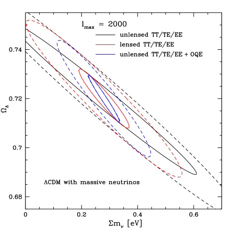
Figures 2 and 3 illustrate the constraints on neutrino mass and dark energy density (cosmological constant) for the different data set types and systematics levels. All figures show 68% confidence level contours; the fiducial model is $\Lambda$CDM, with $\sum m_{\nu}=0.28$ eV. Use of lensing information clearly adds substantial leverage, and measurement of B-modes or the lensing potential play an important role. The two methods of including the full lensing information – adding B-modes or adding the lensing potential – are nearly equivalent (see §VII for further discussion of this).

Figure 2: Cosmological constraints on the neutrino mass and dark energy density in the $\Lambda$CDM fiducial cosmology from CMBpol. Within each panel the contours correspond to systematic cuts at $l_{\rm max}=1000$, 2000, 3000, 4000 from outer to inner. The panels use different data cuts: no lensing (upper left), including lensing from T- and E-modes (upper right), including lensing from T-, E- and B-modes (lower left), and including lensing through the optimal quadratic estimator of the lensing potential (lower right).

Considering the constraints for different systematics levels, we see that much of the lensing leverage is achieved by $l_{\rm max}\approx 2000$. On smaller scales point sources and the SZ effects are expected to dominate over lensing and our limited ability to clean foregrounds through multifrequency observations will likely not allow lensing reconstruction on much smaller scales.

Figure 3: As Fig. 2 but here within each panel the contours correspond to data set types, and the panels use different systematics levels: $l_{\rm max}=1000$ (upper left), 2000 (upper right), 3000 (lower left), 4000 (lower right).

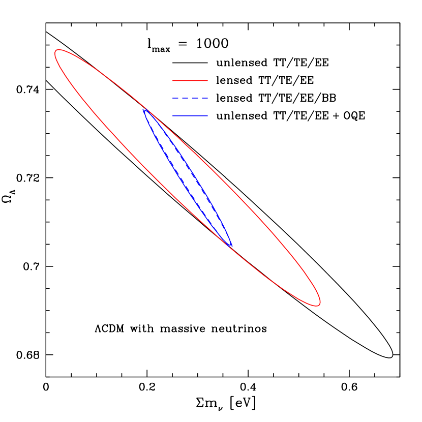
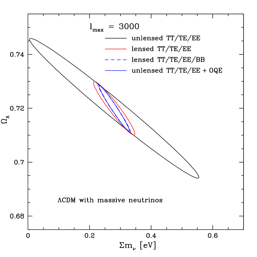
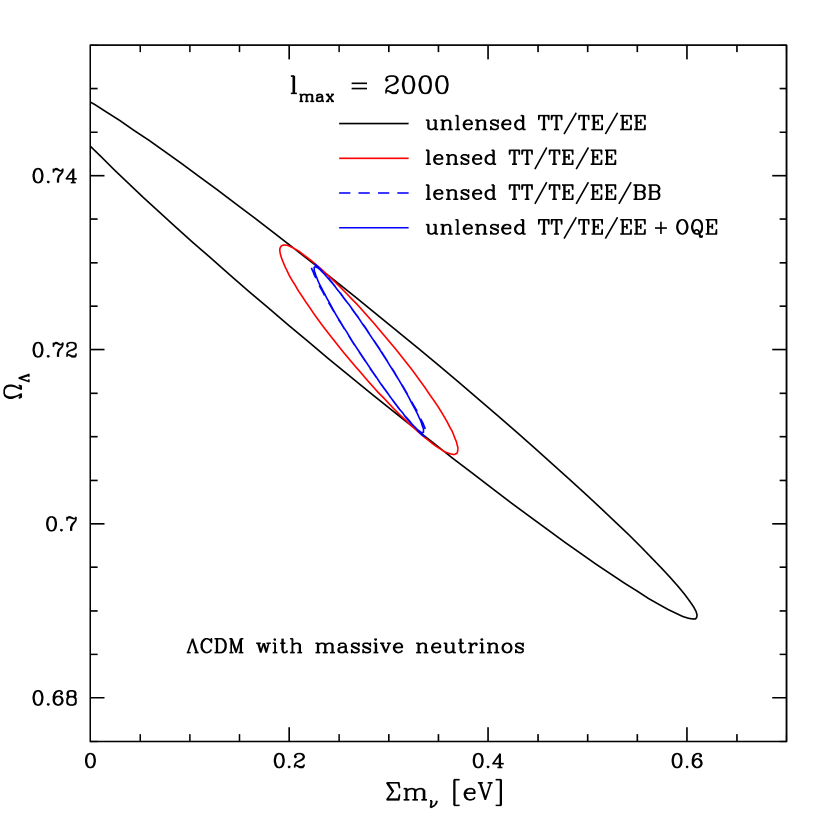
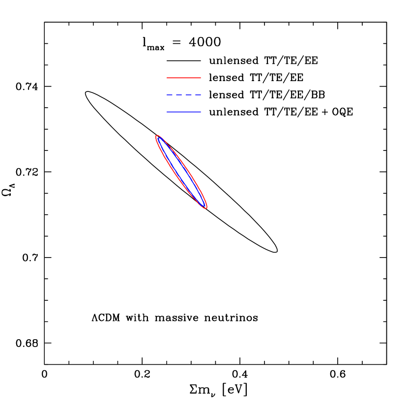
Finally, the dramatic improvement of CMBpol over Planck is clear in Fig. 4. Here we adopt as a standard systematics limit $l_{\rm max}=2000$ and show the confidence contours for each data set type for both experiments. While lensing information does improve the Planck constraints, it runs into a wall due to the relatively high instrumental noise. Furthermore, Planck essentially cannot see B-mode lensing at all (see Fig. 1). This is one of the motivations for intermediate experiments such as PolarBear.

Figure 4: Comparing the cosmological constraints on the neutrino mass and dark energy density in the $\Lambda$CDM fiducial cosmology from Planck (dashed contours) vs. CMBpol (solid), taking $l_{\rm max}=2000$.

IV Adding Dark Energy Dynamics

The cosmic microwave background plays a crucial role in breaking the degeneracies of other probes in order to constrain the properties of dark energy. However, unlensed CMB data itself has very little leverage on learning about dark energy, since the power spectra reflect mostly conditions in the high redshift universe or at best a single weighted average of dark energy influence through the distance to last scattering. With the addition of lensed CMB data we can ask if this improves the leverage on dark energy; we emphasize that it is crucial to consider at least minimally realistic models that include dynamics in the EOS: taking the value of $w$ constant from the present to $z\approx 1100$ is highly non-generic.

It is also important to retain the inclusion of neutrino mass while making this investigation; both neutrino mass and dark energy influence the CMB in many of the same ways, e.g. suppressing structure and causing gravitational potentials to decay. Ignoring neutrino mass could lead to overoptimistic constraints on dark energy. In this section therefore we add $w_{0}$ and $w_{a}$ as fit parameters to the set considered in the previous section. We explore the constraints under the same variety of data cuts as in that section.

The geometric degeneracy due to the acoustic peaks feeling dark energy mostly through the integrated distance to last scattering remains strong, and no reasonable constraints can be placed on the dark energy EOS even with full use of the lensing information. We therefore turn to the issue of complementarity: does the CMB data substantially help other probes of dark energy? In particular we examine complementarity with luminosity distances measured by Type Ia supernovae, since the two probes are well known to strengthen each other fhlt ; huhut . We consider luminosity distances measured to $\sim 1\%$ from $z=0-1.7$, including systematics, as could be provided by a supernova sample realized by a SNAP-type Joint Dark Energy Mission (JDEM)snap .

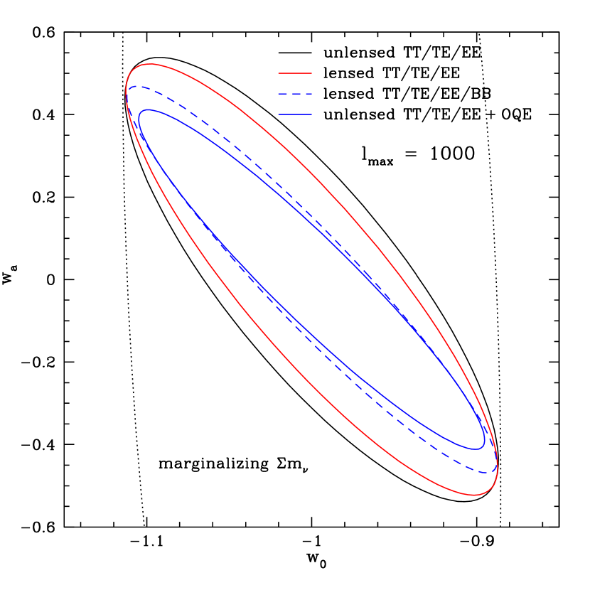
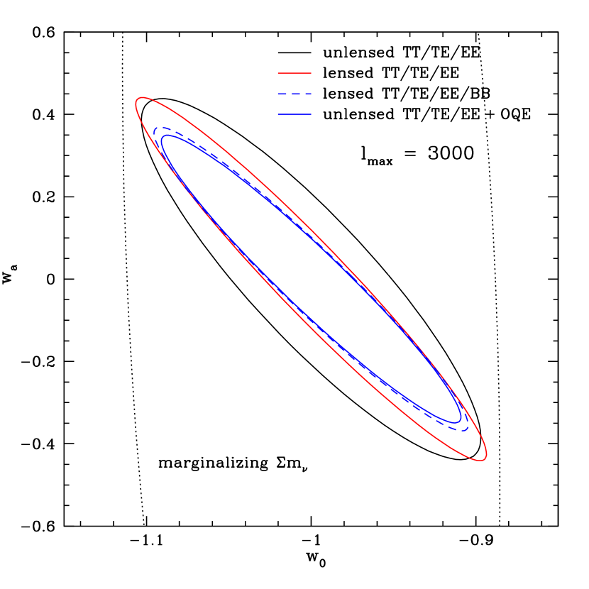
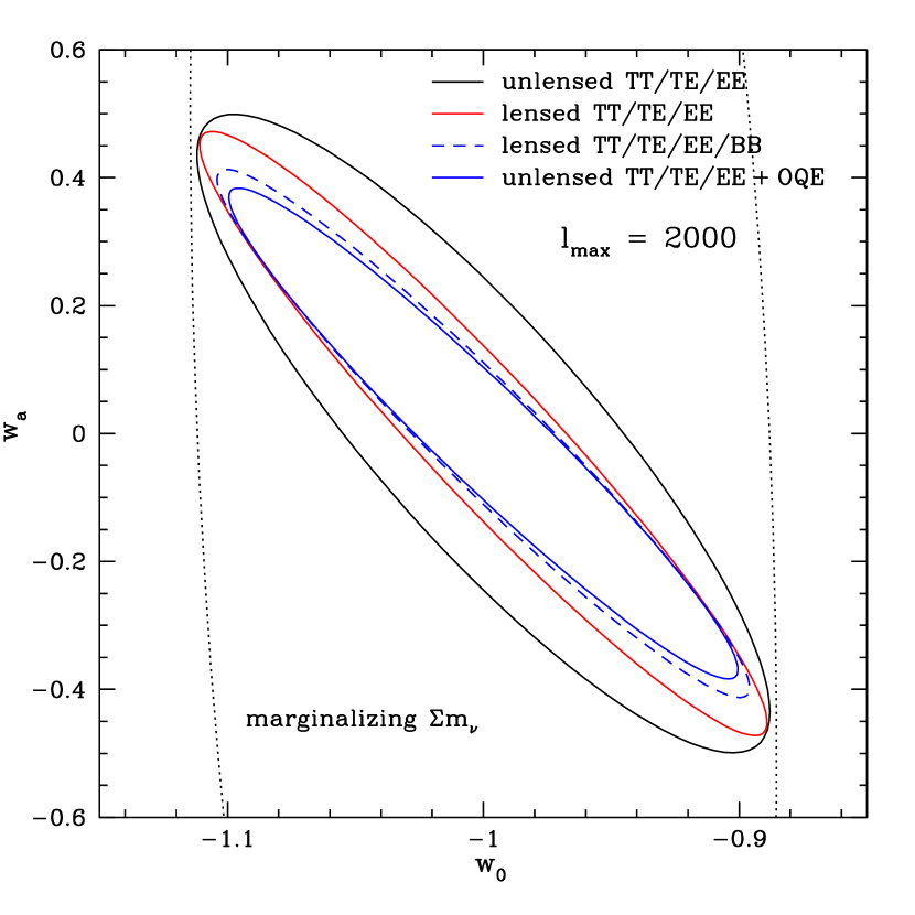
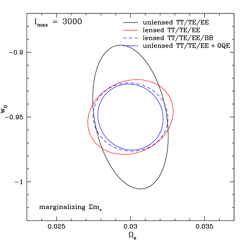
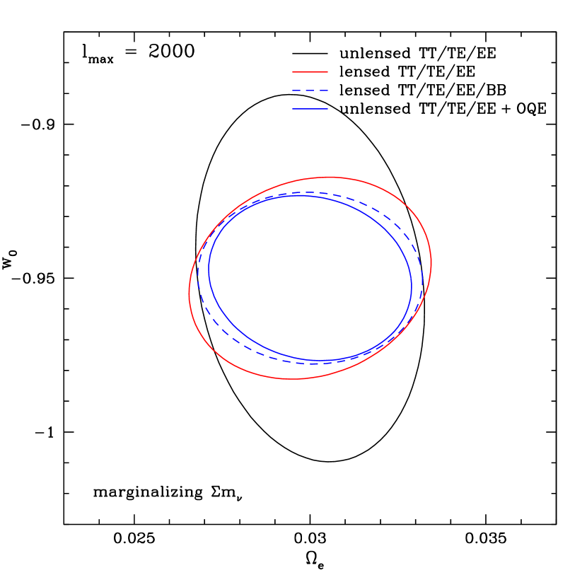
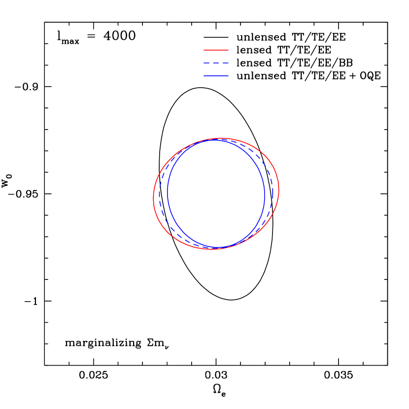
Figure 5 shows the constraints in the $w_{0}$-$w_{a}$ plane, marginalizing over the other seven parameters, for each data set type. The first thing to notice is the clear improvement in measuring the time variation $w_{a}$ over the supernova sample alone due to even unlensed CMB data. Adding lensed CMB data continues to tighten the constraints, in both $w_{0}$ and $w_{a}$, except for the worst systematics level $l_{\rm max}=1000$. Full lensing information continues the improvement modestly on the limits, and somewhat narrows the contours.

Figure 5: Cosmological constraints on the dark energy equation of state parameters $w_{0}$ and $w_{a}$ from CMBpol in combination with SNAP-quality supernova distances. Within each panel the contours correspond to systematic cuts at $l_{\rm max}=1000$, 2000, 3000, 4000 from outer to inner. The panels use different data cuts: no lensing (upper left), including lensing from T- and E-modes (upper right), including lensing from T-, E- and B-modes (lower left), and including lensing through the optimal quadratic estimator of the lensing potential (lower right). The dotted curve gives the constraints from supernovae alone.

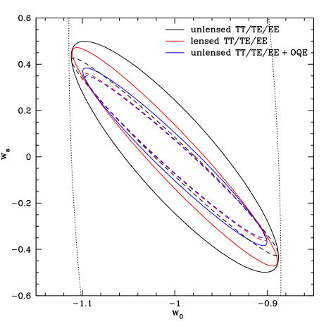
Figure 6 exhibits the analogous situation for different systematic limits $l_{\rm max}$. In contrast to the $\Lambda$CDM case, here the constraints continue to improve for higher $l_{\rm max}$. There are also slight differences between the two methods of fully incorporating lensing: use of B-modes or OQE of the lensing potential. This emphasizes that conclusions on systematics or analysis methods should not be based solely on examination of the vanilla $\Lambda$CDM cosmology. Finally, when systematics are low, $l_{\rm max}=4000$, sufficient information is present in the lensed E-modes that further lensing information is unimportant.

Figure 6: As Fig. 5 but here within each panel the contours correspond to data set types, and the panels use different systematics levels: $l_{\rm max}=1000$ (upper left), 2000 (upper right), 3000 (lower left), 4000 (lower right). Since using lensed TT/EE/TE spectra is not a matter of simply adding to the Fisher matrix from unlensed spectra, it is possible for a lensed contour to lie slightly outside of the unlensed contour, as in the $l_{\rm max}=3000$ case.

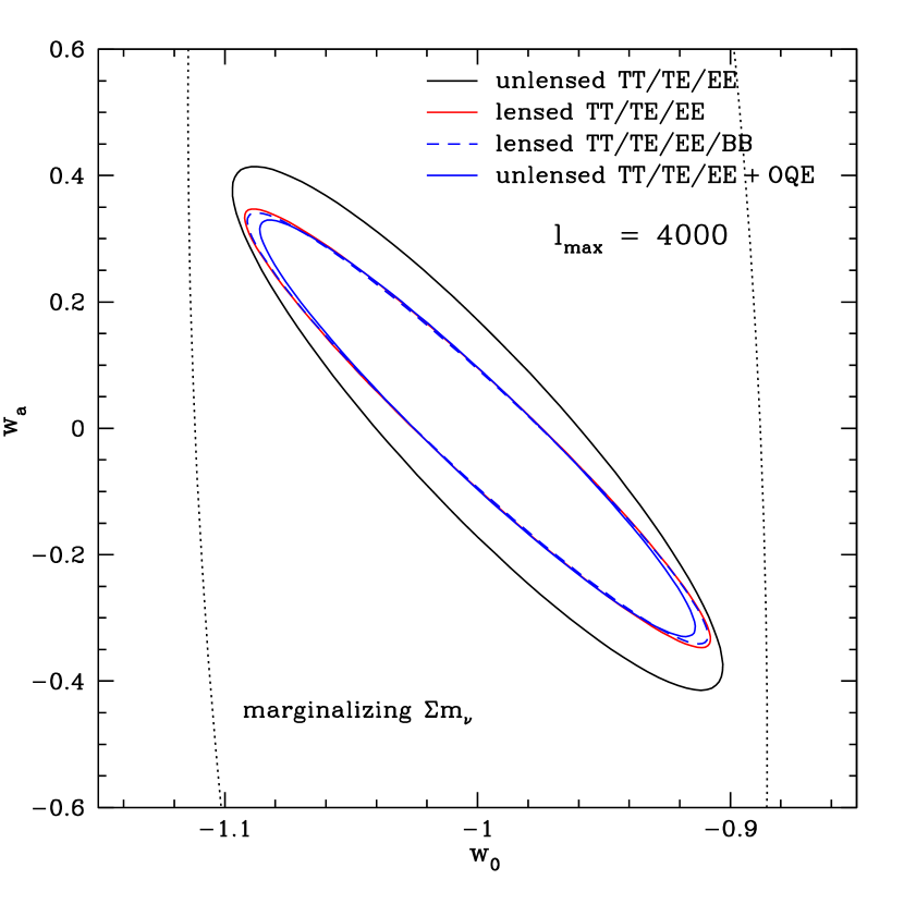
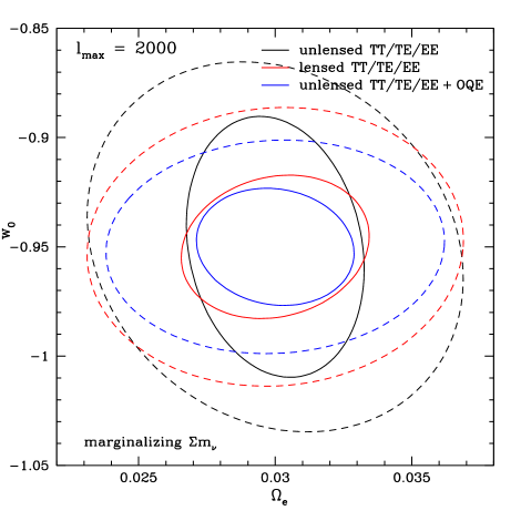
The improvements in dark energy estimation that CMB lensing brings is illustrated in Fig. 7 as a function of experiment. For Planck, again no lensing information beyond E-modes is useful, though the contour area decreases by a factor 1.9 from the unlensed case to the OQE case. By contrast, CMBpol could reduce the likelihood contour area by a factor 4.2 relative to the unlensed Planck case, with the full lensing information helping by a factor 2.7 relative to unlensed CMBpol.

Figure 7: Comparing the cosmological constraints on the dark energy equation of state parameters from Planck (dashed contours) vs. CMBpol (solid), taking $l_{\rm max}=2000$ and including SNAP-quality supernova distances. The dotted curve gives the constraints from supernovae alone.

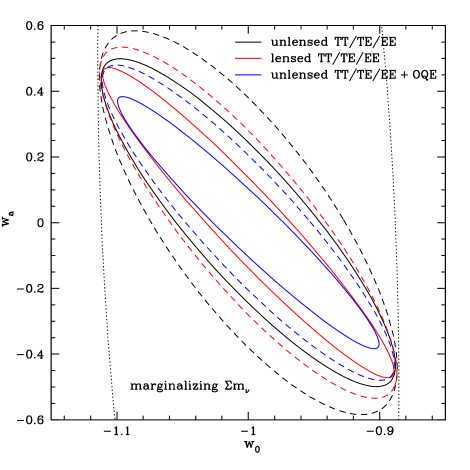
To test the effect of including both neutrino mass and dark energy dynamics, Fig. 8 shows the likelihood contours for the $l_{\rm max}=2000$ CMBpol case, marginalizing over vs. fixing $\sum m_{\nu}$. The fully marginalized uncertainties are $\sigma(\sum m_{\nu})=0.041$, $\sigma(w_{0})=0.066$, $\sigma(w_{a})=0.25$. While the $1\sigma$ limits on the parameters do not change that strongly, the total area of the contour is significantly affected. For the unlensed (fully lensed) case the area increases by a factor 2.9 (1.5) when properly marginalizing over neutrino mass. (This effect would be more severe when considering CMB data alone.) Note that for the CMBpol case the correlation coefficient between $w_{0}$ and $\sum m_{\nu}$ is 0.23 and between $w_{a}$ and $\sum m_{\nu}$ is $-0.41$; while not highly correlated, these are sufficient to give the appreciable effect.

Figure 8: As Fig. 7 for CMBpol only, but here showing the effect of fixing $\sum m_{\nu}$ (dashed contours) rather than marginalizing over it (solid) as is standard for all parameters not shown.

V Exploring Early Dark Energy

In $\Lambda$CDM, the fractional contribution of dark energy density is of order $10^{-9}$ at last scattering. However, many models exist where this can be at the percent level drw , with important impacts on the sound horizon scale and baryon acoustic oscillations, structure formation, and secondary anisotropies drw ; doranrob ; darkages ; sadeh1 ; linrobb ; fllaug08 ; grossi . Such early dark energy models follow from physics where the dark energy traces the energy density of the dominant component of the universe, as in high energy physics and string theory models with dilatation symmetries wett88 .

Although the sound horizon is altered in the presence of early dark energy by $\sim(1-\Omega_{e})^{1/2}$, this shift can be hidden in the temperature power spectrum by compensating changes in the other parameters linrobb . This is problematic for baryon acoustic oscillation experiments, which use the sound horizon as a standard ruler to probe cosmology through distances. More generally, definitive recognition of early dark energy is quite important to have confidence in the accurate estimation of the other parameters, ensuring that they are not biased due to incorrectly assuming no early dark energy. Furthermore, detection of early dark energy would immediately give crucial clues to understanding the nature of dark energy.

Since CMB lensing depends on the growth of structure, it is a good candidate for constraining dark energy. More generally, hints already exist in linrobb that polarization information can help break degeneracies involving early dark energy. Here we carry out a more comprehensive likelihood analysis for unlensed polarization power spectra and examine for the first time CMB lensing constraints on early dark energy. To do this, we employ the parametrization for the fractional dark energy density as a function of scale factor proposed by doranrob ,

$$\Omega_{de}(a)=\frac{\Omega_{de}-\Omega_{e}\left(1-a^{-3w_{0}}\right)}{\Omega_{de}+\Omega_{m}a^{3w_{0}}}+\Omega_{e}\left(1-a^{-3w_{0}}\right),$$ (8)

where $\Omega_{de}$ is the current dark energy density, $\Omega_{e}$ is the constant dark energy density at early times, and $w_{0}$ is the present dark energy equation of state. Hence, the two added parameters $\Omega_{e}$ and $w_{0}$ describe the dark energy properties.

Figure 9 shows the constraints in the $w_{0}$-$\Omega_{e}$ plane, marginalizing over the other seven parameters, for different data set types. The fiducial model has $w_{0}=-0.95$, $\Omega_{e}=0.03$. As in the $w_{0}$-$w_{a}$ case, the CMB degeneracies are too strong to allow constraints by the CMB alone, so we have again folded in supernova distance data (which does not directly constrain $\Omega_{e}$). We see that unlensed power spectra including polarization information can indeed tightly constrain early dark energy. Adding lensed CMB information in fact mostly constrains further $w_{0}$, having minimal effect on $\Omega_{e}$. Recall from §II.1 that out to $z\approx 2$, the early dark energy model looks very much like a standard $w_{0}$-$w_{a}$ model that would not give appreciable early dark energy density. Thus, early dark energy is too early for even the broad redshift kernel of CMB lensing to have significant sensitivity to it.

Figure 9: Cosmological constraints on the early dark energy fraction $\Omega_{e}$ and present equation of state parameter $w_{0}$ from CMBpol in combination with SNAP-quality supernova distances. Within each panel the contours correspond to systematic cuts at $l_{\rm max}=1000$, 2000, 3000, 4000 from outer to inner. The panels use different data cuts: no lensing (upper left), including lensing from T- and E-modes (upper right), including lensing from T-, E- and B-modes (lower left), and including lensing through the optimal quadratic estimator of the lensing potential (lower right).

Figure 10 exhibits the analogous situation for different systematic limits $l_{\rm max}$. Again in contrast to the $\Lambda$CDM case, here the constraints continue to improve for higher $l_{\rm max}$, although less rapidly for $l_{\rm max}\gtrsim 3000$. The fully marginalized uncertainties for the $l_{\rm max}=2000$, full lensing case are $\sigma(\sum m_{\nu})=0.047$, $\sigma(w_{0})=0.018$, $\sigma(\Omega_{e})=0.0019$. This is an impressive constraint on the early dark energy density, able to give definite guidance to the nature of dark energy, ruling out classes of models.

Figure 10: As Fig. 9 but here within each panel the contours correspond to data set types, and the panels use different systematics levels: $l_{\rm max}=1000$ (upper left), 2000 (upper right), 3000 (lower left), 4000 (lower right). Since using lensed TT/EE/TE spectra is not a matter of simply adding to the Fisher matrix from unlensed spectra, it is possible for a lensed contour to lie slightly outside of the unlensed contour.

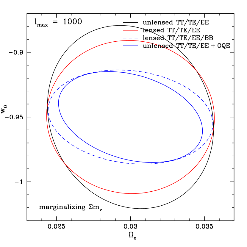
Because CMBpol would have much better polarization measurements than Planck, it will constrain $\Omega_{e}$ better by a factor 2.2, as shown in Fig. 11. The area of the dark energy properties’ confidence contour improves by a factor 3.9.

Figure 11: Comparing the cosmological constraints on the early dark energy fraction $\Omega_{e}$ and present equation of state parameter $w_{0}$ from Planck (dashed contours) vs. CMBpol (solid), taking $l_{\rm max}=2000$ and including SNAP-quality supernova distances.

Finally, we summarize our results for the dark energy and neutrino mass uncertainties in Table 2 for the three cosmological models considered, assuming $l_{\rm max}=2000$. However, one should see the figures for the full contours. Due to degeneracies in the presence of dynamical dark energy, we add supernova data in these cases to constrain the dark energy equation of state, although the uncertainties on $\Omega_{e}$ and $\sum m_{\nu}$ are not strongly affected.

Model	Experiment	$\sigma(w_{0})$	$\sigma(w_{a})$	$\sigma(\Omega_{e})$	$\sigma(\Sigma m_{\nu})$ [eV]
$\Lambda$CDM	Planck	–	–	–	0.11
$\Lambda$CDM	CMBpol	–	–	–	0.036
$w_{0}$-$w_{a}$	Planck+SN	0.073	0.32	–	0.13
$w_{0}$-$w_{a}$	CMBpol+SN	0.066	0.25	–	0.041
$w_{0}$-$\Omega_{e}$	Planck+SN	0.032	–	0.0041	0.15
$w_{0}$-$\Omega_{e}$	CMBpol+SN	0.018	–	0.0019	0.047

Table 2: Uncertainties in parameters beyond standard $\Lambda$CDM for Planck and CMBpol. In all cases, we use unlensed temperature and polarization spectra and the optimal quadratic estimator of the lensing spectrum to extract cosmological information from the CMB data. For cases involving dynamical dark energy we fold in supernova distance information from a SNAP-like JDEM experiment, although this mostly affects only the uncertainties on $w_{0}$, $w_{a}$.

VI Shortcut for Joint Dark Energy Constraints

Figure 12: Joint constraints from CMB and supernovae can be well approximated by simply replacing the CMB data by an appropriately sized prior on the shift parameter $\tilde{d}=\sqrt{\omega_{m}}\,d_{\rm lss}$. [Top panel] Combining Planck data with supernovae, the dark blue (light red) curves represent not using (using) lensing information. These two cases are well approximated by replacing CMB data by $\tilde{d}$ priors of 1.2% and 0.6% respectively. [Bottom panel] Combining CMBpol data with supernovae, the light red curve represents using lensing information. This is fairly well approximated by a $\tilde{d}$ prior of 0.2% (outer black curve). Tighter priors have little effect (see inner black curve). Both panels take $l_{\rm max}=2000$, and the dotted line in both panels is the contour from just supernova data.

As seen in Section IV, when CMB and supernova data are combined, we can obtain strong constraints on the nature of dark energy. While the supernova data dependence on cosmological parameters is straightforward, calculating a CMB Fisher matrix can be quite time consuming. The procedure requires computing multiple CMB spectra using a Boltzmann code (CMBeasy in our case) for different values within a set of cosmological parameters in order to obtain the derivatives of the observables with respect to the cosmological parameters.

To investigate a range of cosmological models it would therefore be quite useful to have a shortcut to calculating the constraints on the dark energy parameters $w_{0},w_{a},\Omega_{DE}$ from CMB data. One such shortcut is historically well known, the shift parameter BE9807103 to encapsulate the information in the temperature power spectrum acoustic peaks. However, as polarization data gets added, other parameters have been suggested as additions, e.g. the acoustic peak scale $l_{A}$ Komatsu:2008hk , although linrpp showed that the shift parameter is still quite accurate. Here we investigate the cosmological constraints from combining CMB temperature, polarization, and possibly deflection, spectra and supernova data, and we show that a simple use of the shift parameter has excellent accuracy.

Specifically, for constraints on the dark energy parameters a strong prior on the shift parameter, or reduced distance to last scattering, $\tilde{d}=\sqrt{\omega_{m}}\,d_{\rm lss}$, is nearly equivalent to the full CMB data, even including polarization and lensing data. That is, the CMB Fisher matrix for $\Omega_{DE},w_{0},w_{a}$ after marginalizing over the other parameters is almost identical to the Fisher matrix calculated from a single constraint on $\tilde{d}\,$. The prior on the quantity $\tilde{d}$ required to match the CMB data depends on the CMB experiment and on whether or not we fix the neutrino mass. We emphasize that the level of the prior does not correspond to the actual determination of $\tilde{d}$ from the experiment, because the prior also encodes the other spectra information. For the CMB experiments we consider, the equivalent prior on $\tilde{d}$ is $0.2\%-1.2\%$.

Note that because early dark energy does not merely affect the projection of the last scattering surface onto our sky, but also affects the shape of the anisotropy spectrum at last scattering directly, we do not expect the $\tilde{d}$ prior to be a complete description there and indeed we found the prior is not effective in this case.

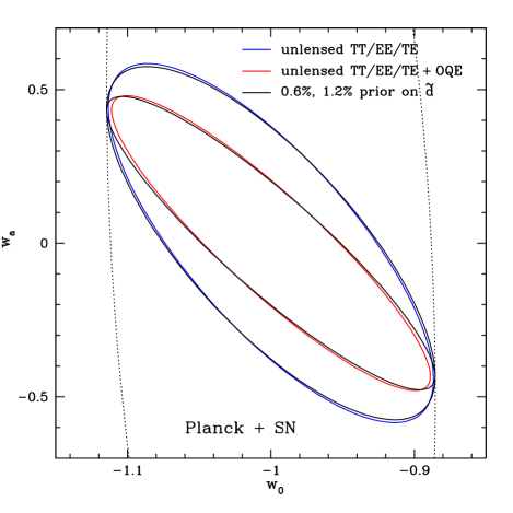
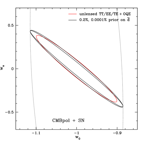
We compare the shift parameter prescription to the use of the actual CMB Fisher matrix in Fig. 12 by considering $1\sigma$ joint contours in the $w_{0}-w_{a}$ plane for CMB + SN. For Planck (top panel), if we marginalize over $\sum m_{\nu}$ and if we do not include the information from CMB lensing, the constraints from the CMB+SN are almost exactly the same as those with a $1.2\%$ prior on $\tilde{d}$. The constraints are improved quite a bit if the lensing information is added. In this case, the constraints are about the same as the constraints one gets with a $0.6\%$ prior on $\tilde{d}$. In the case of fixing $\sum m_{\nu}$ instead of marginalizing over it, the shift parameter prior applies as well, at 0.2% matching the CMB+SN contours whether lensing information is used or not. Interestingly, in the case of fixed $\sum m_{\nu}$, adding lensing information does not appreciably improve the constraints on $w_{0}$ and $w_{a}$ any more.

Note that the Planck experiment can be approximated extremely well by the shift parameter prior in all these cases. The extent $\sigma(w_{0})$, $\sigma(w_{a})$, width $\sigma(w_{p})$, area $1/\sqrt{{\rm det}{\bf F}}$, and orientation of the dark energy EOS contours match, as seen in Fig. 12 and quantified in Table 3.

Data	$\sigma(w_{0})$	$\sigma(w_{a})$	$\sigma(w_{p})$	$\sqrt{{\rm det}{\bf F}}$
SN+Planck	0.073	0.32	0.031	101
SN+0.6% $\tilde{d}$	0.076	0.31	0.032	99
SN+CMBpol	0.066	0.25	0.018	223
SN+0.2% $\tilde{d}$	0.076	0.29	0.017	202

Table 3: Dark energy constraints from supernovae and CMB compared to constraints from supernovae and a prior on the shift parameter $\tilde{d}$. We assume $l_{\rm max}=2000$ and use the optimal quadratic estimator to extract lensing information for both Planck and CMBpol. We marginalize over the sum of the neutrino masses and over the other parameters of the model. Note $\sigma(w_{p})$ is the width of the $w_{0}$-$w_{a}$ contour at $w_{a}=0$ (i.e. the uncertainty in constant $w$) and $\sqrt{{\rm det}{\bf F}}$ is the inverse area of the contour (sometimes used as a figure of merit).

For CMBpol (bottom panel of Fig. 12), the constraints on dark energy can be very well approximated by a $0.2\%$ prior on the shift parameter. This is true independent of whether one fixes $m_{\nu}$ or marginalizes over it because for CMBpol with lensing, fixing $m_{\nu}$ only improves the constraints on $w_{0}$ and $w_{a}$ a little bit compared to marginalizing over $m_{\nu}$ (see Fig. 8). Note that making the prior on $\tilde{d}$ even smaller than $0.2\%$ does not change the contour significantly. To illustrate this, Fig. 12 shows the contour for a prior of $0.0001\%$, essentially fixing $\tilde{d}$. It is almost the same as the contour for $0.2\%$.

The combination of supernova data with a prior on $\tilde{d}$ always gives an ellipse with ends touching the contour from supernovae alone. This means that while both the area enclosed by the contour and the uncertainty in $w_{a}$ may be improved, the uncertainty in $w_{0}$ is the same as the uncertainty from supernova data only. Since Planck constraints are described almost perfectly by the shift parameter, this is also true for Planck. However, once we include precision measurements of polarization by considering CMBpol, the ends of the error ellipse can move away from the “SN only” contour and thus (slightly) improve the constraint on $w_{0}$. This effect cannot be reproduced by the prior on the shift parameter. Hence, for CMBpol, the shift parameter prescription works less well than for Planck, although it is still quite adequate. Again, Table 3 quantifies the accuracy of substituting the prior in place of the full CMB spectra.

VII Progress in Near-term Experiments: PolarBear

In this section we explore the merit of near term ground-based polarization sensitive CMB missions to constrain dark energy and neutrino properties. A number of such experiments are currently being built or have been funded including BICEP/BICEP2 bicep , BRAIN brain , C$\ell$OVER clover , EBEX Oxley:2005dg , QUIET quiet , Spider spider , SPTpol. Here we focus on one of them, PolarBear, as it represents a good combination of the high angular resolution and sensitivity some of these experiments will be capable of.

PolarBear is a ground based telescope with scheduled beginning of operations in 2009, and deployment to Northern Chile in 2010. It plans to observe 2.5% of the sky. The low noise of its detectors will enable this experiment to go beyond Planck in imaging the B-type polarization pattern, which on small scales is a clear signature of gravitational lensing as it cannot be produced by scalar fluctuations. However, the smaller sky coverage does not allow the lensing potential power spectrum to be constrained with as high a signal-to-noise on most scales, making forecasted constraints generally somewhat less good. To describe this experiment’s capabilities, we have adopted specifications from Tran , and the resulting likelihood contours are shown in Fig. 13.

Figure 13: Constraints from the intermediate experiment PolarBear are not as strong as Planck within the restricted inflationary scenario assumed here. Contours are constructed using unlensed TT/TE/EE data plus the optimal quadratic estimator for the lensing spectrum. Blue dotted contours repeat the results for Planck from Figs. 4, 7, 11.

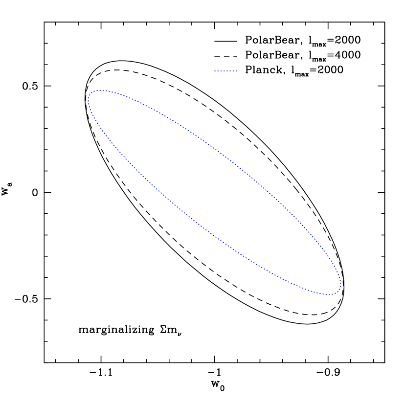
The cosmological constraints from PolarBear lensing reconstruction are less good than those from Planck, despite the significantly lower noise level. The reason is simply that the limited sky coverage does not allow most modes in the temperature, polarization, and lensing potential power spectra to be constrained with as high overall signal-to-noise. However the constraints are still interesting relative to current limits. Moreover, we particularly note that our parameter space has been limited to not include tensor fluctuations, which are a natural consequence of inflationary models. With its low noise level PolarBear will attempt to measure these gravitational waves from inflation and will help break degeneracies between the tensor-to-scalar ratio and other parameters that are present in the Planck data. Furthermore, we have not included running of the scalar spectral index; again, PolarBear’s high resolution and low noise will provide an advantage in breaking degeneracies once running is included.

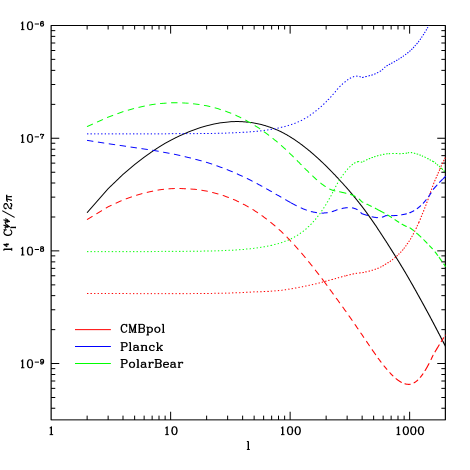
We have found that with Planck the use of the quadratic estimator vs. lensed power spectra leads to a significant improvement of the constraints on parameters to which lensing is sensitive. To be specific, we find a $39\%$ improvement on the neutrino mass scale and a $26\%$ improvement on $\Omega_{\Lambda}$. The improvement in the case of PolarBear and CMBpol is however only marginal. To illuminate this trend, in Figure 14 we plot the power spectra of the lensing potential and lensing reconstruction noises as well as the total errors. The dotted lines show the lensing reconstruction noises for each experiment. PolarBear has better capability to map the lensing potential in the observed patches on the sky than Planck (although it reconstructs far fewer of these patches and therefore the total error is larger than for Planck). The lower lensing noise feeds into the estimation with the optimal quadratic estimator for reconstruction.

Figure 14: The lensing potential power spectrum (solid line) is shown together with the lensing reconstruction noises for the three experiments considered in this work (dotted lines) and the total error on individual multipoles in the lensing potential, a combination of sample variance and noise (dashed lines).

VIII Conclusions

Continued advances are expected in measuring the cosmic microwave background radiation including lower noise and better systematics control, smaller beams and wider surveys, and extension to polarization, cross spectra, and CMB lensing information. These will greatly improve our knowledge of a variety of cosmological parameters related to primordial perturbations. Here we have explored their impact on physics where the CMB has not had as much direct leverage – extensions to the standard model of cosmology such as the necessary neutrino mass and the suspected dynamics of dark energy.

We find the following general points to guide the design and analysis of CMB experiments, both ground based and the CMBpol satellite concept:

• Systematics, such as point sources and other foreground contamination, will affect the lensing potential and other power spectra, and should be removed at the level of at least $l_{\rm max}=2000$. Constraints improve only slowly for higher $l_{\rm max}$ when using the full information in the CMB.

• Analysis of gravitational lensing of the CMB can proceed either through consideration of induced B-mode polarization or through an optimal quadratic estimator directly of the deflection field; the optimum is not steep so the two approaches are nearly equivalent for these purposes with data beyond Planck.

• For exploration of suites of cosmological models, we establish the accuracy of a shortcut in terms of an effective prior on the CMB shift parameter. This is remarkably efficient in summarizing the information from the CMB spectra.

Determination of the sum of neutrino masses can be accomplished by CMBpol with an uncertainty of 0.05 eV, marginalizing over all other parameters including dark energy properties. This corresponds to greater than a $5\sigma$ detection for the fiducial value adopted, and represents a factor 3 improvement over Planck expectations. Restricted to a $\Lambda$CDM cosmology, the constraints tighten by a factor $\sim 1.3$.

Determination of the dynamical properties of dark energy is less powerful. Complementary information, such as from distance measurements, is required with the leverage of the two data sets together allowing significant constraints. The present dark energy equation of state $w_{0}$ could be estimated to 0.07 and the time variation $w_{a}$ to 0.25, including marginalization over other cosmological parameters including neutrino mass. This would improve further as other probes are added. While the marginalized constraints do not improve greatly in going from Planck to CMBpol, the area of the uncertainty contour shrinks by a factor 2.

The most significant impact from the CMB comes within early dark energy models. Here the improvement from Planck to CMBpol is a factor 2 in estimation of both $w_{0}$ (to 0.02 for CMBpol plus distances) and early dark energy density $\Omega_{e}$ (to 0.002 for CMBpol plus distances), while the uncertainty area shrinks by a factor 4. This provides the possibility of a $\sim 10\sigma$ detection of early dark energy, which would immediately revolutionize our physics thinking.

CMB lensing offers an intriguing new window on the universe, especially because of its sensitivity to the properties of expansion and growth in the poorly probed epoch $z\approx 1-4$. Experiments nearly in the process of data collection will teach us not only about the primordial conditions but also about the interesting period when dark energy first becomes significant, as well as establishing a link to terrestrial experiments to measure the neutrino masses.