A glance at singlet states and four-partite correlations

Abstract

Group theoretic methods to construct all $N$-particle singlet states by iterative recursion are presented. These techniques are applied to the quantum correlations of four spin one-half particles in their singlet states. Multipartite quantized systems can be partitioned, and their observables grouped and redefined into condensed correlations.

I Introduction

Improved experimental particle production techniques and potential applications in quantum information theory have stimulated interest in multipartite singlet and other entangled states. In particular, singlet states are among the most useful states in quantum mechanics, as they appear form-invariant under spatial rotations. Hence, a physical property such as uniqueness svozil-2006-uniquenessprinciple or equibalance zeil-99 which holds true in one frame or direction remains to be true in all other frames or directions obtained by spatial rotations.

Yet, the explicit structure of singlet states — although well understood in general terms in group theory — has up to now neither been enumerated nor investigated beyond a few instances for spin one-half and spin one particles. Recent theoretical and experimental studies in multi-particle production (e.g., Ref. egbkzw ) suggest that a more systematic way to generate the complete set of arbitrary $N$-particle singlet states is desirable.

In the present study we first pursue an algorithmic generation strategy, and tabulate some of the first singlet states. The recursive method employed is based on triangle relations and Clebsch-Gordan coefficients (e.g., Ch. 13, Sec. 27 of Ref. messiah-62 ). With this approach, a complete table of all angular momentum states can be enumerated. The singlet states are obtained via the various pathways towards the $j=m=0$ states.

The procedure can best be illustrated by a triangular diagram, where the states in ascending order of angular momentum are drawn against the number of particles. In such a diagram, the “lowest” states correspond to singlet states.

Consider, for the sake of an explicit demonstration of this generation method, a two-dimensional diagram such as the ones depicted in Fig. 1 and in Fig. 2, which represents the “space” or “domain” of all multi-partite states. In such a diagram, the number of particles is represented by the abscissa (the $x$-coordinate) along the positive $x$-axis. The ordinate (the $y$-coordinate) of the state is equal the total angular momentum of the state. Note that a single point may represent many states; all corresponding to an equal number of particles, and all having the same total angular momentum. $N$-partite singlet states can be constructed by starting from the unique state of one particle, then proceeding via all “diagonal” and, whenever possible for integer spins, also “horizontal” pathways (e.g., the “horizontal” path in Fig. 2) consisting of single substeps adding one particle after the other — either diagonally from the lower left to the upper right “$\nearrow$,” or diagonally from the upper left to the lower right “$\searrow$,” or, if possible, also horizontally from left to right “$\rightarrow$” — towards the zero momentum state of $N$ particles. Every diagonal or horizontal substep corresponds to the addition of a single particle. Below we shall explicitly construct singlet states composed from particles of spin one-half and spin one.

In the second part of this article, we present an explicit analysis of the singlet states of four spin one-half particles in terms of their probabilities and expectation functions for spin state measurements. We also investigate the possibility to group the outcomes of the four spin state measurements on each particle to obtain “condensed” observables. Likewise, we consider selection of one or two particles and the resulting correlations. One of our physical motivations for doing so was the question of how such “condensed” observables would perform with respect to violations of classical locality conditions.

II General algorithm for obtaining singlet states

In what follows we present a method to construct all states for a given number of particles. They are the basis to construct non-trivial, e.g., non-“zigzag” singlet states, which are not just products of singlet states of a smaller number of particles. Although only the spin one-half and the spin one cases are explicitly discussed, the method applies to arbitrary spin.

II.1 Spin one-half

We start by considering the spin state of a single spin one-half particle. A second spin one-half particle is added by combining two angular momenta $\frac{1}{2}$ to all possible total angular momenta $l=0$ or $1$. Next, a third particle is introduced by coupling a third angular momentum $\frac{1}{2}$ to all previously derived states. Following the triangle equation, the resulting $j$-values for each $l$ are in the domain

$$|l-j_{3}|\leq j\leq l+j_{3}.$$ (1)

In order to obtain all $N$-particle singlet states, we successively produce all states (not only singlet states) of $N/2$ particles. Note that for $N/2\leq h\leq N$ particles we only need angular momentum states within $0\leq j\leq(N-h)/2$, because the construction method does not allow states with higher angular momentum to “bend diagonally backwards” and finally reach the angular momentum zero singlet state.

Angular momentum states will be written as $|h,j,m,i\rangle$, where $h$ denotes the particle number, $j$ the angular momentum, and $m$ the magnetic quantum number. Note that there may exist many states with equal $h$, $j$ and $m$. Thus $i$ denotes the number of state in an enumeration of all $h$-partite states with identical angular momentum $j$ and magnetic quantum number $m$. In the enumeration scheme chosen, we first take states generated from higher total angular momentum, followed by states with equal total angular momentum for spin one particles, and states with lower total angular momentum. For spin one-half particles, let us define a function $f(j+1,h)$ denoting the total number of states of $h$ particles with total angular momentum $j/2$. This function is tabulated in Table 1 for the spin one-half particle case. The Clebsch-Gordan coefficient is denoted by $\langle j_{1},j_{2},m_{1},m_{2}|j,m\rangle$.

For spin one-half particles, an arbitrary state $|h,j,m,i\rangle$, $h>1$, can be generated from the states with one particle less by adding a particle, thereby increasing or decreasing the total angular momentum of the previous state containing one particle less. Thus, we obtain two different pathways towards $|h,j,m,i\rangle$; one from the total angular momentum $j+{1\over 2}$, symbolized graphically by “$\searrow$,” and one from the total angular momentum $j-{1\over 2}$, symbolized graphically by “$\nearrow$.”

For the sake of demonstration of the method employed, we shall explicitly discuss one of the two cases, in which the addition of one particle $h-1\rightarrow h$ results in a lowering of the total angular momentum by ${1\over 2}$ through $j+{1\over 2}\rightarrow j$, thus representing the diagonal pathway “$\searrow$” from the “upper left” to the “lower right” in a diagram (nonuniquely) representing states as points with coordinates given by the number of particles and the total angular momentum, respectively (e.g., Fig. 1). The first contribution, associated with the magnetic quantum numbers $m-{1\over 2}$ and $+{1\over 2}$, can be constructed from the product state

$$|h-1,j+{1\over 2},m-{1\over 2},i\rangle\otimes|1,{1\over 2},{1\over 2},1\rangle$$ (2)

by multiplying it with the Clebsch-Gordan coefficient

$$\langle j+{1\over 2},m-{1\over 2},{1\over 2},{1\over 2}|j,m\rangle.$$ (3)

Similarly, the second contribution to $|h,j,m,i\rangle$, associated with the magnetic quantum numbers $m+{1\over 2}$ and $-{1\over 2}$, can be constructed via the product state

$$|h-1,j+{1\over 2},m+{1\over 2},i\rangle\otimes|1,{1\over 2},-{1\over 2},1\rangle,$$ (4)

multiplied with the Clebsch-Gordan coefficient

$$\langle j+{1\over 2},m+{1\over 2},{1\over 2},-{1\over 2}|j,m\rangle.$$ (5)

Adding the two results, we obtain the state $|h,j,m,i\rangle$; i.e.,

$$\begin{array}[]{rcl}|h,j,m,i\rangle&=&\langle j+{1\over 2},m-{1\over 2},{1\over 2},{1\over 2}|j,m\rangle|h-1,j+{1\over 2},m-{1\over 2},i\rangle\otimes|1,{1\over 2},{1\over 2},1\rangle+\\ &&\;+\langle j+{1\over 2},m+{1\over 2},{1\over 2},-{1\over 2}|j,m\rangle|h-1,j+{1\over 2},m+{1\over 2},i\rangle\otimes|1,{1\over 2},-{1\over 2},1\rangle.\end{array}$$ (6)

We do this for $m=-j,\ldots,j$ and for all states labeled by the state number $i=1,2,\ldots$, $f((2j+1)+1,h-1)$. Recall that $f(j+1,h)$ denotes the total number of states of $h$ particles with angular momentum $j/2$. It can be computed by counting the number of all states generated by all possible pathways in the construction method described above.

Similarly, if $j$ is greater than zero, we obtain the state $|h,j,m,i\rangle$ from the diagonal pathway “$\nearrow$,” starting from the states $|h-1,j-{1\over 2},m-{1\over 2},i\rangle$ and $|h-1,j-{1\over 2},m+{1\over 2},i\rangle$ of $h-1$ particles and total angular momentum $j-{1\over 2}$ by adding a single particle via

$$\langle j-{1\over 2},m-{1\over 2},{1\over 2},{1\over 2}|j,m\rangle|h-1,j-{1\over 2},m-{1\over 2},i\rangle\otimes|1,{1\over 2},{1\over 2},1\rangle$$ (7)

and

$$\langle j-{1\over 2},m+{1\over 2},{1\over 2},-{1\over 2}|j,m\rangle|h-1,j-{1\over 2},m+{1\over 2},i\rangle\otimes|1,{1\over 2},-{1\over 2},1\rangle.$$ (8)

This procedure is carried out for $m=-j,\ldots,j$ and $i$ satisfying

$$f((2j+1)+1,h-1)+1\leq i\leq f((2j+1)+1,h-1)+f((2j+1)-1,h-1).$$ (9)

A concrete example is drawn in Fig. 1.

1pt		1pt
a)		b)

Figure 1: Construction of both singlet states a) and b) of four spin one-half particles. Concentric circles indicate the target states. The second state is a “zigzag” state composed by the product of two two-partite singlet states.

It contains the pathways leading to the construction of both singlet states of four spin one-half particles.

For spin one-half particles, the function $f(j+1,h)$ denoting the total number of states of $h$ particles with total angular momentum $j/2$ is tabulated in Table 1. The bottom line above the axis contains the number of different orthogonal singlet states.

$j$
5										1
$\frac{9}{2}$									1		10
4								1		9		54
$\frac{7}{2}$							1		8		44		208
3						1		7		35		154		637
$\frac{5}{2}$					1		6		27		110		429		1638
2				1		5		20		75		275		1001		3640
$\frac{3}{2}$			1		4		14		48		165		572		2002		7072
1		1		3		9		28		90		297		1001		3432		11934
$\frac{1}{2}$	1		2		5		14		42		132		429		1430		4862		16796
0		1		2		5		14		42		132		429		1430		4862		16796
	1	2	3	4	5	6	7	8	9	10	11	12	13	14	15	16	17	18	19	20	$N$

Table 1: Enumeration of the total numbers of states contributing to a calculation of singlet states up to 20 spin one-half particles. The bottom line above the axis shows the actual number of different orthogonal singlet states.

The singlet states of up to six spin one-half particles are explicitly enumerated in Table 2.

N	#
2	1	$\frac{1}{{\sqrt{2}}}\big{(}|+-\rangle-|-+\rangle\big{)};$
4	1	$-\frac{1}{2\sqrt{3}}\big{(}|-+-+\rangle+|-++-\rangle+|+--+\rangle+|+-+-\rangle\big{)}+$
		$+\frac{1}{\sqrt{3}}\big{(}|--++\rangle+|++--\rangle\big{)};$
4	2	$\big{(}-\frac{1}{{\sqrt{2}}}|-+\rangle+\frac{1}{{\sqrt{2}}}|+-\rangle\big{)}^{2};$
6	1	$-\frac{1}{2}|---+++\rangle+-\frac{1}{6}\big{(}|-++--+\rangle+|-++-+-\rangle+$
		$+|-+++--\rangle+|+-+--+\rangle+|+-+-+-\rangle+$
		$+|+-++--\rangle+|++---+\rangle+|++--+-\rangle+$
		$+|++-+--\rangle\big{)}+\frac{1}{6}\big{(}|--+-++\rangle+|--++-+\rangle+$
		$+|--+++-\rangle+|-+--++\rangle+|-+-+-+\rangle+$
		$+|-+-++-\rangle+|+---++\rangle+|+--+-+\rangle+$
		$+|+--++-\rangle\big{)}+\frac{1}{2}|+++---\rangle;$
6	2	$-\frac{{\sqrt{2}}}{3}|--+-++\rangle+-\frac{1}{3{\sqrt{2}}}\big{(}|-+++--\rangle+|+-++--\rangle+$
		$+|++---+\rangle+|++--+-\rangle\big{)}+-\frac{1}{6{\sqrt{2}}}\big{(}|-+-+-+\rangle+$
		$+|-+-++-\rangle+|+--+-+\rangle+|+--++-\rangle\big{)}+$
		$+\frac{1}{6{\sqrt{2}}}\big{(}|-++--+\rangle+|-++-+-\rangle+|+-+--+\rangle+$
		$+|+-+-+-\rangle\big{)}+\frac{1}{3{\sqrt{2}}}\big{(}|--++-+\rangle+|--+++-\rangle+$
		$+|-+--++\rangle+|+---++\rangle\big{)}+\frac{{\sqrt{2}}}{3}|++-+--\rangle;$
6	3	$-\frac{1}{{\sqrt{6}}}\big{(}|-+--++\rangle+|-+++--\rangle\big{)}+-\frac{1}{2{\sqrt{6}}}\big{(}|+--+-+\rangle+$
		$+|+--++-\rangle+|+-+--+\rangle+|+-+-+-\rangle\big{)}+$
		$+\frac{1}{2{\sqrt{6}}}\big{(}|-+-+-+\rangle+|-+-++-\rangle+|-++--+\rangle+$
		$+|-++-+-\rangle\big{)}+\frac{1}{{\sqrt{6}}}\big{(}|+---++\rangle+|+-++--\rangle\big{)};$
6	4	$-\frac{1}{{\sqrt{6}}}\big{(}|--++-+\rangle+|++---+\rangle\big{)}+-\frac{1}{2{\sqrt{6}}}\big{(}|-+-++-\rangle+$
		$+|-++-+-\rangle+|+--++-\rangle+|+-+-+-\rangle\big{)}+$
		$+\frac{1}{2{\sqrt{6}}}\big{(}|-+-+-+\rangle+|-++--+\rangle+|+--+-+\rangle+$
		$+|+-+--+\rangle\big{)}+\frac{1}{{\sqrt{6}}}\big{(}|--+++-\rangle+|++--+-\rangle\big{)};$
6	5	$\big{(}-\frac{1}{{\sqrt{2}}}|-+\rangle+\frac{1}{{\sqrt{2}}}|+-\rangle\big{)}^{3}.$

Table 2: First singlet states of $N$ spin one-half particles.

II.2 Spin one

The construction of the singlet states of spin one particles follows similar rules as in the case of spin one-half particles. One example is the construction of the singlet state consisting of three spin one particles drawn in Fig. 2. Note that in this case, as for all particles of integer spin, there are three possible subpaths per addition of one particle; two diagonal “$\nearrow$” and “$\searrow$” pathways as in the case for spin one-half particles, as well as one horizontal “$\rightarrow$.”

1pt

Figure 2: Construction of the singlet state of three spin one particles. Note that for integer spin, there are three possible subpaths per addition of one particle; two diagonal “$\nearrow$” and “$\searrow$,” as well as one horizontal “$\rightarrow$.”

Table 3 enumerates the numbers of states contributing to a calculation of singlet states up to 18 spin one particles. The bottom line above the axis shows the actual number of different orthogonal singlet states. The singlet states of up to four spin one (with one singlet state of 5) particles are explicitly enumerated in Table 4.

$j$
9									1
8								1	8	45
7							1	7	36	155	605
6						1	6	28	111	405	1397	4642
5					1	5	21	76	258	837	2640	8162	24882
4				1	4	15	49	154	468	1398	4125	12078	35178	102102
3			1	3	10	29	84	238	672	1890	5313	14938	42042	118482	334425
2		1	2	6	15	40	105	280	750	2025	5500	15026	41262	113841	315420	877320
1	1	1	3	6	15	36	91	232	603	1585	4213	11298	30537	83097	227475	625992	1730787
0		1	1	3	6	15	36	91	232	603	1585	4213	11298	30537	83097	227475	625992	1730787
	1	2	3	4	5	6	7	8	9	10	11	12	13	14	15	16	17	18	$N$

Table 3: Enumeration of the total numbers of states contributing to a calculation of singlet states up to 18 spin one particles. The bottom line above the axis shows the actual number of different orthogonal singlet states.

N	#
2	1	$\frac{1}{{\sqrt{3}}}\big{(}-|0,0\rangle+|-1,1\rangle+|1,-1\rangle\big{)};$
3	1	$-\frac{1}{{\sqrt{6}}}\big{(}|-1,0,1\rangle+|0,1,-1\rangle+|1,-1,0\rangle\big{)}+$
		$+\frac{1}{{\sqrt{6}}}\big{(}|-1,1,0\rangle+|0,-1,1\rangle+|1,0,-1\rangle\big{)};$
4	1	$-\frac{1}{2{\sqrt{5}}}\big{(}|-1,0,0,1\rangle+|-1,0,1,0\rangle+|0,-1,0,1\rangle+|0,-1,1,0\rangle+$
		$+|0,1,-1,0\rangle+|0,1,0,-1\rangle+|1,0,-1,0\rangle+|1,0,0,-1\rangle\big{)}+$
		$+\frac{1}{6{\sqrt{5}}}\big{(}|-1,1,-1,1\rangle+|-1,1,1,-1\rangle+|1,-1,-1,1\rangle+|1,-1,1,-1\rangle\big{)}+$
		$+\frac{1}{3{\sqrt{5}}}\big{(}|-1,1,0,0\rangle+|0,0,-1,1\rangle+|0,0,1,-1\rangle+|1,-1,0,0\rangle\big{)}+$
		$+\frac{2}{3{\sqrt{5}}}|0,0,0,0\rangle+\frac{1}{{\sqrt{5}}}\big{(}|-1,-1,1,1\rangle+|1,1,-1,-1\rangle\big{)};$
4	2	$-\frac{1}{2{\sqrt{3}}}\big{(}|-1,0,1,0\rangle+|-1,1,-1,1\rangle+|0,-1,0,1\rangle+|0,1,0,-1\rangle+$
		$+|1,-1,1,-1\rangle+|1,0,-1,0\rangle\big{)}+\frac{1}{2{\sqrt{3}}}\big{(}|-1,0,0,1\rangle+|-1,1,1,-1\rangle+$
		$+|0,-1,1,0\rangle+|0,1,-1,0\rangle+|1,-1,-1,1\rangle+|1,0,0,-1\rangle\big{)};$
4	3	$\big{(}\frac{1}{{\sqrt{3}}}\big{(}-|0,0\rangle+|-1,1\rangle+|1,-1\rangle\big{)}\big{)}^{2};$
5	1	$-{\sqrt{\frac{2}{15}}}|-1,-1,0,1,1\rangle+-\frac{1}{{\sqrt{30}}}\big{(}|-1,0,1,0,0\rangle+|0,-1,1,0,0\rangle+$
		$+|0,0,-1,0,1\rangle+|0,0,-1,1,0\rangle+|0,1,1,-1,-1\rangle+$
		$+|1,0,1,-1,-1\rangle+|1,1,-1,-1,0\rangle+|1,1,-1,0,-1\rangle\big{)}+$
		$+-\frac{1}{2{\sqrt{30}}}\big{(}|-1,0,1,-1,1\rangle+|-1,0,1,1,-1\rangle+|-1,1,-1,0,1\rangle+$
		$+|-1,1,-1,1,0\rangle+|0,-1,1,-1,1\rangle+|0,-1,1,1,-1\rangle+$
		$+|0,1,0,-1,0\rangle+|0,1,0,0,-1\rangle+|1,-1,-1,0,1\rangle+$
		$+|1,-1,-1,1,0\rangle+|1,0,0,-1,0\rangle+|1,0,0,0,-1\rangle\big{)}+$
		$+\frac{1}{2{\sqrt{30}}}\big{(}|-1,0,0,0,1\rangle+|-1,0,0,1,0\rangle+|-1,1,1,-1,0\rangle+$
		$+|-1,1,1,0,-1\rangle+|0,-1,0,0,1\rangle+|0,-1,0,1,0\rangle+$
		$+|0,1,-1,-1,1\rangle+|0,1,-1,1,-1\rangle+|1,-1,1,-1,0\rangle+$
		$+|1,-1,1,0,-1\rangle+|1,0,-1,-1,1\rangle+|1,0,-1,1,-1\rangle\big{)}+$
		$+\frac{1}{{\sqrt{30}}}\big{(}|-1,-1,1,0,1\rangle+|-1,-1,1,1,0\rangle+|-1,0,-1,1,1\rangle+$
		$+|0,-1,-1,1,1\rangle+|0,0,1,-1,0\rangle+|0,0,1,0,-1\rangle+$
		$+|0,1,-1,0,0\rangle+|1,0,-1,0,0\rangle\big{)}+{\sqrt{\frac{2}{15}}}|1,1,0,-1,-1\rangle;$

Table 4: First singlet states of $N$ spin one particles.

There always exist trivial “zigzag” singlet states which are the product of $r$ two-particle singlet states stemming from the rising and lowering of consecutive states. The situation is depicted in Fig. 3. For $j=1$ and $N=3r$ there exist “zigzag” singlet states, which are the product of $r$ three-particle singlet states. For singlet states with $N=2r+3t$ ($r,t$ integer) there exist singlet states being the product of $r$ two-particle singlet states and $t$ three-particle singlet states.

1pt

Figure 3: Construction of the “zigzag” singlet state of $N$ particles which effectively is a product state of $\frac{N}{2}$ spin $l$ particle states.

III Symmetries

In what follows we shall discuss the symmetry behavior of singlet states. In our approach the singlet states are orthogonal to each other. This can be demonstrated by considering the formula Hagedorn

$$\begin{array}[]{rcl}\langle(j_{1}^{\prime}j_{2}^{\prime})jm|(j_{1}j_{2})jm\rangle&=&\sum_{m_{1}^{\prime}+m_{2}^{\prime}=m,m_{1}+m_{2}=m}\langle(j_{1}^{\prime}j_{2}^{\prime})jm|j_{1}^{\prime}m_{1}^{\prime}j_{2}^{\prime}m_{2}^{\prime}\rangle\times\\ &&\langle j_{1}^{\prime}m_{1}^{\prime}j_{2}^{\prime}m_{2}^{\prime}|j_{1}m_{1}j_{2}m_{2}\rangle\langle j_{1}m_{1}j_{2}m_{2}|(j_{1}j_{2})jm\rangle\\ &=&\delta_{j_{1}j_{1}^{\prime}}\delta_{j_{2}j_{2}^{\prime}}\delta_{m_{1}m_{1}^{\prime}}\delta_{m_{2}m_{2}^{\prime}},\end{array}$$ (10)

where $|(j_{1}j_{2})jm\rangle$ stands for a state of total angular momentum $j$ and magnetic quantum number $m$, composed of two parts having angular momentum $j_{1}$ and $j_{2}$, respectively. States stemming from different $j_{1}$ values are orthogonal to each other. Hence, also the singlet states derived from them are orthogonal. By iteration it follows that even singlet states stemming from the same $j_{1}$ are orthogonal. The method allows us to construct the full basis for each singlet space which has the appropriate dimension.

III.1 Sign changes of magnetic quantum numbers

For the Clebsch-Gordan coefficients the following formula holds

$$\langle j_{1},-m_{1},j_{2},-m_{2}|j,-m\rangle=(-1)^{j_{1}+j_{2}-j}\langle j_{1}m_{1}j_{2}m_{2}|jm\rangle.$$ (11)

III.1.1 Spin one-half

In what follows, the symmetries of singlet spin one-half particle states are investigated. For a coupling $j$ to $j+\frac{1}{2}$, the Clebsch-Gordan coefficients satisfy

$$\begin{array}[]{rcl}\langle j,-m-\frac{1}{2},\frac{1}{2},\frac{1}{2}|j+\frac{1}{2},-m\rangle&=&(-1)^{0}\langle j,m+\frac{1}{2},\frac{1}{2},-\frac{1}{2}|j+\frac{1}{2},m\rangle\\ \langle j,m+\frac{1}{2},\frac{1}{2},-\frac{1}{2}|j+\frac{1}{2},m\rangle&=&(-1)^{0}\langle j,-m-\frac{1}{2},\frac{1}{2},\frac{1}{2}|j+\frac{1}{2},-m\rangle.\end{array}$$

If all the magnetic quantum numbers reverse their signs, the Clebsch-Gordan coefficients stay the same. Coupling $j+\frac{1}{2}$ to $j$ results in

$$\begin{array}[]{rcl}\langle j+\frac{1}{2},m,\frac{1}{2},\frac{1}{2}|j,m+\frac{1}{2}\rangle&=&(-1)^{1}\langle j+\frac{1}{2},-m,\frac{1}{2},-\frac{1}{2}|j,-m-\frac{1}{2}\rangle\\ \langle j+\frac{1}{2},-m,\frac{1}{2},-\frac{1}{2}|j,-m-\frac{1}{2}\rangle&=&(-1)^{1}\langle j+\frac{1}{2},m,\frac{1}{2},\frac{1}{2}|j,m+\frac{1}{2}\rangle.\end{array}$$

In this case, all the Clebsch-Gordan coefficients change their signs.

We conclude that the symmetry behavior remains the same if one passes from the angular momentum subspace $|N,J\rangle$ to the angular momentum subspace $|N+1,J+{1\over 2}\rangle$. By passing from the subspace $|N,J\rangle$ to the subspace $|N+1,J-{1\over 2}\rangle$ the symmetry behaviour changes from even to odd and from odd to even, respectively. A graphical representation of this property is depicted in Fig. 4. In particular, the singlet states where $N$ is $k\cdot 2\cdot 2$ (k is an integer) are even, and the ones where $N$ is $2\cdot(2k+1)$ are odd.

1pt

Figure 4: Symmetry behavior of spin one-half particles. Even and odd subspaces are denoted by concentric and filled circles, respectively. The numbers denote the dimensions of the subspaces. The first number stands for the number of states $|h,j\rangle$, and the second number stands for the $2j+1$ projections. Arrows represent the direction of the coupling.

III.1.2 Spin one

Let us now consider the $j=1$ case first. For the coupling of $j$ to $j+1$, the symmetry described above implies

$$\begin{array}[]{rcl}\langle j,-m-1,1,1|j+1,-m\rangle&=&(-1)^{0}\langle j,m+1,1,-1|j+1,m\rangle,\\ \langle j,-m,1,0|j+1,-m\rangle&=&(-1)^{0}\langle j,m,1,0|j+1,m\rangle;\end{array}$$ (12)

i.e., the Clebsch-Gordan coefficients are the same. For the coupling of $j$ to $j$,

$$\begin{array}[]{rcl}\langle j,-m-1,1,1|j,-m\rangle&=&(-1)^{1}\langle j,m+1,1,-1|j,m\rangle,\\ \langle j,-m,1,0|j,-m\rangle&=&(-1)^{1}\langle j,m,1,0|j,m\rangle;\end{array}$$ (13)

i.e., all Clebsch-Gordan coefficients change sign. Similarly for the coupling of $j+1$ to $j$,

$$\begin{array}[]{rcl}\langle j+1,m,1,1|j,m+1\rangle&=&(-1)^{2}\langle j+1,-m,1,-1|j,-m-1\rangle,\\ \langle j+1,m,1,0|j,m\rangle&=&(-1)^{2}\langle j+1,-m,1,0|j,-m\rangle;\end{array}$$ (14)

i.e., they all stay the same.

Using these symmetries, we conclude that the symmetry behaviour remains the same if one passes from the angular momentum subspace $|N,j\rangle$ to the angular momentum subspace $|N+1,j+1\rangle$. The symmetry behaviour does not change for coupling $|N,j+1\rangle$ to $|N+1,j\rangle$. Coupling $|N,j\rangle$ to $|N+1,j\rangle$ changes the symmetry behaviour from even to odd and from odd to even. The situation is depicted in Fig. 5. $N$-particle singlet states with $N$ even are even, whereas $N$-particle singlet states with $N$ odd are odd.

1pt

Figure 5: Symmetries of spin one particle states. Even subspaces are denoted by concentric circles, odd subspaces are denoted by filled circles. The numbers denote the dimensions of the subspaces. The first number stands for the number of states $|h,j\rangle$ and the second stands for the $2j+1$ projections. Arrows represent the way of coupling.

III.2 Symmetric group

Let us consider the permutations of the $N$ magnetic quantum numbers in every product state of $N$ particles. More explicitly, since every permutation of $N$ particles can be written as the product of $N-1$ transpositions, we shall study the effects of $N-1$ transpositions. We analyze $N-1$ transpositions of the form $(j,j+1)$, the transposition of $j$ and $j+1$ which generate the whole symmetric group, and in particular all the $N\cdot(N-1)/2$ transpositions, since $(j,k+1)=(k,k+1)(j,k)(k,k+1)$. Therefore, we consider the class $(2\;1^{N-2})$ of all two particle transpositions. Each irreducible representation can be labeled by an ordered partition of integers which corresponds to a specific Young diagram.

As stated in App. D, Sec. 14 of Ref. messiah-62 , the space spanned by the vectors of total spins $(SM)$ formed by $N$ identical spins ${1\over 2}$ is associated with an irreducible representation of $S_{N}$, the representation whose Young diagram corresponds to the partition $[{1\over 2}N+S,{1\over 2}N-S]$ of the integer $N$. It is apparent that the Young diagrams for the irreducible components of the representation of $S_{N}$ have at most two lines. For $N>2$, any state contains at least two individual spins in the same state. Suppose the state contains the factor $u_{+}^{(i)}u_{+}^{(j)}$; i.e., $m_{i},m_{j}={1\over 2}$. Since $A={1\over 2}(1-(i,j))$ is the antisymmetrizer and ${1\over 2}(1-(i,j))u_{+}^{(i)}u_{+}^{(j)}=0$, it follows that $A|jm\rangle=0$.

Using the theorem mentioned above, the Young diagrams of the irreducible spaces of the $N$-particle singlet states correspond to the partitions $[{1\over 2}N,{1\over 2}N]$. Hence the two-particle singlet state (sometimes referred to as the “Bell” state) is an antisymmetric one-dimensional space. The four- and six-particle singlet spaces form a two- and a five-dimensional irreducible space whose Young diagrams are of the form $[2,2]$ and $[3,3]$. Using the formula for the dimension of an irreducible representation having the partition $[\lambda]$ (e.g., Ref. wybourne )

$$f^{\lambda}=n!\,\frac{\Pi_{i<j\leq k}(\lambda_{i}-\lambda_{j}+j-i)}{\Pi^{k}_{i=1}(\lambda_{i}+k-i)!},$$ (15)

the dimension can be verified.

IV Four spin one-half particle correlations

Singlet states $|\Psi_{d,n,i}\rangle$ can be labeled by three numbers $d$, $n$ and $i$, denoting the number $d$ of outcomes associated with the dimension of Hilbert space per particle, the number $n$ of participating particles, and the state count $i$ in an enumeration of all possible singlet states of $n$ particles of spin $j=(d-1)/2$, respectively. To begin with the analysis of four-partite correlations, consider four spin one-half particles in one of the two singlet states enumerated in Table 2 and computed by following the “paths” indicated in Fig. 1; i.e.,

$$|\Psi_{2,4,1}\rangle = {1\over\sqrt{3}}\Bigl{[}|++--\rangle+|--++\rangle$$ (16)

$$\qquad\qquad-{1\over 2}\bigl{(}|+-\rangle+|-+\rangle\bigr{)}\bigl{(}|+-\rangle+|-+\rangle\bigr{)}\Bigr{]},$$

$$|\Psi_{2,4,2}\rangle = \left(|\Psi_{2,2,1}\rangle\right)^{2}={1\over 2}\bigl{(}|+-\rangle-|-+\rangle\bigr{)}\bigl{(}|+-\rangle-|-+\rangle\bigr{)},$$ (17)

where $|\Psi_{2,2,1}\rangle=\frac{1}{\sqrt{2}}\bigl{(}|+-\rangle-|-+\rangle\bigr{)}$ is the two particle singlet “Bell” state.

These pure states have an explicit vector space representation as orthogonal vectors. The two states corresponding to spin “up” and “down” correspond to $|+\rangle\equiv{\hat{\bf e}}_{1}=(1,0)$ and $|-\rangle\equiv{\hat{\bf e}}_{2}=(0,1)$. Product states can be represented by the tensor or Kronecker product, which, for two arbitrary vectors ${\bf a}=(a_{1},a_{2},\ldots,a_{n})$ and ${\bf b}=(b_{1},b_{2},\ldots,b_{m})$, can be represented by

$${\bf a}\otimes{\bf b}=(a_{1}{\bf b},a_{2}{\bf b},\ldots,a_{n}{\bf b})=(a_{1}b_{1},a_{1}b_{2},\ldots,a_{n}b_{m}).$$ (18)

Thus, by summing up all product sates, the two singlet states have a vector representation as

$$\hat{\Psi}_{2,4,1} = {1\over\sqrt{3}}\Bigl{[}{\hat{\bf e}}_{1}\otimes{\hat{\bf e}}_{1}\otimes{\hat{\bf e}}_{2}\otimes{\hat{\bf e}}_{2}+{\hat{\bf e}}_{2}\otimes{\hat{\bf e}}_{2}\otimes{\hat{\bf e}}_{1}\otimes{\hat{\bf e}}_{1}$$ (19)

$$\qquad-{1\over\sqrt{2}}\bigl{(}{\hat{\bf e}}_{1}\otimes{\hat{\bf e}}_{2}+{\hat{\bf e}}_{2}\otimes{\hat{\bf e}}_{1}\bigr{)}\otimes{1\over\sqrt{2}}\bigl{(}{\hat{\bf e}}_{1}\otimes{\hat{\bf e}}_{2}+{\hat{\bf e}}_{2}\otimes{\hat{\bf e}}_{1}\bigr{)}\Bigr{]}$$

$$= \left(0,0,0,\frac{1}{{\sqrt{3}}},0,-\frac{1}{2\,{\sqrt{3}}},-\frac{1}{2\,{\sqrt{3}}},0,0,-\frac{1}{2\,{\sqrt{3}}},-\frac{1}{2\,{\sqrt{3}}},0,\frac{1}{{\sqrt{3}}},0,0,0\right).$$

$$\hat{\Psi}_{2,4,2} = {1\over\sqrt{2}}\bigl{(}{\hat{\bf e}}_{1}\otimes{\hat{\bf e}}_{2}-{\hat{\bf e}}_{2}\otimes{\hat{\bf e}}_{1}\bigr{)}\otimes{1\over\sqrt{2}}\bigl{(}{\hat{\bf e}}_{1}\otimes{\hat{\bf e}}_{2}-{\hat{\bf e}}_{2}\otimes{\hat{\bf e}}_{1}\bigr{)}$$ (20)

$$= \left(0,0,0,0,0,\frac{1}{2},-\frac{1}{2},0,0,-\frac{1}{2},\frac{1}{2},0,0,0,0,0\right),$$

Their density operators $\rho_{i}$, $i=1,2$ are just the projectors corresponding to the one-dimensional linear subspaces spanned by the vectors representing $\hat{\Psi}_{2,4,2}$ and $\hat{\Psi}_{2,4,1}$ in Eqs. (20, 19); i. e. they are the dyadic product

$$\rho_{i}=\left[{\hat{\Psi}}_{2,4,i}^{T}{\hat{\Psi}}_{2,4,i}\right].$$ (21)

As has been pointed out above, and as $\hat{\Psi}_{2,4,2}\cdot\hat{\Psi}_{2,4,1}=0$ or equivalently $\rho_{\Psi_{2,4,1}}\cdot\rho_{\Psi_{2,4,2}}=0$, the singlet states are orthogonal. The most general form of a four spin one-half particle singlet state is thus given by

$$|\Psi_{2,4,s}\rangle=\lambda_{1}\;|\Psi_{2,4,1}\rangle+\lambda_{2}\;|\Psi_{2,4,2}\rangle$$ (22)

with $|\lambda_{1}|^{2}+|\lambda_{2}|^{2}=1$, which can be parameterized by $\lambda_{1}=\sin\tau$, $\lambda_{2}=\cos\tau$, such that for $\tau=0$, $|\Psi_{2,4,s}\rangle=|\Psi_{2,4,2}\rangle$, and for $\tau=\pi/2$, $|\Psi_{2,4,s}\rangle=|\Psi_{2,4,1}\rangle$.

Singlet states are form invariant with respect to arbitrary unitary transformations in the single-particle Hilbert spaces and thus also rotationally invariant in configuration space, in particular under the rotations $|+\rangle=e^{i{\frac{\varphi}{2}}}\left(\cos\frac{\theta}{2}|+^{\prime}\rangle-\sin\frac{\theta}{2}|-^{\prime}\rangle\right)$ and $|-\rangle=e^{-i{\frac{\varphi}{2}}}\left(\sin\frac{\theta}{2}|+^{\prime}\rangle+\cos\frac{\theta}{2}|-^{\prime}\rangle\right)$ in the spherical coordinates $\theta,\varphi$ defined below [e. g., Ref. krenn1 , Eq. (2), or Ref. ba-89 , Eq. (7–49)]. However, despite this form invariance under rotations, the states are non-unique in the sense that knowledge of a spin state observable for one particle is not sufficient for the simultaneous (counterfactual) determination of spin state properties for all other three particles epr , svozil-2004-vax .

IV.1 Operators

In what follows, the operators corresponding to the spin state observables will be enumerated. Thereby, spherical coordinates represent angles of spin state measurements. Suppose that $i$ denotes the $i$’th particle with $1\leq i\leq 4$. Let $\theta_{i}$ be the polar angle in the $x$–$z$-plane from the $z$-axis with $0\leq\theta_{i}\leq\pi$, and $\varphi_{i}$ the azimuthal angle in the $x$–$y$-plane from the $x$-axis with $0\leq\varphi_{i}<2\pi$.

For the sake of simplicity, we shall sometimes consider measurements in the $x$-$z$-plane, for which $\varphi_{1}=\varphi_{2}=\varphi_{3}=\varphi_{4}=0$. Because of the spherical symmetry of the singlet state, this is in every aspect equivalent to a measurement along angles lying in an arbitrary plane. In such cases the expectation values (the raw, or uncentered, product moments gill-03 ) are merely functions of the polar angles $\theta_{1}$, $\theta_{2}$, $\theta_{3}$ and $\theta_{4}$, so the azimuthal angles will be omitted. For compact notation, ${\hat{\theta}}$ and ${\hat{\varphi}}$ will be used to denote the coordinates $\theta_{1},\theta_{2},\theta_{3},\theta_{4}$ and $\varphi_{1},\varphi_{2},\varphi_{3},\varphi_{4}$, respectively.

The projection operators $F$ corresponding to a four spin one-half particle joint measurement aligned (“$+$”) or antialigned (“$-$”) along those angles are

$$\begin{array}[]{lll}F_{\pm\pm\pm\pm}({\hat{\theta}},{\hat{\varphi}})={\frac{1}{2}}\left[{\mathbb{I}}_{2}\pm{\bf\sigma}(\theta_{1},\varphi_{1})\right]\otimes{\frac{1}{2}}\left[{\mathbb{I}}_{2}\pm{\bf\sigma}(\theta_{2},\varphi_{2})\right]\otimes\\ \qquad\qquad\qquad\qquad\qquad\otimes{\frac{1}{2}}\left[{\mathbb{I}}_{2}\pm{\bf\sigma}(\theta_{3},\varphi_{3})\right]\otimes{\frac{1}{2}}\left[{\mathbb{I}}_{2}\pm{\bf\sigma}(\theta_{4},\varphi_{4})\right],\end{array}$$

with ${\bf\sigma}(\theta,\varphi)=\left(\begin{array}[]{cc}\cos\theta&e^{-i\varphi}\sin\theta\\ e^{i\varphi}\sin\theta&-\cos\theta\end{array}\right)$. For example, $F_{-+-+}({\hat{\theta}},{\hat{\varphi}})$ stands for the proposition

‘The spin state of the first particle measured along $\theta_{1},\varphi_{1}$ is “$-$”, the spin state of the second particle measured along $\theta_{2},\varphi_{2}$ is “$+$”, the spin state of the third particle measured along $\theta_{3},\varphi_{3}$ is “$-$”, and the spin state of the fourth particle measured along $\theta_{4},\varphi_{4}$ is “$+$” .’

Fig. 6 depicts a measurement configuration for a simultaneous measurement of spins along $\theta_{1},\varphi_{1}$, $\theta_{2},\varphi_{2}$, $\theta_{3},\varphi_{3}$ and $\theta_{4},\varphi_{4}$ of the state $\Psi_{2,4,2}$.

1pt

Figure 6: Simultaneous spin measurement of the four-partite singlet state represented in Eq. (17). Boxes indicate spin state analyzers such as Stern-Gerlach apparatus oriented along the directions $\theta_{1},\varphi_{1}$, $\theta_{2},\varphi_{2}$, $\theta_{3},\varphi_{3}$ and $\theta_{4},\varphi_{4}$; their two output ports are occupied with detectors associated with the outcomes “$+$” and “$-$”, respectively.

IV.2 Probabilities and expectations

We now turn to the calculation of quantum predictions. The joint probability to register the spins of the four particles in state $\rho_{\Psi_{2,4,s}}$ aligned or antialigned along the directions defined by ($\theta_{1}$, $\varphi_{1}$), ($\theta_{2}$, $\varphi_{2}$), ($\theta_{3}$, $\varphi_{3}$), and ($\theta_{4}$, $\varphi_{4}$) can be evaluated by a straightforward calculation of

$$P_{\rho_{\Psi_{2,4,s}}\,\pm\pm\pm\pm}({\hat{\theta}},{\hat{\varphi}})={\rm Tr}\left[\rho_{\Psi_{2,4,s}}\cdot F_{\pm\pm\pm\pm}\left({\hat{\theta}},{\hat{\varphi}}\right)\right].$$ (23)

The expectation functions and joint probabilities to find the four particles in an even or in an odd number of spin “$-$”-states when measured along ($\theta_{1}$, $\varphi_{1}$), ($\theta_{2}$, $\varphi_{2}$), ($\theta_{3}$, $\varphi_{3}$), and ($\theta_{4}$, $\varphi_{4}$) are enumerated in Table 5. In the following, omitted arguments are zero. For example, the expectation function of the general singlet state in Eq. (22) restricted to $\varphi_{1}=\varphi_{2}=\varphi_{3}=\varphi_{4}=0$ is

$$\begin{array}[]{lll}E(\tau;{\hat{\theta}})&=&\frac{1}{3}\Bigl{(}\left[2+\cos(2\,\tau)\right]\,\cos(\theta_{1}-\theta_{2})\,\cos(\theta_{3}-\theta_{4})\\ &&{}+2\,\sin\tau\left[\sin\tau\,\cos(\theta_{1}+\theta_{2}-\theta_{3}-\theta_{4})+{\sqrt{3}}\,\cos\tau\,\sin(\theta_{1}-\theta_{2})\,\sin(\theta_{3}-\theta_{4})\right]\Bigr{)}\end{array}$$ (24)

For $\tau=0$ and $\tau=\frac{\pi}{2}$, Eq. (24) reduces to $E_{\rho_{\Psi_{2,4,2}}}$ and $E_{\rho_{\Psi_{2,4,1}}}$ in Table 5, respectively.

Two-partite singlet state

$P_{=}={1\over 2}\left(1+E\right)\;,\;P_{\neq}={1\over 2}\left(1-E\right)$

$E(\theta_{1},\theta_{2},\varphi_{1},\varphi_{2})=P_{=}-P_{\neq}=-\left[\cos\theta_{1}\cos\theta_{2}+\cos(\varphi_{1}-\varphi_{2})\sin\theta_{1}\sin\theta_{2}\right]$

$E(\theta_{1},\theta_{2})=-\cos(\theta_{1}-\theta_{2})$

$E(\frac{\pi}{2},\frac{\pi}{2},\varphi_{1},\varphi_{2})=-\cos(\varphi_{1}-\varphi_{2})$

Four-partite singlet states

$P_{\rm even}={1\over 2}\left[1+E\right]\;,\;P_{\rm odd}={1\over 2}\left[1-E\right]\;,\;E=P_{{\rm even}}-P_{{\rm odd}}$

$\begin{array}[]{lll}E_{\rho_{\Psi_{2,4,1}}}({\hat{\theta}},{\hat{\varphi}})&=&\frac{1}{3}\left\{\cos\theta_{3}\sin\theta_{1}\left[-\cos\theta_{4}\cos(\varphi_{1}-\varphi_{2})\sin\theta_{2}+2\cos\theta_{2}\cos(\varphi_{1}-\varphi_{4})\sin\theta_{4}\right]+\right.\\ &&\qquad\sin\theta_{1}\sin\theta_{3}\left[2\cos\theta_{2}\cos\theta_{4}\cos(\varphi_{1}-\varphi_{3})+\right.\\ &&\qquad\qquad\left.\left(2\cos(\varphi_{1}+\varphi_{2}-\varphi_{3}-\varphi_{4})+\cos(\varphi_{1}-\varphi_{2})\cos(\varphi_{3}-\varphi_{4})\right)\sin\theta_{2}\sin\theta_{4}\right]+\\ &&\qquad\cos\theta_{1}\left[2\sin\theta_{2}\left(\cos\theta_{4}\cos(\varphi_{2}-\varphi_{3})\sin\theta_{3}+\cos\theta_{3}\cos(\varphi_{2}-\varphi_{4})\sin\theta_{4}\right)\right.+\\ &&\qquad\qquad\left.\left.\cos\theta_{2}\left(3\cos\theta_{3}\cos\theta_{4}-\cos(\varphi_{3}-\varphi_{4})\sin\theta_{3}\sin\theta_{4}\right)\right]\right\}\end{array}$

$E_{\rho_{\Psi_{2,4,1}}}(\frac{\pi}{2},\frac{\pi}{2},\frac{\pi}{2},\frac{\pi}{2},\hat{\varphi})=\frac{1}{3}\left[2\cos(\varphi_{1}+\varphi_{2}-\varphi_{3}-\varphi_{4})+\cos(\varphi_{1}-\varphi_{2})\cos(\varphi_{3}-\varphi_{4})\right]$

$E_{\rho_{\Psi_{2,4,1}}}({\hat{\theta}})=\frac{1}{3}\left[2\cos(\theta_{1}+\theta_{2}-\theta_{3}-\theta_{4})+\cos(\theta_{1}-\theta_{2})\cos(\theta_{3}-\theta_{4})\right]$

$E_{\rho_{\Psi_{2,4,2}}}({\hat{\theta}})=\cos(\theta_{1}-\theta_{2})\cos(\theta_{3}-\theta_{4})$

$\begin{array}[]{lll}E_{\rho_{\Psi_{2,4,2}}}({\hat{\theta}},{\hat{\varphi}})&=&\left[\cos\theta_{1}\cos\theta_{2}+\cos(\varphi_{1}-\varphi_{2})\sin\theta_{1}\sin\theta_{2}\right]\cdot\\ &&\qquad\qquad\left[\cos\theta_{3}\cos\theta_{4}+\cos(\varphi_{3}-\varphi_{4})\sin\theta_{3}\sin\theta_{4}\right]\end{array}$

$\begin{array}[]{lll}E(\tau;{\hat{\theta}})&=&\frac{1}{3}\left\{\left[2+\cos(2\,\tau)\right]\,\cos(\theta_{1}-\theta_{2})\,\cos(\theta_{3}-\theta_{4})+\right.\\ &&\qquad\;\left.+2\,\sin\tau\left[\sin\tau\,\cos(\theta_{1}+\theta_{2}-\theta_{3}-\theta_{4})+{\sqrt{3}}\,\cos\tau\,\sin(\theta_{1}-\theta_{2})\,\sin(\theta_{3}-\theta_{4})\right]\right\}\end{array}$

$\begin{array}[]{lll}E(\tau;{\hat{\theta}},{\hat{\varphi}})&=&\frac{1}{3}\left\{\cos\theta_{1}\left(\cos\theta_{2}\{3\cos\theta_{3}\cos\theta_{4}+[2\cos(2\tau)+1]\cos(\varphi_{3}-\varphi_{4})\sin\theta_{3}\sin\theta_{4}\}+\right.\right.\\ &&\qquad\qquad 2\sin\theta_{2}\sin\tau\left[\cos\theta_{3}\cos(\varphi_{2}-\varphi_{4})\sin\theta_{4}\left(\sqrt{3}\cos\tau+\sin\tau\right)-\right.\\ &&\qquad\qquad\left.\left.\cos\theta_{4}\cos(\varphi_{2}-\varphi_{3})\sin\theta_{3}\left(\sqrt{3}\cos\tau-\sin\tau\right)\right]\right)+\\ &&\qquad\sin\theta_{1}\left(\cos\theta_{3}\left\{\cos\theta_{4}[2\cos(2\tau)+1]\cos(\varphi_{1}-\varphi_{2})\sin\theta_{2}+\right.\right.\\ &&\qquad\qquad\left.2\cos\theta_{2}\cos(\varphi_{1}-\varphi_{4})\sin\theta_{4}\sin\tau\left(\sin\tau-\sqrt{3}\cos\tau\right)\right\}+\\ &&\qquad\qquad\sin\theta_{3}\left[2\cos\theta_{2}\cos\theta_{4}\cos(\varphi_{1}-\varphi_{3})\sin\tau\left(\sqrt{3}\cos\tau+\sin\tau\right)+\right.\\ &&\qquad\qquad\sin\theta_{2}\sin\theta_{4}\left\{2\cos(\varphi_{1}+\varphi_{2}-\varphi_{3}-\varphi_{4})\sin^{2}\tau+\right.\\ &&\qquad\qquad\left.\left.\left.\left.[\cos(2\tau)+2]\cos(\varphi_{1}-\varphi_{2})\cos(\varphi_{3}-\varphi_{4})+\sqrt{3}\sin(2\tau)\sin(\varphi_{1}-\varphi_{2})\sin(\varphi_{3}-\varphi_{4})\right\}\right]\right)\right\}\end{array}$

Table 5: Probabilities and expectation functions for finding an odd or even number of spin “$-$”-states. Omitted arguments are zero.

We concentrate on the algebraic evaluation of $E_{\rho_{\Psi_{2,4,1}}}$, as this expectation function is from a nontrivial non-zigzag singlet state and thus can be expected to reveal additional structure not inherited from the two-partite correlations also enumerated in Table 5. If all the polar angles $\hat{\theta}$ are all set to $\pi/2$, then this correlation function yields

$$E_{\rho_{\Psi_{2,4,1}}}(\frac{\pi}{2},\frac{\pi}{2},\frac{\pi}{2},\frac{\pi}{2},\hat{\varphi})=\frac{1}{3}\left[2\cos(\varphi_{1}+\varphi_{2}-\varphi_{3}-\varphi_{4})+\cos(\varphi_{1}-\varphi_{2})\cos(\varphi_{3}-\varphi_{4})\right].$$ (25)

Likewise, if all the azimuthal angles $\hat{\varphi}$ are all set to zero, one obtains

$$E_{\rho_{\Psi_{2,4,1}}}(\hat{\theta})=\frac{1}{3}\left[2\cos(\theta_{1}+\theta_{2}-\theta_{3}-\theta_{4})+\cos(\theta_{1}-\theta_{2})\cos(\theta_{3}-\theta_{4})\right].$$ (26)

IV.3 Plasticity of expectation function

The plasticity of the expectation function $E(\tau;{\hat{\theta}})$ is comparable to the two-particle expectation function $E(\theta)=-\cos\theta$ for measurements in one plane can be demonstrated by plotting the probabilities and expectation values for selectively chosen parameters, as depicted in Fig. 7.

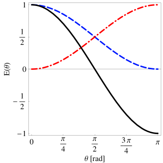
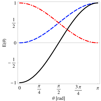
(a)	(b)
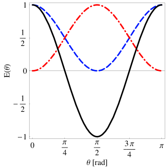
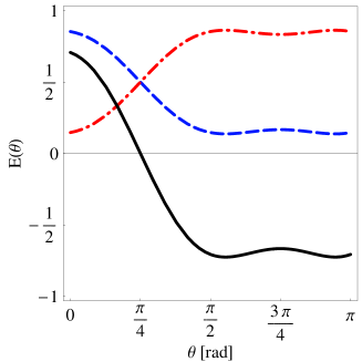
(c)	(d)
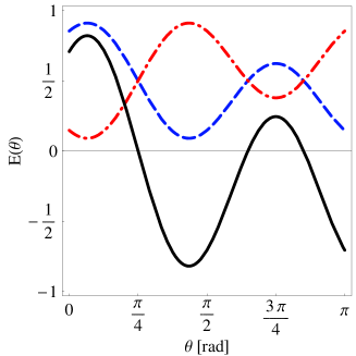
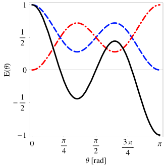
(e)	(f)

Figure 7: Probabilities and expectation values for (a) $\tau=0$, $\theta_{1}=\theta$, $\theta_{2}=\theta_{3}=\theta_{4}=0$, (b) $\tau=0$, $\theta_{1}=\theta$, $\theta_{2}=\theta_{3}=0$, $\theta_{4}=\pi$, (c) $\tau=\frac{\pi}{2}$, $\theta_{1}=\theta_{2}=-\theta_{3}=\theta_{4}=\theta$, (d) $\tau=\frac{\pi}{2}$, $\theta_{1}=-\theta_{3}=\theta_{4}=\theta$, $\theta_{2}=\frac{\pi}{4}$, (e) $\tau=\frac{\pi}{4}$, $\theta_{1}=-\theta_{3}=\theta_{4}=\theta$, $\theta_{2}=\frac{\pi}{4}$, (f) $\tau=\frac{\pi}{4}$, $\theta_{1}=-\theta_{3}=\theta_{4}=\theta$, $\theta_{2}=0$. Dashed (dash dotted) lines indicate probabilities to find an even (odd) number of “$-$” outcomes, solid lines depict expectation functions.

As there are four particles involved, the outcomes of one or two particles can be utilized to select the events of the other particles. Let “$\pm_{i}$” stand for the observation of spin state plus or minus on the $i$th particle. Table 6 contains the results of the associated expectation values and joint probabilities for finding an odd or even number of spin “$-$”-states.

Three-partite GHZM state (Ref. krenn1 )

$P_{\pm}={1\over 4}\left[1+2E\right]\;,\;P_{\pm}={1\over 4}\left[1-2E\right]\;,\;E_{\pm}=P_{\pm}-P_{\pm}$

$E_{\pm}(\theta_{1},\theta_{2},\theta_{3},\varphi_{1},\varphi_{2},\varphi_{3}|\pm_{3})=\frac{1}{2}\left[\cos\theta_{1}\cos\theta_{2}\pm_{3}\cos\left(\varphi_{1}+\varphi_{2}+\varphi_{3}\right)\sin\theta_{1}\sin\theta_{2}\sin\theta_{3}\right]$

Four-partite singlet states

$E_{\rho_{\Psi_{2,4,1}}}({\hat{\theta}},{\hat{\varphi}}|\pm_{4})=\frac{1}{12}\pm{1\over 2}E_{\rho_{\Psi_{2,4,1}}}({\hat{\theta}},{\hat{\varphi}})$

$E_{\rho_{\Psi_{2,4,1}}}({\hat{\theta}}|\pm_{3}\pm_{4})=\frac{1}{12}\left\{2(\pm_{3}1)(\pm_{4}1)\cos(\theta_{1}+\theta_{2}-\theta_{3}-\theta_{4})+\cos(\theta_{1}-\theta_{2})\left[1+(\pm_{3}1)(\pm_{4}1)\cos(\theta_{3}-\theta_{4})\right]\right\}$

$\begin{array}[]{lll}E_{\rho_{\Psi_{2,4,1}}}({\hat{\theta}},{\hat{\varphi}}|\pm_{3}\pm_{4})&=&\frac{1}{12}\left\{\cos\theta_{1}(2(\pm_{3}1)(\pm_{4}1)\sin\theta_{2}\left[\cos\theta_{4}\cos(\varphi_{2}-\varphi_{3})\sin\theta_{3}+\right.\right.\\ &&\qquad\left.\cos\theta_{3}\cos(\varphi_{2}-\varphi_{4})\sin\theta_{4}\right]+\\ &&\qquad\cos\theta_{2}\left[1+3(\pm_{3}1)(\pm_{4}1)\cos\theta_{3}\cos\theta_{4}-\right.\\ &&\qquad\left.(\pm_{3}1)(\pm_{4}1)\cos(\varphi_{3}-\varphi_{4})\sin\theta_{3}\sin\theta_{4}\right])+\\ &&\qquad\sin\theta_{1}(\cos(\varphi_{1}-\varphi_{2})\sin\theta_{2}\left[1-(\pm_{3}1)(\pm_{4}1)\cos\theta_{3}\cos\theta_{4}+\right.\\ &&\qquad\left.(\pm_{3}1)(\pm_{4}1)\cos(\varphi_{3}-\varphi_{4})\sin\theta_{3}\sin\theta_{4}\right]+\\ &&\qquad 2(\pm_{3}1)(\pm_{4}1)\left[\cos\theta_{2}\cos\theta_{4}\cos(\varphi_{1}-\varphi_{3})\sin\theta_{3}+\right.\\ &&\qquad\cos\theta_{2}\cos\theta_{3}\cos(\varphi_{1}-\varphi_{4})\sin\theta_{4}+\\ &&\qquad\left.\left.\left.\cos(\varphi_{1}+\varphi_{2}-\varphi_{3}-\varphi_{4})\sin\theta_{2}\sin\theta_{3}\sin\theta_{4}\right]\right)\right\}\end{array}$

$E_{\rho_{\Psi_{2,4,1}}}({\hat{\theta}}|\pm_{2}\pm_{4})=\frac{1}{12}\left\{(\pm_{2}1)(\pm_{4}1)\left[2\cos(\theta_{1}+\theta_{2}-\theta_{3}-\theta_{4})+\cos(\theta_{1}-\theta_{2})\cos(\theta_{3}-\theta_{4})\right]-2\cos(\theta_{1}-\theta_{3})\right\}$

$\begin{array}[]{lll}E_{\rho_{\Psi_{2,4,1}}}({\hat{\theta}},{\hat{\varphi}}|\pm_{2}\pm_{4})&=&\frac{1}{12}\left\{\cos\theta_{1}((\pm_{2}1)(\pm_{4}1)\sin\theta_{3}\left[2\cos\theta_{4}\cos(\varphi_{2}-\varphi_{3})\sin\theta_{2}-\right.\right.\\ &&\qquad\left.\cos\theta_{2}\cos(\varphi_{3}-\varphi_{4})\sin\theta_{4}\right]+\\ &&\qquad\cos\theta_{3}\left[-2+3(\pm_{2}1)(\pm_{4}1)\cos\theta_{2}\cos\theta_{4}+\right.\\ &&\qquad\left.2(\pm_{2}1)(\pm_{4}1)\cos(\varphi_{2}-\varphi_{4})\sin\theta_{2}\sin\theta_{4}\right])+\\ &&\qquad\sin\theta_{1}((\pm_{2}1)(\pm_{4}1)\cos\theta_{3}\left[-\cos\theta_{4}\cos(\varphi_{1}-\varphi_{2})\sin\theta_{2}+\right.\\ &&\qquad\left.2\cos\theta_{2}\cos(\varphi_{1}-\varphi_{4})\sin\theta_{4}\right]+\\ &&\qquad\sin\theta_{3}(2\left[-1+(\pm_{2}1)(\pm_{4}1)\cos\theta_{2}\cos\theta_{4}\right]\cos(\varphi_{1}-\varphi_{3})+\\ &&\qquad(\pm_{2}1)(\pm_{4}1)(2\cos(\varphi_{1}+\varphi_{2}-\varphi_{3}-\varphi_{4})+\\ &&\qquad\left.\cos(\varphi_{1}-\varphi_{2})\cos(\varphi_{3}-\varphi_{4}))\sin\theta_{2}\sin\theta_{4}))\right\}\end{array}$

Table 6: Probabilities and expectation functions for finding an odd or even number of spin “$-$”-states with selection. “$\pm_{i}$” stands for the observation of spin state plus or minus on the $i$th particle.

Two or three observables could also be grouped together to form a “condensed” observable. For instance, for each individual quadruple of outcomes $\{o_{1},o_{2},o_{3},o_{4}\}$ the values of the first and the second, as well as of the third and the fourth particle could be multiplied to obtain two other, dichotomic observables $o_{1}o_{2}$ and $o_{3}o_{4}$, respectively. More generally, one could take all partitions of 4, such that the outcomes of all particles within an element of the partition are multiplied. As the single outcomes occur at random, their resulting products and thus the new condensed observable would also represent random variables. Since the multiplication is associative, the resulting condensed correlations are just the four-partite correlations discussed so far.

V Summary

In summary, we have discussed an algorithmic procedure to enumerate all singlet states of $N$ particles of arbitrary spin. We have then explicitly enumerated the first cases for spin one-half and spin one and discussed their symmetries. These results have then be applied for a calculation of the quantum probabilities and expectation functions of four spin one-half particles in four arbitrary directions. We conclude by pointing out that all discussed configurations could, as a proof of principle, be locally realized by generalized beam splitters rzbb , zukowski-97 , svozil-2004-analog .

Dedication and acknowledgments: This paper is dedicated to Sylvia Pulmannova, in appreciation of her scientific accomplishments, and also for the enjoyment and privilege to be co-author in some of her research articles, as well as meeting her personally. One of the most remarkable impressions on me (K.S.) was her humbleness as a person and colleague, accompanied by her extreme professional skills in mathematics, logics and physics. The authors thank Rainer Dirl and Peter Kasperkovitz for their advise in group theoretical questions; K.S. gratefully acknowledges discussions with Boris Kamenik, Günther Krenn and Johann Summhammer in Viennese coffee houses and elsewhere.

References

-
[1]
K. Svozil, “Are simultaneous Bell measurements possible?” New Journal
of Physics 8, 39 (2006).
http://dx.doi.org/10.1088/1367-2630/8/3/039 -
[2]
A. Zeilinger, “A Foundational Principle for Quantum Mechanics,”
Foundations of Physics 29, 631–643 (1999).
http://dx.doi.org/10.1023/A:1018820410908 -
[3]
M. Eibl, S. Gaertner, M. Bourennane, C. Kurtsiefer, M. Zukowski, and
H. Weinfurter, “Experimental Observation of Four-Photon Entanglement
from Parametric Down-Conversion,” Physical Review Letters 90, 200 403
(2003).
http://dx.doi.org/10.1103/PhysRevLett.90.200403 - [4] A. Messiah, Quantum Mechanics, Vol. II (North-Holland, Amsterdam, 1962).
- [5] M. Chaichian and R. Hagedorn, Symmetries in Quantum Mechanics (Institute of Physics Publishing, Bristol and Philadelphia, 1998).
- [6] B. Wybourne, Symmetry Principles and Atomic Spectroscopy (Wiley Interscience, USA, 1970).
-
[7]
G. Krenn and A.Zeilinger, “Entangled entanglement,” Physical Review A
(Atomic, Molecular, and Optical Physics) 54, 1793–1797 (1996).
http://dx.doi.org/10.1103/PhysRevA.54.1793 - [8] L. E. Ballentine, Quantum Mechanics (Prentice Hall, Englewood Cliffs, NJ, 1989).
-
[9]
A. Einstein, B. Podolsky, and N. Rosen, “Can quantum-mechanical
description of physical reality be considered complete?” Physical Review 47, 777–780 (1935).
http://dx.doi.org/10.1103/PhysRev.47.777 -
[10]
K. Svozil, “On Counterfactuals and Contextuality,” in AIP
Conference Proceedings 750. Foundations of Probability and Physics-3,
A. Khrennikov, ed., pp. 351–360 (2005).
http://dx.doi.org/10.1063/1.1874586 - [11] R. D. Gill, “Time, Finite Statistics, and Bell’s Fifth Position,” in Proceedings of Foundations of Probability and Physics-2, A. Khrennikov, ed., pp. 179–206 (2003).
-
[12]
M. Reck, A. Zeilinger, H. J. Bernstein, and P. Bertani, “Experimental
realization of any discrete unitary operator,” Physical Review Letters 73, 58–61 (1994).
http://dx.doi.org/10.1103/PhysRevLett.73.58 -
[13]
M. Zukowski, A. Zeilinger, and M. A. Horne, “Realizable
higher-dimensional two-particle entanglements via multiport beam splitters,”
Physical Review A (Atomic, Molecular, and Optical Physics) 55,
2564–2579 (1997).
http://dx.doi.org/10.1103/PhysRevA.55.2564 -
[14]
K. Svozil, “Noncontextuality in multipartite entanglement,” J. Phys. A:
Math. Gen. 38, 5781–5798 (2005).
http://dx.doi.org/10.1088/0305-4470/38/25/013