Interplay of coupling and superradiant emission in the optical response of a double quantum dot

Abstract

We study theoretically the optical response of a double quantum dot structure to an ultrafast optical excitation. We show that the interplay of a specific type of coupling between the dots and their collective interaction with the radiative environment leads to very characteristic features in the time-resolved luminescence as well as in the absorption spectrum of the system. For a sufficiently strong coupling, these effects survive even if the transition energy mismatch between the two dots exceeds by far the emission line width.

I Introduction

Systems composed of two quantum dots (QDs) have attracted much attention in recent years. Many theoretical and experimental results have demonstrated that the physical properties of such double quantum dots (DQDs) are much richer than those of individual ones. On the one hand, this may pave the way to new applications, including long-time storage of quantum information pazy01b , conditional optical control unold05 that may lead to an implementation of a two-qubit quantum gate biolatti00 , generation of entangled photons gywat02 or coherent optical spin control and entangling troiani03 ; nazir04 ; gauger08b . On the other hand, in order to take advantage of these extended possibilities, the properties of DQDs have to be understood and controlled.

There are two major factors that determine the physical (in particular, optical) properties of DQDs: the coupling between the dots and their interaction with the environment. In both these areas new features appear, as compared to the physics of individual dots. Both problems have been in the focus of extensive experimental and theoretical work but many important questions remain open.

Coupling between the dots is essential for quantum conditional control, entanglement formation and implementation of two-qubit gates. It is therefore understandable that considerable experimental effort has been devoted to demonstrating its existence in double dot systems bayer01 ; ortner03 ; ortner05 ; ortner05b ; krenner05b , while theoretical studies were aimed at characterizing its signatures in the optical response of DQDs danckwerts06 .

Coupling of DQDs to their environment is affected by collective effects, which may lead to superradiance phenomena scheibner07 . Theoretical studies on the dephasing (in particular, decay of entanglement) in double dot systems have shown that coherence properties strongly depend on whether the dots are coupled to a common reservoir or to separate reservoirs yu02 ; yu03 ; tolkunov05 ; roszak06a . The collective nature of the coupling to the environment allows one to construct arrays (collective quantum bits) which are more resistant to decoherence than individual systems zanardi98b ; grodecka06 . In fact, in any such array of two-level systems collectively coupled to their common reservoir, the dephasing of some states is slowed down, while other states decohere faster. In the case of radiative decay, an essential role is played by the transition energy mismatch between the systems forming the array sitek07a . These subradiance and superradiance effects influence the optical response of DQDs and can affect the coherence properties of DQD-based quantum devices.

Since the paper by Dicke dicke54 , coherent effects in the radiative decay of two or more atoms have been studied in numerous works. The emission from identical stephen64 ; hutchinson64 ; lehmberg70a ; milonni74 ; agarwal74 and non-identical varfolomeev71 ; milonni75 two-level systems has been studied and methods suitable for the description of arrays of various shapes have been developed freedhoff04 ; rudolph04 . Systems formed by QDs share many features with those made of natural atoms. In particular, QD samples may be modelled as ensembles of two-level systems with parallel transition dipoles, corresponding to the fundamental optical (interband) transition between the ground (‘empty dot’) state and the confined exciton state (electron-hole pair in the dot), although one should not expect the transition energies to be exactly matched in these artificial objects. Nonetheless, these semiconductor structures are specific with some respects.

The spacing between QDs in intentionally manufactured DQD systems is typically of the order of nanometers, that is 2–3 orders of magnitude smaller than the wave length of the resonantly coupled radiation. This allows one to assume the Dicke limit of the coupling and neglect the retardation effects, which were one of the major concerns in the general theory milonni74 ; milonni75 . On the other hand, small distance between the two dots precludes individual addressing of each system by the exciting field so that only certain initial states may be prepared. This means, in particular, that the two-excitation (biexciton, i.e., one electron-hole pair in each QD of the DQD structure) states must be included in the description (except for the weak excitation limit).

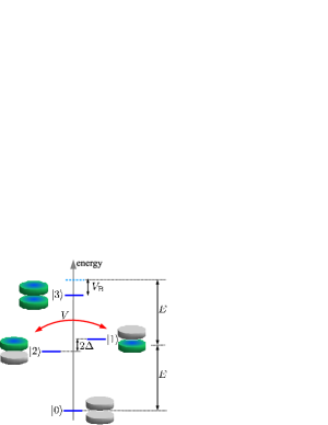
Figure 1: (Color online) Graphical representation of the energy levels (basis states) and couplings in the double quantum dot system.

Another important feature that distinguishes QDs from atomic samples is the presence of two kinds of dipole couplings. One of them is the direct interaction between static dipole moments associated with the electron-hole charge distribution in the two-dots unold05 . This kind of coupling is obviously present only if the two dots are occupied by excitons and its effect is to shift the energy of the biexciton state (denoted by $V_{\mathrm{B}}$ in Fig. 1). The other coupling is related to the interband matrix elements of the electric dipole moment and is analogous to the Förster coupling in molecular systems as well as to dipole couplings between atoms which appear in the description of superradiance phenomena in atomic samples. It couples the two single-exciton states of the system via a process that may be imagined as a recombination of the exciton in one of the dots with the subsequent transfer of energy to the other one (via Coulomb interaction), where the exciton is recreated (this coupling is denoted by $V$ in Fig. 1). Thus, this coupling has an “excitation transfer” character. In QDs, this interaction is modified by the finite size of the charge distribution (the QD size is comparable with the inter-dot distance) and has a finite value in the formal limit of vanishing distance govorov03 ; rozbicki08a ; machnikowski09a . Therefore, it is not a universal function of the distance. Finally, apart from this dipole-dipole coupling, other kinds of interaction may be present (e.g., effective ‘tunneling’ coupling accounting for a slight overlap of wave functions which may dominate over the Förster coupling for closely spaced dots). For these reasons, the strength of the coupling between the dots becomes an essentially independent parameter. All in all, there are three independent parameters governing the radiative properties of a double-dot system in the Dicke limit, compared to two in the case of atoms.

In this paper we study the interplay of all the factors affecting the optical response of a DQD: the coupling between the two dots forming the DQD, the mismatch between their transition energies and their collective interaction with the radiation environment (vacuum). With the recent experimental progress vamivakas09 ; flagg09 , optical studies of a single, resonantly driven nanostructure have become feasible. Therefore, we study the simplest optical property of the system, that is, the response to a single ultrafast pulse tuned to the fundamental interband transition of the system. The analysis includes the linear regime, where the spectral properties of the optical response yield the absorption spectrum of the system, as well as the higher order contributions which are affected by the exciton-biexciton dynamics. We show that both the time-resolved signal and its frequency spectrum can show clear signatures of collective coupling to the radiation reservoir. Moreover, in the realistic case of non-identical dots, the striking features related to collective radiative relaxation appear only when the inter-dot coupling is strong enough and has the “excitation transfer” character (as opposed to the occupation-preserving biexciton shift). In this way, our results provide a sensitive test for the appearance of a specific kind of coupling between the dots.

The paper is organized as follows. In Sec. II, we describe the system under study and define its model. In Sec. III, equations describing the evolution of the optical polarization are derived. Sec. IV contains the discussion of the results. Summary and final remarks are contained in Sec. V.

II The system

The system under study is a DQD composed of two QDs placed at a distance much smaller than the relevant photon wavelength. We restrict the discussion to the ground exciton states in the two dots. Due to strong electron-hole Coulomb attraction, the ‘spatially direct’ states (electron-hole pairs confined in the same dot) have much lower energy than the ‘dissociated’ states (we do not consider external electric fields which would change this picture szafran05 ; szafran08 ). Therefore, we include only the ‘spatially direct’ states in our model. We assume also that the polarization of the laser pulse corresponds to a polarization eigenstate of the excitons, which allows us to include only one out of the two bright states in each dot and to describe the DQD as a four level system, with the state $|0\rangle$ representing empty dots, $|1\rangle$ and $|2\rangle$ denoting the single exciton states with an exciton localized in the first and in the second dot, respectively, and $|3\rangle$ representing the “molecular biexciton” state, that is, the state with both dots occupied by an exciton. We denote the energies corresponding to the fundamental optical transition in the two dots by $E_{1,2}=E\pm\Delta$ and allow for a coupling between the dots, whose amplitude is $V$. The latter may originate either from the interband dipole (Förster) coupling between the dots danckwerts06 or appear as an effective description of tunnel coupling if the carrier wave functions in the two dots overlap. In addition, excitons confined in the two dots interact via their static dipole moments, which shifts the energy of the biexciton state by $V_{\mathrm{B}}$. The Hamiltonian describing the isolated DQD system is then

$$\tilde{H}_{\mathrm{X}} = (E+\Delta)|1\rangle\!\langle 1|+(E-\Delta)|2\rangle\!\langle 2|+(2E+V_{\mathrm{B}})|3\rangle\!\langle 3|$$

$$+V(|1\rangle\!\langle 2|+|2\rangle\!\langle 1|).$$

The structure of energy levels is shown in Fig. 1.

The two dots interact with their common radiative reservoir. The Hamiltonian describing this interaction is

$$\tilde{H}_{\mathrm{int}}=i\Sigma_{-}\sum_{\bm{k},\lambda}\bm{d}\cdot\hat{e}_{\lambda}\left(\bm{k}\right)\sqrt{\frac{\hbar\omega_{\bm{k}}}{2\epsilon_{0}\epsilon_{r}v}}b^{\dagger}_{\bm{k},\lambda}+\mathrm{H.c.},$$

with $\Sigma_{-}=\Sigma_{+}^{{\dagger}}=(\sigma^{\left(1\right)}_{-}+\sigma^{\left(2\right)}_{-})$, where $\sigma^{\left(1\right)}_{-}=|0\rangle\!\langle 1|+|2\rangle\!\langle 3|$ and $\sigma^{\left(2\right)}_{-}=|0\rangle\!\langle 2|+|1\rangle\!\langle 3|$ are annihilation operators for an exciton in the first and second dot, respectively, $\bm{k}$ is a photon wave vector, $\lambda$ denotes polarizations, $b_{\bm{k},\lambda},b_{\bm{k},\lambda}^{{\dagger}}$ are photon annihilation and creation operators, $\bm{d}$ is the interband dipole moment (for simplicity equal for both QDs), $\hat{e}_{\lambda}\left(\bm{k}\right)$ is a unit polarization vector, $\epsilon_{0}$ is the vacuum permittivity, $\epsilon_{\mathrm{r}}$ is the dielectric constant of the semiconductor, and $v$ is the normalization volume for the EM modes.

Finally,

$$H_{\mathrm{phot}}=\sum_{\bm{k},\lambda}\hbar\omega_{{\bm{k}}}b_{\bm{k},\lambda}^{{\dagger}}b_{\bm{k},\lambda}$$

is the Hamiltonian of the photon reservoir, where $\omega_{\bm{k}}$ is the frequency of the photon with a wave vector $\bm{k}$.

We will describe the evolution in a “rotating basis” defined by the unitary transformation

$$U=e^{iE(|1\rangle\!\langle 1|+|2\rangle\!\langle 2|+2|3\rangle\!\langle 3|)t/\hbar+iH_{\mathrm{phot}}t/\hbar}.$$

The transformed Hamiltonian is

$$H=U(\tilde{H}_{\mathrm{X}}+\tilde{H}_{\mathrm{int}}+H_{\mathrm{phot}})U^{{\dagger}}+i\hbar\frac{dU}{dt}U^{{\dagger}}=H_{\mathrm{X}}+H_{\mathrm{int}},$$

where

$$H_{\mathrm{X}}=\Delta(|1\rangle\!\langle 1|-|2\rangle\!\langle 2|)+V_{\mathrm{B}}|3\rangle\!\langle 3|+V(|1\rangle\!\langle 2|+|2\rangle\!\langle 1|)$$ (1)

and

$$H_{\mathrm{int}}=i\Sigma_{-}\sum_{\bm{k},\lambda}\bm{d}\cdot\hat{e}_{\lambda}\left(\bm{k}\right)\sqrt{\frac{\hbar\omega_{\bm{k}}}{2\epsilon_{0}\epsilon_{r}v}}e^{i\left(\omega_{\bm{k}}-E/\hbar\right)t}b^{\dagger}_{\bm{k},\lambda}+\mathrm{H.c.}$$

III The system evolution and the optical response

In this section we will describe the evolution of the DQD system after an instantaneous excitation with an ultrashort pulse. An analysis of both the time-resolved and spectrally-resolved response will be performed. In the linear response limit, the latter provides the linear susceptibility from which the absorption spectrum can be derived.

The source of the optical signal from the QD system is the electric dipole moment (polarization) related to the interband transition. Assuming identical magnitude and orientation of the transition dipoles in both dots, the relevant (interband) part of the dipole moment operator can be written as

$$\hat{\bm{d}}=\bm{d}\Sigma_{-}+\mathrm{H.c.}$$

The magnitude of the positive frequency part of the emitted coherent optical field, normalized to its initial value is, therefore,

$$P(t)=i\frac{\rho_{10}(t)+\rho_{20}(t)+\rho_{31}(t)+\rho_{32}(t)}{\rho_{10}(0)+\rho_{20}(0)+\rho_{31}(0)+\rho_{32}(0)},$$ (2)

where $\rho$ is the density matrix of the four-level DQD system and $\rho_{ij}(t)=\langle i|\rho(t)|j\rangle$. The matrix elements $\rho_{10}$ and $\rho_{20}$ are related to the coherences between the ground state and the single exciton states, hence are referred to as exciton polarizations. The other two matrix elements, $\rho_{31}$ and $\rho_{32}$, correspond to the transition between the single exciton and biexciton states and are commonly called biexciton polarizations.

An ultrafast pulse is assumed to be spectrally broad enough in order not to discriminate between the two dots in the structure. Due to a small (sub-wavelength) distance between the dots, they cannot be resolved spatially, either. Therefore, the pulse induces optical polarizations symmetrically and independently in both dots. After the pulse, the relevant elements of the density matrix have the values

$$\rho_{10}(0)=\rho_{20}(0) = -\frac{i}{2}\sin\alpha\cos^{2}\frac{\alpha}{2},$$ (3a)

$$\rho_{31}(0)=\rho_{32}(0) = -\frac{i}{2}\sin\alpha\sin^{2}\frac{\alpha}{2},$$ (3b)

where $\alpha$ is the pulse area.

After this instantaneous initial excitation, the density matrix evolves according to the Liouville–von Neumann–Lindblad equation of motion

$$\dot{\rho}=-\frac{i}{\hbar}\left[H_{\mathrm{X}},\rho\right]+\mathcal{L}[\rho],$$ (4)

with

$$\mathcal{L}[\rho]=\Gamma\left[\Sigma_{-}\rho\Sigma_{+}-\frac{1}{2}\{\Sigma_{+}\Sigma_{-},\rho\}_{+}\right],$$ (5)

where

$$\Gamma=\frac{E^{3}|\bm{d}|^{2}\sqrt{\epsilon_{\mathrm{r}}}}{3\pi\epsilon_{0}c^{3}\hbar^{4}}$$

is the spontaneous decay rate. It can be noted that, from the formal point of view, the evolution equation (4) is not unique. In fact, a standard microscopic derivation breuer02 involves grouping the transitions into sets characterized by the values of the transition energies and, therefore, produces two different Lindblad equations, depending on the arbitrary classification of the two radiating systems as “identical” or “different”. Therefore, it does not provide any means for the study of the transition from the independent decay to the collective regime as the transition energy mismatch $\Delta$ is varied from zero to a finite value. On the other hand, Eq. (4), composed of the unitary and dissipative parts, is compatible with the Wigner-Weisskopf description of the double QD system varfolomeev71 ; sitek07a , where the Markov approximation is performed without any arbitrariness (assuming $\Delta\ll E$, so that the reservoir spectral density does not vary considerably over the relevant frequency range).

Note that the collective coupling of the two dots to the electromagnetic field, as described by Eq. (5), results in the appearance of cross-terms of the form $\sigma_{-}^{(i)}\rho\sigma_{+}^{(j)}$, $i\neq j$, which are absent in the case of individual coupling to separate reservoirs (see Appendix). These terms correspond to the imaginary part of the coupling that appears in other approaches varfolomeev71 ; freedhoff04 ; rudolph04 . Thus, in the limit of vanishing biexciton shift and (in the case of Refs. freedhoff04, ; rudolph04, ) of identical dots, our model is fully equivalent to the small-system limit of those theories.

The equation of motion (4) leads to the closed system of four equations for the matrix elements of interest,

$$\dot{\rho}_{10} = \left(-i\frac{\Delta}{\hbar}-\frac{\Gamma}{2}\right)\rho_{10}+\left(-i\frac{V}{\hbar}-\frac{\Gamma}{2}\right)\rho_{20}$$ (6a)

$$+\Gamma(\rho_{31}+\rho_{32}),$$

$$\dot{\rho}_{20} = \left(-i\frac{V}{\hbar}-\frac{\Gamma}{2}\right)\rho_{10}+\left(i\frac{\Delta}{\hbar}-\frac{\Gamma}{2}\right)\rho_{20}$$ (6b)

$$+\Gamma(\rho_{31}+\rho_{32}),$$

$$\dot{\rho}_{32} = \left(-i\frac{V_{\mathrm{B}}}{\hbar}-i\frac{\Delta}{\hbar}-\frac{3\Gamma}{2}\right)\rho_{32}$$ (6c)

$$+\left(i\frac{V}{\hbar}-\frac{\Gamma}{2}\right)\rho_{31},$$

$$\dot{\rho}_{31} = \left(i\frac{V}{\hbar}-\frac{\Gamma}{2}\right)\rho_{32}$$ (6d)

$$+\left(-i\frac{V_{\mathrm{B}}}{\hbar}+i\frac{\Delta}{\hbar}-\frac{3\Gamma}{2}\right)\rho_{31}.$$

This system of equations with the initial values given by Eqs. (3a-b) can be solved by the standard Laplace transform method. Then, for the total emitted signal [Eq. (2)], we find

$$P(t)=\frac{i}{2}\sum_{i}\left[\cos^{2}\frac{\alpha}{2}A_{i}+\sin^{2}\frac{\alpha}{2}B_{i}\right]e^{\lambda_{i}t},$$ (7)

where (with the first index corresponding to the upper sign)

$$\lambda_{1,2} = \pm i\tilde{\Omega}_{-}-\frac{\Gamma}{2},$$ (8a)

$$\lambda_{3,4} = i(\pm\tilde{\Omega}_{+}-V_{\mathrm{B}}/\hbar)-\frac{3\Gamma}{2},$$ (8b)

$$A_{1,2} = 1\mp\frac{V/\hbar-i\Gamma/2}{\tilde{\Omega}_{-}},$$ (8c)

$$B_{1,2} = \frac{\mp 2\Gamma V_{\mathrm{B}}\tilde{\Omega}_{-}+2\Gamma V_{\mathrm{B}}V/\hbar-i\Gamma^{2}V_{\mathrm{B}}-2\Delta^{2}\Gamma/\hbar}{\tilde{\Omega}_{-}[\mp 2\Gamma V-(iV_{\mathrm{B}}+\hbar\Gamma)(2\tilde{\Omega}_{-}\pm V_{\mathrm{B}}/\hbar\mp i\Gamma)]},$$ (8d)

$$A_{3,4} = 0,$$ (8e)

$$B_{3,4} = \frac{\pm(V_{\mathrm{B}}/\hbar-2i\Gamma)(2iV-iV_{\mathrm{B}}+\hbar\Gamma)+2iV_{\mathrm{B}}\tilde{\Omega}_{-}}{(iV_{\mathrm{B}}+\hbar\Gamma)(2\tilde{\Omega}_{+}\mp V_{\mathrm{B}}/\hbar\pm i\Gamma)\pm 2\Gamma V}$$ (8f)

$$+\frac{4\Gamma V^{2}/\hbar-iV_{\mathrm{B}}^{2}V/\hbar^{2}+\Gamma V_{\mathrm{B}}^{2}/(2\hbar)+\hbar\Gamma^{3}}{\tilde{\Omega}_{+}[(iV_{\mathrm{B}}+\hbar\Gamma)(2\tilde{\Omega}_{+}\mp V_{\mathrm{B}}/\hbar\pm i\Gamma)\pm 2\Gamma V]},$$

with

$$\tilde{\Omega}_{\pm}=\sqrt{(V/\hbar)^{2}\pm iV\Gamma/\hbar-\Gamma^{2}/4+(\Delta/\hbar)^{2}}.$$ (9)

The Fourier transform of this signal is

$$\hat{P}(\omega)=\frac{\cos^{2}\frac{\alpha}{2}f(\omega)+\sin^{2}\frac{\alpha}{2}g(\omega)}{(\omega-i\lambda_{1})(\omega-i\lambda_{2})(\omega-i\lambda_{3})(\omega-i\lambda_{4})},$$ (10)

where

$$f(\omega)=i(\omega+V/\hbar)(\omega-i\lambda_{3})(\omega-i\lambda_{4})$$ (11)

and

$$g(\omega) = i(\omega-V_{\mathrm{B}}/\hbar-V/\hbar+3i\Gamma)(\omega-i\lambda_{1})(\omega-i\lambda_{2})$$

$$+2\Gamma V_{\mathrm{B}}(V/\hbar+\omega)/\hbar-2\Delta^{2}\Gamma/\hbar^{2}.$$

It should be noted that the frequency $\omega$ in the above equations (and in the following discussion) is defined with respect to the mean transition frequency, that is, $\omega=\tilde{\omega}-E/\hbar$, where $\tilde{\omega}$ is the actual frequency of the emitted electromagnetic radiation.

IV Discussion

The evolution of the optical polarization after an instantaneous excitation depends on whether the dots are coupled or not. In this section we will discuss the two cases, comparing the optical response of the two dots interacting with the common reservoir in the Dicke limit (separation of the dots is small compared to $\hbar c/E$), using the solution derived in Sec. III, with the response of a hypothetical system consisting of two dots interacting with independent reservoirs.

IV.1 Uncoupled dots

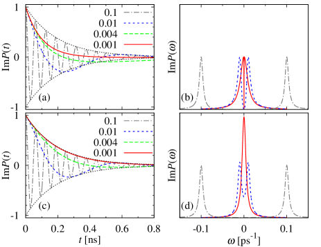
Figure 2: (Color online) (a,c) The optical polarization as a function of time after an ultrafast excitation for uncoupled dots ($V=V_{\mathrm{B}}=0$) in the linear response limit ($\alpha\to 0$). (b,d) The corresponding spectrum. Figs. (a,b) show the results for QDs interacting with a common reservoir in the Dicke limit, while Figs. (c,d) refer to dots radiating into independent reservoirs. Here $\Gamma=0.01$ ps^-1 and the values of $\Delta/\hbar$ are as shown in the figure (in ps^-1). Line definitions in (b,d) are the same as in (a,c). Dotted lines in (a,c) show the envelope $\pm\exp(-\Gamma t/2)$. The vertical scale in (b) and (d) is the same.

In the case of uncoupled QDs ($V=V_{\mathrm{B}}=0$) the optical response is determined by the interplay of the other two parameters: the recombination rate $\Gamma$ and the transition energy mismatch $\Delta$. In Fig. 2 we show the optical polarization in the time and frequency domain for a fixed value of the radiative recombination time $1/\Gamma=100$ ps. We assume here $\alpha\to 0$ (linear response limit), so that the imaginary part of the Fourier transform of the normalized signal is proportional to the absorption spectrum of the DQD. In this case, $P(t)$ is purely imaginary.

For $\Delta\gg\hbar\Gamma$ the evolution of the optical signal is dominated by optical beats due to the interference of fields emitted from the two dots [Fig. 2(a,c), gray dash-dotted line]. There is no noticeable difference between the cases of a common reservoir [Fig. 2(a)] and separate reservoirs [Fig. 2(c)]. This is not surprising since systems with different transition energies emit into different frequency sectors of the reservoir and thus essentially interact with different reservoirs anyway. The two spectra [Fig. 2(b,d)] also look indistinguishable in this case.

This situation changes as the energy mismatch $\Delta$ is decreased (Fig. 2, blue and green dashed lines). One effect, which follows from Eqs. (8a) and (9), is that the frequency is decreased in the collective case, although this does not lead to any qualitative difference in the evolution of the optical polarization represented in the time domain [Fig. 2(a,c)]. A much more pronounced difference is visible in the spectra [Fig. 2(b,d)]. From Eqs. (10) and (11) one has in the present special case, for $\Delta>\hbar\Gamma/2$

$$\operatorname{Im}P(\omega|\alpha=0,V=0,\Delta>\hbar\Gamma/2)=$$

$$\frac{\Gamma\omega/\Omega_{+}}{4(\omega-\Omega_{+})^{2}+\Gamma^{2}/4}-\frac{\Gamma\omega/\Omega_{+}}{4(\omega+\Omega_{+})^{2}+\Gamma^{2}/4},$$

where $\Omega_{+}=\sqrt{(\Delta/\hbar)^{2}-\Gamma^{2}/4}$. This takes the form of two Lorentzians centered around $\omega=\pm\Omega_{+}$ only as long as $\Gamma/\Omega_{+}$ is small and only for $|\omega-\Omega_{+}|\lesssim\Gamma$. In fact, $P(\omega=0)=0$, which means that the spectrum must considerably differ from the sum of two Lorentzians when the latter overlap. This can be seen in Figs. 2(b,d) (blue dashed line).

The particular features of the DQD spectrum in the common reservoir case become even more pronounced when $\Delta<\hbar\Gamma/2$. Now $\Omega_{+}$ is imaginary and the absorption spectrum can be written as

$$\operatorname{Im}P(\omega|\alpha=0,V=0,\Delta<\hbar\Gamma/2)=$$

$$\frac{\Gamma_{+}}{|\Omega_{+}|}\frac{\Gamma_{+}}{4\omega^{2}+\Gamma_{+}^{2}}-\frac{\Gamma_{-}}{|\Omega_{+}|}\frac{\Gamma_{-}}{4\omega^{2}+\Gamma_{-}^{2}},$$

where $\Gamma_{\pm}=\Gamma\pm 2|\Omega_{+}|$. Since $\Gamma_{+}\to 2\Gamma$ as $\Delta\to 0$, the width of the first Lorentzian becomes twice larger than it was for independent reservoirs. This term corresponds to the superradiant component of the system evolution sitek07a . The second Lorentzian (which is negative) becomes narrow, since $\Gamma_{-}\to 0$ as $\Delta\to 0$, and represents the subradiant component. However, its weight vanishes in the limit of identical dots [note that the amplitudes of the two Lorentzians are always exactly opposite, in accordance with $P(\omega=0)=0$]. These spectral features are reflected by the evolution in the time domain shown in Fig. 2(a). For $\Delta$ slightly below $\hbar\Gamma/2$ (green long dashed line), the evolution is a sum of two exponential factors: one positive, large, and short living and the other one negative, small, and long living. In fact, however, the resulting behavior is hardly distinguishable from the strongly damped oscillations appearing for individually emitting dots [Fig. 2(c)]. Only for $\Delta\ll\hbar\Gamma$ the difference becomes remarkable: in the case of collective emission, the polarization becomes dominated by the superradiant component which leads to a decay with a doubled rate, as compared to the separate reservoir case [red solid lines in Figs. 2(a,c)].

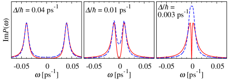
Figure 3: (Color online) The transition from the ‘different dots’ regime to the ‘identical dots’ regime as manifested by the form of the absorption spectrum of a DQD system. Here $\Gamma=0.01$ ps^-1 and the values of $\Delta/\hbar$ are shown in the figures. Red solid lines: the actual system; blue dashed lines: hypothetical system made of two dots interacting with separate reservoirs.

These results allow one to understand the transition from the limit of different systems (separate reservoirs) to identical systems (common reservoir). This transition is manifested in the reconstruction of the absorption spectrum, as shown in Fig. 3. As long as $\Delta\gg\hbar\Gamma/2$, the two dots are coupled to different frequency sectors of the electromagnetic reservoir and the spectrum of the DQD system is almost indistinguishable from that of two dots coupled to separate reservoirs. In the most interesting parameter range, $\Delta\sim\hbar\Gamma/2$, the spectrum is non-Lorentzian as long as $\Delta>\hbar\Gamma/2$ and then switches to an unusual form of two Lorentzians with different weights and opposite signs, centered at zero frequency. Only then the evolution of polarization has two exponentially decaying components.

Although the features discussed above are interesting from a general physical point of view, their appearance requires that the energy mismatch between the dots is comparable with the radiative line width, that is, of the order of tens of $\mu$eV. In spite of the rapid progress of nanostructure manufacturing, this can be very hard to achieve experimentally, unless the dots can be driven to resonance by external fields (e.g. taking advantage of a different strength of the DC Stark effect in the two dots). As we will show in Sec. IV.3, if the dots are coupled by an “excitation transfer” interaction, the collective effects manifest themselves already for much larger values of the energy mismatch. Before we proceed to this case, we study the effect of the other type of long-range interaction between confined excitons which is due to static electric dipoles and results in a biexciton shift.

IV.2 Coupled dots: Biexciton shift

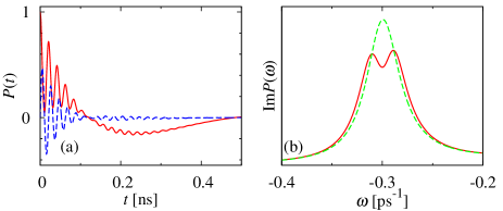
Figure 4: (Color online) (a) The optical polarization as a function of time after an ultrafast excitation for dots coupled by the static dipole moments only ($V=0$, $V_{\mathrm{B}}\neq 0$) for $\tan^{2}(\alpha/2)=0.2$, $\Gamma=0.01$ ps^-1, $\Delta/\hbar=0.01$ ps^-1, $V_{\mathrm{B}}/\hbar=-0.3$ ps^-1. Blue dashed line: real part, red solid line: imaginary part. (b) The Fourier transform of the polarization signal. Red solid line: parameters as in (a). Green dashed line: $\Delta/\hbar=0.001$ ps^-1.

In this section we discuss the evolution of the optical polarization for a system of two QDs coupled by a static dipole interaction $V_{\mathrm{B}}$ (we keep $V=0$). This coupling is important only for the third (and higher) order terms in the optical signal. In the parameter range where the transition between the two regimes of evolution occurs, as discussed in Sec. IV.1, the biexciton shift $V_{\mathrm{B}}$ (which is of the order of meV) is likely to be the largest energy scale of the problem. Therefore, we restrict the discussion to the case of $V_{\mathrm{B}}\gg\Delta$ and $V_{\mathrm{B}}\gg\hbar\Gamma$. Then, from Eq. (8d), in the leading order, $B_{1,2}\sim\hbar\Gamma/V_{\mathrm{B}}$, which means that the correction to the components evolving with the frequencies $i\lambda_{1}$ and $i\lambda_{2}$, as well as to the spectrum of the optical response in the frequency range studied in Sec. IV.1, is negligible.

In the spectral region of $\omega\sim V_{\mathrm{B}}/\hbar$, a new feature appears when $V_{\mathrm{B}}\neq 0$ [see Fig. 4(b)]. The shape of this feature evolves in a different way, as compared to the absorption line at $\omega=0$. For $\Delta\gg\hbar\Gamma$ two nearly Lorentzian lines of almost equal magnitude appear at $\omega=(V_{\mathrm{B}}\pm\Delta)/\hbar$. These two lines collapse as $\Delta\sim\hbar\Gamma$ but in this case they retain their approximately Lorentzian shape. For $\Delta<\hbar\Gamma/2$ both Lorentzians are centered at the same frequency $\omega=V_{\mathrm{B}}/\hbar$, as in the absorption spectrum discussed above, but now their widths tend to $\Gamma$ and $2\Gamma$ as $\Delta\to 0$. The area of the narrower line (which is negative) vanishes in this limit which, in view of the finite width, implies that the amplitude of this line vanishes. On the other hand, the area of the broader line remains finite. This means that the evolution of the biexciton beats [presented in Fig. 4(a)] shows a two-rate damping which becomes dominated by the short-living component as the dots become identical. In contrast, as follows from the formulas listed in the Appendix, in the case of independent reservoir the polarization decay rate is always $3\Gamma/2$.

IV.3 Coupled dots: transfer interaction

In this section we consider the case of two dots coupled by an “excitation transfer” interaction, that is, $V\neq 0$ in Eq. (1). We assume that the magnitude of this coupling is larger than the relaxation rate, $V\gg\hbar\Gamma$. As we will see, values of the energy mismatch $\Delta$ for which the transition to the collective behavior takes place is now of the order of $V$ so that $\Gamma$ becomes the smallest frequency in the problem. One can, therefore, simplify the discussion by retaining only the terms up to linear order in $\Gamma$ in Eqs. (8a,b) and taking the amplitudes given by Eqs. (8c-f) at $\Gamma=0$.

Then one gets $\lambda_{1,2}=\pm i\Omega-\Gamma_{\mp}/2$ and $A_{1,2}=1\mp V/(\hbar\Omega)$, where $\Gamma_{\mp}=[1\mp V/(\hbar\Omega)]\Gamma$, $\Omega=[\Delta^{2}+V^{2}]^{1/2}/\hbar$. Thus, in the linear response limit, the system shows a decay described by two exponential components. The subradiant one decays with the rate $\Gamma_{-}/2<\Gamma/2$ and its amplitude vanishes when $\Delta\ll V$. The decay rate of the superradiant component is $\Gamma_{+}/2>\Gamma/2$. This component dominates the decay in the limit of strongly coupled dots.

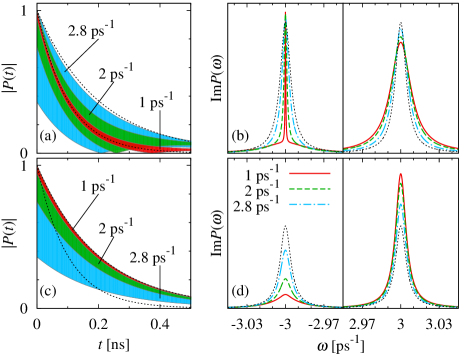
Figure 5: (Color online) Left panels: envelope of the optical beats for two coupled QDs emitting to a common reservoir and to separate reservoirs. For each value of $\Delta/\hbar$ (shown in the plot), the coupling $V$ is adjusted so that $\Omega=3$ ps^-1 in each case. Right panels: the corresponding absorption spectra. Plots (a) and (b) show the properties of a DQD emitting to a common reservoir, while plots (c,d) correspond to two dots emitting to separate reservoirs. Dotted lines in (a,c) show exponential decay curves with the rates $\Gamma/2$ and $\Gamma$, while in (b,d) they show Lorentzians of equal weight and width $\Gamma/2$.

The evolution of the optical polarization in the present case is shown in Fig. 5(a), where we plot the envelopes of the optical beats for three different sets of parameters $\Delta$ and $V$. Two effects that may be noticed are the decrease of the beating amplitude and the change in the decay rate of the signal as the energy mismatch decreases and the coupling increases. By comparison with the case of independent reservoirs [Fig. 5(c)] one can see that the first of these two effects appears in both cases. A non-selective excitation induces a symmetric superposition of the two occupations which has a larger overlap with one of the eigenstates of the coupled dots. Therefore, one of the oscillators contributing to the beats has a larger amplitude and the beating amplitude is reduced.

In contrast, the other effect is related to the collective interaction with the photon reservoir. In the physical case of a common reservoir, the eigenstate dominating the response is the superradiant one. In the limit of $\Delta\to 0$ only the superradiant state is excited (it coincides with the optically active symmetric superposition). This is reflected by the decay of the optical response, as shown in Fig. 5(a). For $\Delta\gg V$, the optical polarization decays with the rate $\Gamma/2$, characteristic of a single system. As the coupling $V$ becomes comparable with the energy mismatch $\Delta$, the decay becomes non-exponential and, in fact, contains two components decaying with different rates. When the coupling dominates over the energy mismatch, $V\gg\Delta$, the subradiant component vanishes and the signal decays with the doubled rate $\Gamma$. On the contrary, hypothetical dots coupled to independent reservoirs [Fig. 5(c)] always show a decay of the optical response with the same rate $\Gamma/2$.

The absorption spectrum corresponding to the time-resolved response discussed above is shown in Figs. 5(b,d). The two models of common and separate reservoirs differ essentially. In both cases there is a similar transfer of line weight from one line to the other as the energy mismatch decreases and the coupling increases. However, the way the line shapes change is very different. In the case of independent reservoirs [Fig. 5(d)], the line widths remain constant (no sub- and superradiance effects) and only the line amplitudes change. On the contrary, when the dots are coupled to a common reservoir, the amplitudes of the lines are almost constant but their widths change. This is quite a remarkable signature of the joint appearance of inter-dot coupling and collective radiative decoherence in the system. It is also interesting to note that, since the weights of each line behaves almost in the same way in both cases, no difference can be observed if the absorption is averaged over an inhomogeneous ensemble.

V Conclusions

We have shown that the coexistence of coupling between quantum dots and collective effects in their interaction with the electromagnetic environment leaves clear traces in the optical response of these systems.

For uncoupled dots, the collective radiative properties (sub- and superradiance) become important only when the energy mismatch falls below the absorption line width. The decay of the polarization then evolves from damped oscillations (beats) for different dots to a superradiant exponential decay for identical dots. For very similar dots the corresponding absorption line is composed of two Lorentzians superposed at the same transition frequency, with the same amplitude but different widths and opposite signs.

Coupling between the dots changes this picture considerably. Now superradiance effects can be observed as long as the energy mismatch is smaller or comparable to the coupling strength. The envelope of the optical beats in this case decays with the usual rate for different dots and with the double (superradiant) rate when the coupling becomes much larger than the energy mismatch. In the intermediate range, the decay is composed of two exponential components.

These effects in the time-resolved optical response are reflected in the absorption spectrum, where the lines corresponding to the small and large components in the optical response loose or gain, respectively, their widths (reflecting the sub- and superradiance property). This presents a clear difference with respect to the (hypothetical) case of dots emitting to different reservoirs where the lines loose or gain amplitude, while their widths remain constant. This essentially different form of absorption lines which, for sufficiently strongly coupled dots, can be observed even for a transition energy mismatch in the range of milli-electron-volts provides an experimentally accessible signature of coupling and collective decoherence in double quantum dots.

Appendix A Radiative decay to independent reservoirs

In this appendix, we derive the equations of motion for the optical polarizations and find the resulting optical response in the case of a two coupled QDs interacting with separate photon reservoirs.

The initial values for the relevant matrix elements (at $t=0$) are given by Eqs. (3a,b). At $t>0$, the density matrix evolves according to Eq. (4) but the Lindblad operator now has the form

$$\mathcal{L}[\rho]=\sum_{i=1,2}\Gamma\left[\sigma^{(i)}_{-}\rho\sigma^{(i)}_{+}-\frac{1}{2}\{\sigma^{(i)}_{+}\sigma^{(i)}_{-},\rho\}_{+}\right].$$

This equation corresponds to the system of evolution equations for the optical coherences

$$\dot{\rho}_{10} = \left(-i\Delta/\hbar-\Gamma/2\right)\rho_{10}-i(V/\hbar)\rho_{20}+\Gamma\rho_{32},$$

$$\dot{\rho}_{20} = -i(V/\hbar)\rho_{10}+\left(i\Delta/\hbar-\Gamma/2\right)\rho_{20}+\Gamma\rho_{31},$$

$$\dot{\rho}_{32} = \left(-iV_{\mathrm{B}}/\hbar-i\Delta/\hbar-3\Gamma/2\right)\rho_{32}+i(V/\hbar)\rho_{31},$$

$$\dot{\rho}_{31} = i(V/\hbar)\rho_{32}+\left(-iV_{\mathrm{B}}/\hbar+i\Delta/\hbar-3\Gamma/2\right)\rho_{31}.$$

By solving this system of equations one finds the normalized optical polarization defined by Eq. (7) with

$$\lambda_{1,2}=\pm i\Omega-\frac{\Gamma}{2},\quad\lambda_{3,4}=i(\pm\Omega-V_{\mathrm{B}}/\hbar)-\frac{3\Gamma}{2},$$

$$A_{1,2}=1\mp\frac{V}{\hbar\Omega},\quad A_{3,4}=0,$$

$$B_{1,2}=\frac{\Gamma[(V_{\mathrm{B}}/\hbar-i\Gamma)(\mp\Omega+V/\hbar)-2\Delta^{2}/\hbar^{2}]}{2\Omega[(-iV_{\mathrm{B}}/\hbar-\Gamma)(\pm V_{\mathrm{B}}/\hbar\mp i\Gamma+2\Omega)]},$$

$$B_{3,4}=\frac{(iV_{\mathrm{B}}+\hbar\Gamma)(V_{\mathrm{B}}-2V)(V/\hbar\pm\Omega)+2\Delta^{2}V_{\mathrm{B}}/\hbar}{\Omega(iV_{\mathrm{B}}+\hbar\Gamma)(\pm V_{\mathrm{B}}\mp i\hbar\Gamma-2\hbar\Omega)},$$

where $\Omega=\sqrt{V^{2}+\Delta^{2}}/\hbar$.

The Fourier transform of this signal is

$$P(\omega)=\frac{\cos^{2}\frac{\alpha}{2}f(\omega)+\sin^{2}\frac{\alpha}{2}g(\omega)}{(\omega-i\lambda_{1})(\omega-i\lambda_{2})(\omega-i\lambda_{3})(\omega-i\lambda_{4})},$$

where $f(\omega)=i(\omega+V/\hbar+i\Gamma/2)(\omega-i\lambda_{3})(\omega-i\lambda_{4})$ and

$$g(\omega) = i(\omega-V/\hbar-V_{\mathrm{B}}/\hbar+5i\Gamma/2)(\omega-i\lambda_{1})(\omega-i\lambda_{2})$$

$$+\Gamma(\omega+V/\hbar+i\Gamma/2)(V_{\mathrm{B}}/\hbar-i\Gamma)-2\Delta^{2}\Gamma/\hbar^{2}.$$

References

- (1) E. Pazy, I. D’Amico, P. Zanardi, and F. Rossi, Phys. Rev. B 64, 195320 (2001).
- (2) T. Unold, K. Mueller, C. Lienau, T. Elsaesser, and A. D. Wieck, Phys. Rev. Lett. 94, 137404 (2005).
- (3) E. Biolatti, R. C. Iotti, P. Zanardi, and F. Rossi, Phys. Rev. Lett. 85, 5647 (2000).
- (4) O. Gywat, G. Burkard, and D. Loss, Phys. Rev. B 65, 205329 (2002).
- (5) F. Troiani, E. Molinari, and U. Hohenester, Phys. Rev. Lett. 90, 206802 (2003).
- (6) A. Nazir, B. W. Lovett, S. D. Barrett, T. P. Spiller, and G. A. D. Briggs, Phys. Rev. Lett. 93, 150502 (2004).
- (7) E. M. Gauger, A. Nazir, S. C. Benjamin, T. M. Stace, and B. W. Lovett, New J. Phys. 10, 073016 (2008).
- (8) M. Bayer, P. Hawrylak, K. Hinzer, S. Fafard, M. Korkusinski, Z. R. Wasilewski, O. Stern, and A. Forchel, Science 291, 451 (2001).
- (9) G. Ortner, M. Bayer, A. Larionov, V. B. Timofeev, A. Forchel, Y. B. Lyanda-Geller, T. L. Reinecke, P. Hawrylak, S. Fafard, and Z. Wasilewski, Phys. Rev. Lett. 90, 086404 (2003).
- (10) G. Ortner, I. Yugova, G. Baldassarri Höger von Högersthal, A. Larionov, H. Kurtze, D. R. Yakovlev, M. Bayer, S. Fafard, Z. Wasilewski, P. Hawrylak, Y. B. Lyanda-Geller, T. L. Reinecke, A. Babinski, M. Potemski, V. B. Timofeev, and A. Forchel, Phys. Rev. B 71, 125335 (2005).
- (11) G. Ortner, M. Bayer, Y. Lyanda-Geller, T. L. Reinecke, A. Kress, J. P. Reithmaier, and A. Forchel, Phys. Rev. Lett. 94, 157401 (2005).
- (12) H. J. Krenner, M. Sabathil, E. C. Clark, A. Kress, D. Schuh, M. Bichler, G. Abstreiter, and J. J. Finley, Phys. Rev. Lett. 94, 057402 (2005).
- (13) J. Danckwerts, K. J. Ahn, J. Förstner, and A. Knorr, Phys. Rev. B 73, 165318 (2006).
- (14) M. Scheibner, T. Schmidt, L. Worschech, A. Forchel, G. Bacher, T. Passow, and D. Hommel, Nature Physics 3, 106 (2007).
- (15) T. Yu and J. H. Eberly, Phys. Rev. B 66, 193306 (2002).
- (16) T. Yu and J. H. Eberly, Phys. Rev. B 68, 165322 (2003).
- (17) D. Tolkunov, V. Privman, and P. K. Aravind, Phys. Rev. A 71, 060308(R) (2005).
- (18) K. Roszak and P. Machnikowski, Phys. Rev. A 73, 022313 (2006).
- (19) P. Zanardi and F. Rossi, Phys. Rev. Lett. 81, 4752 (1998).
- (20) A. Grodecka and P. Machnikowski, Phys. Rev. B 73, 125306 (2006).
- (21) A. Sitek and P. Machnikowski, Phys. Rev. B 75, 035328 (2007).
- (22) R. H. Dicke, Phys. Rev. 93, 99 (1954).
- (23) M. J. Stephen, J. Chem. Phys. 40, 669 (1964).
- (24) D. A. Hutchinson and H. F. Hameka, J. Chem. Phys. 41, 2006 (1964).
- (25) P. W. Milonni and P. L. Knight, Phys. Rev. A 10, 1096 (1974).
- (26) R. H. Lehmberg, Phys. Rev. A 2, 883 (1970).
- (27) G. S. Agarwal, Quantum Statistical Theories of Spontaneous Emission and their Relation to Other Approaches, Vol. 70 of Springer tracts in modern physics, G. Höhler (Ed.) (Springer, Berlin, 1974).
- (28) A. Varfolomeev, Zh. Eksp. Teor. Fiz. 59, 1702 (1970) [Sov. Phys.–JETP 32, 926 (1971)].
- (29) P. W. Milonni and P. L. Knight, Phys. Rev. A 11, 1090 (1975).
- (30) H. Freedhoff, Phys. Rev. A 69, 013814 (2004).
- (31) T. Rudolph, I. Yavin, and H. Freedhoff, Phys. Rev. A 69, 013815 (2004).
- (32) A. O. Govorov, Phys. Rev. B 68, 075315 (2003).
- (33) E. Rozbicki and P. Machnikowski, Phys. Rev. Lett. 100, 027401 (2008).
- (34) P. Machnikowski and E. Rozbcki, Phys. Stat. Sol. (b) 246, 320 (2009).
- (35) A. N. Vamivakas, Y. Zhao, C.-Y. Lu, and M. Atatüre, Nature Physics 5, 198 (2009).
- (36) E. B. Flagg, A. Muller, J. W. Robertson, S. Founta, D. G. Deppe, M. Xiao, W. Ma, G. J. Salamo, and C. K. Shih, Nature Physics 5, 203 (2009).
- (37) B. Szafran, T. Chwiej, F. M. Peeters, S. Bednarek, J. Adamowski, and B. Partoens, Phys. Rev. B 71, 205316 (2005).
- (38) B. Szafran, Acta Phys. Polon. A 114, 1013 (2008).
- (39) H.-P. Breuer and F. Petruccione, The Theory of Open Quantum Systems (Oxford University Press, Oxford, 2002).