The Density of Coronal Null Points from Hinode and MDI

Abstract

Magnetic null points can be located numerically in a potential field extrapolation or their average density can be estimated from the Fourier spectrum of a magnetogram. We use both methods to compute the null point density from a quiet Sun magnetogram made with Hinode’s NFI and from magnetograms from SOHO’s MDI in both its high-resolution and low-resolution modes. All estimates of the super-chromospheric column density ($z>1.5$ Mm) agree with one another and with the previous measurements: $3\times 10^{-3}$ null points per square Mm of solar surface.

Dept. of Physics, Montana State Univ., Bozeman, MT 59717, USA

School of Mathematics and Statistics, University of St Andrews,
St Andrews, Fife, UK, KY16 9SS

Southwest Research Institute, 1050 Walnut Street, Suite 300
Boulder,CO 80302, USA

1. Null Point Density

Line-of sight magnetograms, such as Figure 1, show the quiet sun to be composed of a disordered mixture of positive and negative polarity. The coronal magnetic field above is expected to be complex and vanish at a number of points called null points (Schrijver & Title 2002; Longcope & Parnell 2008). These null points might serve as a site of heating (Hassam 1992; Craig & McClymont 1993) or of coronal jets (Shibata et al. 1992; Cirtain et al. 2007).

The high resolution magnetogram from Hinode’s NFI (Figure 1a, with $0.16^{\prime\prime}\times 0.16^{\prime\prime}$ pixels) reveals fine spatial structure, however, within a relatively small field of view: $136^{\prime\prime}\times 96^{\prime\prime}$. The MDI full-disk magnetogram (Figure 1b) has lower resolution but from its larger field of view it is possible to extract the same region (labeled A) or a larger $300^{\prime\prime}\times 300^{\prime\prime}$ square centered at disk center (B), similar to those used by Longcope & Parnell (2008).

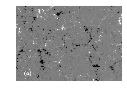
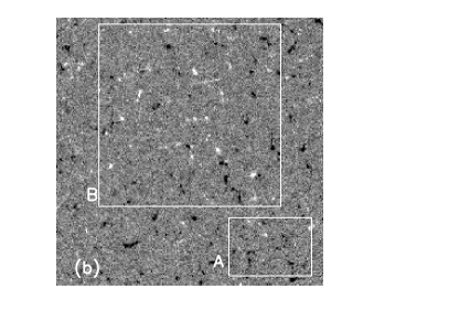
Figure 1.: Magnetograms of a section of quiet Sun from 19 Sept. 2008, (scaled between $\pm 100$ G). (a) From the MDI NFI instrument. (b) From SOHO/MDI in full-disk mode. Outlines show the field of view of (a) and of the $300^{\prime\prime}\times 300^{\prime\prime}$ images used below.

Potential fields are extrapolated from lower boundaries composed of the NFI magnetogram (Figure 1a) and sub-field A of the MDI magnetogram. This region is near enough to disk center that no compensation is made for surface curvature — the line-of-sight field is used as the vertical field, $B_{z}(x,y,0)$. The extrapolation yields field components on Cartesian grid points. The algorithm of Haynes & Parnell (2007) identifies each point at which tri-linear interpolation of the gridded field vectors vanish: magnetic null points.

The heights of null-points directly found this way can be summarized as a density, $\rho_{N}(z)$, shown as the solid curves in Figure 2a. The null column, $N_{z}(z)$, shown in Figure 2b is the number of null points, per surface area, above a given height. For the surface area of the entire magnetogram (the right axis) the number of nulls above $z\simeq 8$ Mm falls to only a handful, and the cumulative density suffers from statistical errors.

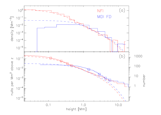
Figure 2.: The density of null points above the Hinode magnetogram (red) and sub-field A of the MDI full disk magnetogram (blue). (a) The density, $\rho_{N}(z)$, of null points found on a gridded extrapolation (solid) and by spectral estimate (dashed). (b) The column density, $N_{n}(z)$ found by integrating $\rho_{N}(z)$ downward. Left axis shows the value in Mm^-2, the right axis gives the total number of null points found on the grid.

Comparison reveals that additional spatial resolution yields more null points in the potential extrapolation from an ideal photospheric surface ($z=0$), but the additional null points are, as expected, at very low altitude. Hence, the number of coronal null points ($z>1.5$ Mm) is much less dependent on resolution.

2. The Spectral Estimate

An alternative to direct identification of null points is an estimate based on the isotropized Fourier spectrum of the magnetogram, $S(k)$, developed by Longcope et al. (2003). Figure 3a shows the spectra from various magnetograms, computed out to $k_{c}=2\sqrt{\pi}/\Delta x$ in order that the the total Fourier-space area, $\pi k_{c}^{2}$, matches that occupied by the actual magnetogram with $\Delta x\times\Delta x$ pixels.

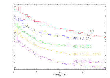
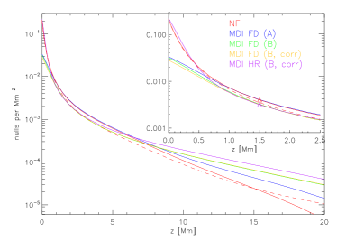
Figure 3.: (a) The isotropized spectra, $S(k)$, for different magnetograms, plotted in different shades, offset vertically for clarity. Dashed lines are $S(k)\sim e^{-2kd}$, with $d=1.2$ Mm, for comparison. (b) Spectral estimates of the null column densities using the same shades. Triangles mark the column above $z=1.5$ Mm. The dashed line is from the NFI spectrum, but with $\bar{B}_{z}=0$.

The spectral estimate of null density depends on the variance, $\sigma_{z}^{2}(z)$, of the vertical component of the extrapolated field as well as on an inverse characteristic length scale, $q(z)$, defined by a related integral

$$\sigma_{z}^{2}(z)=2\pi\int_{0}^{\infty}S(k)e^{-2kz}\,k\,dk~{}~{},~{}~{}q^{2}(z)={2\pi\over\sigma_{z}^{2}(z)}\int_{0}^{\infty}S(k)e^{-2kz}\,k^{3}\,dk~{}~{}.$$ (1)

Longcope et al. (2003) showed that under the assumption that $B_{z}(x,y,0)$ was a homogeneous, Gaussian random field, the density of magnetic null points is

$$\rho_{N}(z)~{}=~{}G(\bar{B}_{z}/\sigma_{z})\,q^{3}(z)~{}~{},$$ (2)

where $G(\zeta)$ is a dimensionless function (Longcope et al. 2003). The function depends on the mean vertical field strength $\bar{B}_{z}$ and also weakly on another moment of the spectrum. The spectral estimate, Equation (2), is plotted in Figure 2a, as a dashed curve for each of the two magnetograms. Integrating $\rho_{N}(z)$ downward from infinity gives the column densities, $N_{n}(z)$, plotted as dashed curves in Figure 2b. In the case of NFI it appears that the spectral estimate is reasonably accurate over heights with more than a handful of null points above.

The spectral estimate depends on the isotropized spectra primarily through integrals in Equation (1). Different patches of the quiet Sun, such as regions A and B of Figure 1, have very similar spectra, as shown in Figure 3a. Larger fields, such as B, sample $S({\bf k})$ more densely and thus yield more accurate spectra. Higher resolution, on the other hand allows spectra to extend to much higher wave numbers, as does the NFI curve in Figure 3a. The spectra from instruments of all resolution and fields-of-view agree relatively well over the lowest wave numbers, $k\leq 1$ rad/Mm.

The moderate wave numbers of the MDI spectra are affected by white noise and the modulation transfer function of the imaging system, including an intentional defocusing in full-disk mode (Scherrer et al. 1995). Correcting for these effects (Longcope & Parnell 2008) yields spectra even closer to those of NFI. The NFI magnetogram is corrected by deconvolution with a PSF calculated from the lunar transit of July 2008; this has a small but noticeable effect in the data.

Using each of the spectra from Figure 3a in the spectral estimate leads to column densities shown in Figure 3b. The fact that all of these agree over $z\geq 700$ km follows from the exponential factor in Equations (1). Due to this factor the spectral estimate at a height $z$ will depend on the spectral range $k<1/z$, where all spectra are similar. The fine-scale structure contributing to the high wavenumbers in both the Hinode NFI and the high-resolution MDI spectra create a layer of null points close to the photosphere ($z<500$ km). Departures over $z>10$ Mm are due to differences in $k<0.1$ rad/Mm, where the different fields of view lead to different spectral forms.

Evaluating the columns just above the chromosphere, at $z=1.5$ Mm, gives $N_{n}(1.5\,{\rm Mm})=3.9\times 10^{-3}\,{\rm Mm}^{-2}$ for NFI and $N_{n}(1.5\,{\rm Mm})=3.1\times 10^{-3}\,{\rm Mm}^{-2}$ for MDI in high resolution (triangles in the inset). The latter is almost exactly the value found in a sample of 562 MDI quiet Sun magnetograms over 1996–1998 and 2006–2007 (Longcope & Parnell 2008). Both the NFI and MDI full-disk estimates from field A are greater over the range $1<z<2$ Mm (expanded in the inset) primarily due to the mean field over the small field of view, A: $\bar{B}_{z}\simeq-2.5$ G. The larger field of view (B) is much more flux-balanced ($\bar{B}_{z}\simeq-0.28$ G). Using the NFI spectrum with $\bar{B}_{z}=0$ in Equation (2) gives the estimates from the dashed line, falling much closer to those from field B.

Acknowledgments.

This work was supported by LWS TR&T.

References

- Cirtain et al. (2007) Cirtain, J. W., et al. 2007, Science, 318, 1580
- Craig & McClymont (1993) Craig, I. J. D., & McClymont, A. N. 1993, Astrophys. J, 405, 207
- Hassam (1992) Hassam, A. B. 1992, Astrophys. J, 399, 159
- Haynes & Parnell (2007) Haynes, A. L., & Parnell, C. E. 2007, Phys. Plasmas, 14, 2107
- Longcope et al. (2003) Longcope, D. W., Brown, D. S., & Priest, E. R. 2003, Phys. Plasmas, 10, 3321
- Longcope & Parnell (2008) Longcope, D. W., & Parnell, C. E. 2008, Solar Phys., DOI 10.1007/s11207-008-9281-x
- Scherrer et al. (1995) Scherrer, P. H., et al. 1995, Solar Phys., 162, 129
- Schrijver & Title (2002) Schrijver, C. J., & Title, A. M. 2002, Solar Phys., 207, 223
- Shibata et al. (1992) Shibata, K., et al. 1992, Proc. Astron. Soc. Japan, 44, L173