Spacetimes characterized by their scalar curvature invariants
Abstract
In this paper we determine the class of four-dimensional Lorentzian manifolds that can be completely characterized by the scalar polynomial curvature invariants constructed from the Riemann tensor and its covariant derivatives. We introduce the notion of an -non-degenerate spacetime metric, which implies that the spacetime metric is locally determined by its curvature invariants. By determining an appropriate set of projection operators from the Riemann tensor and its covariant derivatives, we are able to prove a number of results (both in the algebraically general and in algebraically special cases) of when a spacetime metric is -non-degenerate. This enables us to prove our main theorem that a spacetime metric is either -non-degenerate or a Kundt metric. Therefore, a metric that is not characterized by its curvature invariants must be of Kundt form. We then discuss the inverse question of what properties of the underlying spacetime can be determined from a given a set of scalar polynomial invariants, and some partial results are presented. We also discuss the notions of strong and weak non-degeneracy.
1 Introduction
In matters related to relativity and gravitational physics we are often interested in comparing various spacetime metrics. Often identical metrics (which, of course, would give identical physics) are given in different coordinates and will therefore be disguising their true equivalence. It is therefore of import to have an invariant way to distingush spacetime metrics. The perhaps easiest way of distinguishing metrics is to calculate (some of) their scalar polynomial curvature invariants due to the fact that inequivalent invariants implies inequivalent metrics. However, if their scalar polynomial invariants are the same, what conclusion can we draw about the (in)equivalence of the metrics? For example, if all such invariants are zero, can we say that the metric is flat? The answer to this question is known to be no, because all so-called VSI metrics have vanishing scalar invariants. Here, we will address the more general question: if two spacetimes have identical scalar polynomical curvature invariants, what can we say about these spacetimes? In particular, when do the invariants characterise the spacetime metric?
For a spacetime with a set of scalar polynomial curvature invariants, there are two conceivable ways in which the metric can be altered such that the invariants remain the same. First, the metric can be continuously deformed in such a way that the invariants remain unchanged. This is what happens for the Kundt metrics for which we have free functions which do not affect the curvature invariants. Alternatively, a discrete transformation of the metric can leave the invariants the same. A simple example of when a discrete transformation can give another metric with the same set of invariants is the pair of metrics:
| (1) | |||||
| (2) |
One can straight-forwardly check that these metrics have identical invariants but are not diffeomorphic (over the reals). These discrete transformations are more difficult to deal with but the issue will be taken up in a later section.
Therefore, first we will consider the continuous metric deformations defined as follows.
Definition 1.1.
For a spacetime , a (one-parameter) metric deformation, , , is a family of smooth metrics on such that
-
1.
is continuous in ,
-
2.
; and
-
3.
for , is not diffeomorphic to .
For any given spacetime we define the set of all scalar polynomial curvature invariants
Therefore, we can consider the set of invariants as a function of the metric and its derivatives. However, we are interested in to what extent, or under what circumstances, this function has an inverse.
Definition 1.2.
Consider a spacetime with a set of invariants . Then, if there does not exist a metric deformation of having the same set of invariants as , then we will call the set of invariants non-degenerate. Furthermore, the spacetime metric , will be called -non-degenerate.
This implies that for a metric which is -non-degenerate the invariants characterize the spacetime uniquely, at least locally, in the space of (Lorentzian) metrics. This means that these metrics are characterized by their curvature invariants and therefore we can distinguish such metrics using their invariants. Since scalar curvature invariants are manifestly diffeomorphism-invariant we can thereby avoid the difficult issue whether a diffeomorphism exists connecting two spacetimes.
2 Main Theorems
Let us first state our main theorems which will be proven in the later sections. The theorems apply to four-dimensional (4D) Lorentzian manifolds. Such spacetimes are characterized algebraically by their Petrov [1, 2] and Segre [3, 2] types or, equivalently, in terms of their Ricci, Weyl (and Riemann) types [4, 5, 6]. The notation, which essentially follows that of the cited references, is briefly summarized in Appendix A. The proofs of these theorems, which are investigated on a case by case basis in terms of the algebraic type of the curvature tensors, are long and tedious and have therefore been placed in later sections. Once all of the various cases have been explored the theorems follow.
Furthermore, let us remark on the technical assumptions made in this paper. The following theorems hold on neighborhoods where the Riemann, Weyl and Segre types do not change. In the algebraically special cases we also need to assume that the algebraic type of the higher-derivative curvature tensors also do not change, up to the appropriate order. Most crucial is the definition of the curvature operators (see later) and in order for these to be well defined, the algebraic properties of the curvature tensors need to remain the same over a neighborhood.111Alternatively, we can assume that the spacetime is real analytic. Henceforth, we will therefore assume that we consider an open neighborhood where the algebraic properties of the curvature tensors do not change, up to the appropriate order ().
The first theorem deals with the algebraic classification of the curvature tensors, and the relation to the -non-degenerate metrics.
Theorem 2.1 (Algebraically general).
If a spacetime metric is of Ricci type , Weyl type , or Riemann type , the metric is -non-degenerate.
This theorem indicates that the general metric is -non-degenerate and thus the metric is determined by its curvature invariants (at least locally, in the sense explained above). In the above, by Riemann type , we are referring to the existence of a frame in which components of boost weight +2 vanish for Riemann type , and in type there does not exist a frame in which components with boost weight +2 or -2 vanish, in this case the Weyl and Ricci canonical frames are not aligned. For the algebraically special spacetimes, we need to consider covariant derivatives of the Riemann tensor.
Theorem 2.2 (Algebraically special).
If the spacetime metric is algebraically special, but , , , or is of type or more general, the metric is -non-degenerate.
In terms of the boost weight decomposition, an algebraically special metric has a Riemann tensor with zero positive boost weight components. In general, type refers to the vanishing of boost weight components +2 and higher (but not boost weight +1 components). For example, we often use the notation , to denote a of type (but ). The above theorem indicates that if by taking covariant derivatives of the Riemann tensor you acquire positive boost weight components, then the metric is -non-degenerate. The remaining metrics which do not acquire a positive boost weight component when taking covariant derivatives, have a very special structure of their curvature tensors. Indeed, such metrics must be very special metrics:
Theorem 2.3.
Consider a spacetime metric. Then either,
-
1.
the metric is -non-degenerate; or,
-
2.
the metric is contained in the Kundt class.
This is a striking result because it tells us that metrics not determined by their curvature invariants must be of Kundt form. These Kundt metrics therefore correspond to degenerate metrics in the sense that many such spacetimes can have identical invariants. The Kundt class is defined by those metrics admitting a null vector that is geodesic, expansion-free, shear-free and twist-free (corresponding to the vanishing of the spin-coefficients , and ; see also Appendix A)
| (3) |
Any metric in the Kundt class can be written in the following canonical form [7, 4]:
| (4) |
For spacetimes with constant curvature invariants (CSI) Theorem 2.3 has an important consequence. For CSI metrics, -non-degenerate implies that the spacetime is curvature homogeneous to all orders; hence, an important corollary is a proof of the CSI-Kundt conjecture [7]:
Corollary 2.4 (CSI spacetimes).
Consider a 4-dimensional spacetime having all constant curvature invariants (CSI). Then either,
-
1.
the spacetime is locally homogeneous; or,
-
2.
a subclass of the Kundt spacetimes.
These theorems imply that the Kundt spacetimes play a pivotal role in the question of which metrics are -non-degenerate. Indeed, the Kundt metrics are the only metrics not determined by their curvature invariants (in the sense explained above).
In fact, we can be somewhat more precise since only a subclass of the Kundt spacetimes have these exceptional properties. In the analysis (described below) it is found that a Kundt metric is -non-degenerate if the metric functions in the canonical (kinematic) Kundt null frame are non-linear in (i.e., ). Hence the exceptional spacetimes are the aligned algebraically special type--Kundt spacetimes or, in short (and consistent with the terminology of the above theorem) degenerate Kundt spacetimes, in which there exists a common null frame in which the geodesic, expansion-free, shear-free and twist-free null vector is also the null vector in which all positive boost weight terms of the Riemann tensor are zero (i.e., the kinematic Kundt frame and the Riemann type aligned null frame are aligned). We note that the important Kundt-CSI and vanishing scalar invariant (VSI) spacetimes are degenerate Kundt spacetimes [8, 9, 10, 7].
3 Curvature operators and curvature projectors
In order to prove the main theorems we need to introduce some mathematical tools. These tools, although they are very simple, are extremely useful and powerful in proving these theorems.
A curvature operator, , is a tensor considered as a (pointwise) linear operator
for some vector space , constructed from the Riemann tensor, its covariant derivatives, and the curvature invariants.
The archetypical example of a curvature operator is obtained by raising one index of the Ricci tensor. The Ricci operator is consequently a mapping of the tangent space into itself:
Another example of a curvature operator is the Weyl tensor, considered as an operator, ), mapping bivectors onto bivectors.
For a curvature operator, , consider an eigenvector with eigenvalue ; i.e., . If and is the dimension of the spacetime, then the eigenvalues of are invariant. Since the Lorentz transformations, , will act via a representation on , the eigenvalues of a curvature operator is an -invariant curvature scalar. Therefore, curvature operators naturally provide us with a set of curvature invariants (not necessarily polynomial invariants) corresponding to the set of distinct eigenvalues: . Furthermore, the set of eigenvalues are uniquely determined by the polynomial invariants of via its characteristic equation. The characteristic equation, when solved, gives us the set of eigenvalues, and hence these are consequently determined by the invariants. 222 Note that the ’corresponding eigenvalues’ of the operators constructed from the covariant derivatives of the Riemann tensor are also related to scalar curvature invariants built from covariant derivatives.
We can now define a number of associated curvature operators. For example, for an eigenvector so that , we can construct the annihilator operator:
Considering the Jordan block form of , the eigenvalue corresponds to a set of Jordan blocks. These blocks are of the form:
There might be several such blocks corresponding to an eigenvalue ; however, they are all such that is nilpotent and hence there exists an such that annihilates the whole vector space associated to the eigenvalue .
This implies that we can define a set of operators with eigenvalues or by considering the products
where (as long as for all ). Furthermore, we can now define
where is a curvature projector. The set of all such curvature projectors obeys:
| (5) |
We can use these curvature projectors to decompose the operator :
| (6) |
The operator therefore contains all the information not encapsulated in the eigenvalues . From the Jordan form we can see that is nilpotent; i.e., there exists an such that . In particular, if , then is a negative/positive boost weight operator which can be used to lower/raise the boost weight of a tensor.
Considering the Ricci operator, or the Weyl operator, we can show that (where the type refers to either Ricci type or Weyl type):
-
•
Type I: , .
-
•
Type D: , .
-
•
Type II: , .
-
•
Type III: , .
-
•
Type N: , .
-
•
Type O: , .
Consider a curvature projector . Then, for a Lorentzian spacetime there are 4 categories:
-
1.
Timelike: For all , .
-
2.
Null: For all , .
-
3.
Spacelike: For all , .
-
4.
None of the above.
In the following, we shall consider a complete set of curvature projectors: . These projectors can be of any of the aforementioned categories and we are going to use the Segre-like notation to characterize the set with a comma separating time and space. For example, means we have 4 projectors: one timelike, and three spacelike. A bracket indicates that the image of the projectors are of dimension 2 or higher; e.g., means that we have two spacelike operators, and one with a 2 dimensional image. If there is a null projector, we automatically have a second null projector. Given an NP frame , then a null-projector can typically be:
Note that , but it is not symmetric. Therefore, acting from the left and right gives two different operators. Indeed, defining
we get a second null-projector being orthogonal to . The existence of null-projectors enables us to pick out certain null directions; however, note that the null-operators, with respect to the aforementioned Newman-Penrose (NP) frame, are of boost weight 0 and so cannot be used to lower/raise the boost weights. In particular, considering the combination we see that the existence of null-projectors implies the existence of projectors of type .
The existence of curvature projectors is important due to the following result:
Theorem 3.1.
Consider a spacetime metric and assume that there exist curvature projectors of type , or . Then the spacetime is -non-degenerate.
Proof.
Consider first the case . For any given curvature tensor, , we can construct the curvature tensor
This enables us to consider the curvature invariant which is, up to a constant factor, the square of the component . This implies that it is determined by the invariant (up to a sign) and we get that the spacetime is -non-degenerate.
Consider now the case . We note that in this case we cannot isolate all components of the curvature tensors. However, we can uniquely define tensors , by contractions with . The curvature invariants will now be -invariant polynomials in the components of . Hence, since is compact, the polynomials will separate the orbits. Hence, by a similar proof as in [11] we get that the spacetime is -non-degenerate.
Lastly, consider the case . In this case we can define tensors , by contractions with . The curvature invariants will be -invariant which is again compact. Hence, using a similar argument as in [11] we get that the spacetime is -non-degenerate. ∎
4 Riemann type
Let us consider first the case where the Riemann tensor is of type I or . This corresponds to the three cases: Ricci type , Weyl (Petrov) type , and Ricci and Weyl canonical frames not aligned. We shall consider these in turn.
4.1 Ricci type
This case consists of the following Segre types: , , , .
4.1.1 Segre type :
Here the eigenvalues of the Ricci operator are all distinct and we can diagonalize the Ricci operator:
It now follows from Theorem 3.1 that the spacetime is -non-degenerate.
Indeed, to determine the spacetime it is sufficient to consider . Choosing an orthonormal frame, , aligned with the eigendirections of :
where are the connection coefficients, we find that all connection coefficients must be determined by the curvature invariants.
4.1.2 Segre type :
This is the special case of above where we have . Using Theorem 3.1 the spacetime is -non-degenerate.
4.1.3 Segre type :
Here we have and from Theorem 3.1 we have that the spacetime is -non-degenerate.
4.1.4 Segre type and :
In this case, the Ricci operator has two complex conjugate eigenvalues. We can always find an orthonormal frame , so that the Ricci operator takes the form
We can now consider the complex transformation mapping the basis vectors and onto the eigenvectors and :
| (7) |
with inverse
| (8) |
We note that , , and so the set can be considered as an orthonormal frame. In this frame the Ricci operator becomes diagonal:
Therefore, we have a set of curvature projectors of the form or and we can use Theorem 3.1. The only difference is that the invariants associated to the complex frame can now be complex; however, the result still stands. Using the inverse transformation, which induces a transformation between the invariants from the complex frame to the real frame, we obtain the curvature components of the real frame. Therefore we can conclude that the spacetime is -non-degenerate.
4.2 Weyl type (Petrov type )
For the Weyl tensor any non-trivial isotropy would make it algebraically special. The isotropy group of the Weyl tensor is the subgroup of the Lorentz group whose action on the Weyl tensor leaves it invariant; for example a Petrov type D Weyl tensor has a boost-spin isotropy group. So for the Weyl tensor to be of type requires that the isotropy group is trivial. We therefore expect that we will be able to determine a unique frame using the curvature invariants.
We use the bivector formalism and write the Weyl tensor, , as an operator in 6-dimensional bivector space, . Using the following index convention:
a type I Weyl tensor can always be put into the following canonical form [3]:
| (9) |
where and not all of the , are zero.
First we note that the eigenvalues of are . As explained above, and are uniquely determined by the zeroth order Weyl invariants. The eigenbivectors are . We can therefore construct annihilator operators, , and projection operators as before (the only difference is that is 6-dimensional). The eigenbivectors correspond to (complex) antisymmetric tensors. For example, consider the eigenbivector with eigenvalue :
Hence, from this we can construct an operator
| (10) |
For the other eigenbivectors we then get (analogously):
Thus the linear set span all diagonal matrices; in particular, we can construct the projection operators:
It is clear that we will get 3 operators, , as long as the 3 sets of complex eigenvalues, , are all different. Since , this can only fail when:
The first of these is actually Weyl type , while the latter is Weyl type ; hence, these are excluded by assumption.
Therefore, we can conclude that as long as the Weyl type is (and not simpler), we can define 4 projection operators of type . Therefore, from Theorem 3.1, the spacetime is -non-degenerate.
At this stage we wish to remark on a certain subtlety in the choice of eigenvectors. From the Weyl tensor we can actually only determine the product . Therefore, we can only construct the “square” . So in order to get the operator there is an ambiguity in the choice of sign. Regarding the question of -non-degeneracy as defined above this has no consequence; however, it may have an effect on discrete changes to the metric. This sign ambiguity results in a permutation of the axes; essentially, we don’t know which axis corresponds to time. We will get back to this issue later but note that this phenomenon will recur in several cases below.
4.3 Ricci and Weyl canonical frames not aligned
Consider now the case where both the Ricci tensor and the Weyl tensor are algebraically special but where there does not exist a null-frame such that both the Ricci tensor and the Weyl tensor has only non-positive boost weights.
First, assume the Weyl type is and choose the Weyl canonical frame. For Weyl type the Weyl operator is of the form of eq. (9) with . This immediately implies we have projection operators of type .
In the Weyl canonical frame, the Ricci tensor must have both positive and negative boost weight components (or else there would exist a frame where they are aligned). Now, by symmetry, we can consider three cases for the Ricci tensor (see Appendix A for notation):
-
1.
, : Here, we use the -projection operator and we get a reduced Ricci operator of the form (in the frame):
(11) This gives two distinct eigenvalues , and hence, two additional projection operators. This case therefore reduces to the case or presented earlier. This spacetime is therefore -non-degenerate.
-
2.
, , : For this case we note that the square necessarily has boost weight +2 components. Therefore, using either or , where is a parameter, we can use the results of the previous paragraph. This case is consequently -non-degenerate.
-
3.
, , : Here we consider which necessarily has non-zero boost weight and components. This case is therefore also -non-degenerate.
Assume now Weyl type and choose the Weyl canonical frame such that . In this frame, either or is non-zero. If is zero, we replace the Ricci tensor with the square in what follows. Therefore, assume that . Consider now the operator
Under the above assumptions, this operator can be used to get projectors of type . Indeed, these projectors are aligned with the Weyl canonical frame. We can now use one of the spacelike projectors, (say), to construct the symmetric operator:
where is a parameter. We can use this operator to construct the remaining projection operators so that we have a set . This case is therefore -non-degenerate.
For Weyl type we can decompose the Weyl tensor:
where the operator is a “Weyl” operator of type while the piece is a “Weyl” operator of type . By assumption, the Ricci tensor is not aligned with the Weyl canonical frame; therefore, using the above results, this case is also -non-degenerate.
Lastly, for Weyl type , we can consider the square which is a Weyl operator of type . The above results imply that this case is -non-degenerate.
4.3.1 Summary
Therefore, we have shown that: If a 4-dimensional spacetime is either Ricci type , Weyl type or Riemann type , then it is -non-degenerate.
5 Algebraically special cases
For the algebraically special cases the Riemann tensor itself does not give enough information to provide us with all the required projection operators. Indeed, in the algebraically special cases it is also necessary to calculate the covariant derivatives. The strategy is as follows: we will consider the two cases of Weyl type and in detail. The second Bianchi identity will not be imposed at this time because we aim to use these results on more general tensors with the same symmetries, not necessarily the Weyl tensor itself. Weyl type and will now follow from these computations and Weyl type will be treated last.
We should also point out that for any symmetric tensor we can always construct a Weyl-like tensor with the same symmetries as the Weyl tensor. If is the trace-free Ricci tensor, the corresponding Weyl-like tensor is the so-called Plebański tensor. Explicitly, given the trace-free part of , denoted , the Plebański tensor is given by
| (12) |
Therefore, to any symmetric tensor there is an associated “Plebański” tensor.
Henceforth we are going to use the NP-formalism where we introduce a null frame . (We will use the notation of [2]; also see Appendix A). In order to get the desired results we introduce the canonical frames for the various algebraic types. For the Weyl tensor, , this means that we express its components in terms of the Weyl scalars . Then using the NP-connection coefficients, we can express the covariant derivative in terms of and the connection coefficients. At this stage it is useful not to assume anything about the connection (i.e., the tensor need not be the Weyl tensor of the connection). The advantage of this is that we can utilise the full formalism of projection operators without worrying about the compatibility of the Weyl tensor and the connection. Furthermore, the results obtained here will therefore be more general than what is indicated. These expressions are then utilised to obtain the required results for the curvature tensor. Another important thing to note is that when taking covariant derivatives, some of the components have terms which are partial derivatives of , while other terms are algebraic in and . These algebraic terms are most useful simply because they give algebraic relations rather than differential ones.
5.1 Weyl (Petrov) type
We choose the canonical frame for which . From the Weyl operator we can construct projectors of type where the -projector projects onto the -plane, while the -projector projects onto the -plane. In the following let us use the indices for projections onto the plane and the indices for projections onto the plane.
Calculating we get the boost weight decomposition
The key observation is that the positive boost weight components vanish if and only if and . Therefore, the idea is to define the appropriate operators so that we can isolate the necessary components.
Consider the (projected) tensor:
This tensor has the following structure,
where
| (13) | |||||
| (14) | |||||
| (15) |
Furthermore, define the trace-free tensor , and then the tensor
This tensor can be considered as an operator mapping symmetric trace-free tensors onto symmetric trace-free tensors. For simplicity, let us also consider the trace-free part of so that
Consider the trace-free tensor . The operator has eigenvalues . Therefore, as long as both and are non-zero, there are three distinct eigenvalues. Assuming , is an eigentensor if and . In this case we can consider the curvature projectors (up to scaling), . The eigentensor can again be considered as an operator mapping vectors onto vectors. The eigenvalues of are ; hence, this reduces to the case of two complex eigenvalues.
We note that if and only if . Furthermore, if either of or is non-zero we can assume, by using the discrete symmetry defined later by eq. (26), that . Therefore, (so that also) implies that the spacetime is -non-degenerate.
Therefore, assume and consider the symmetric tensor
The trace-free part of this tensor is
If , then this tensor is of type . So from the Ricci type analysis, this would imply that the spacetime is -non-degenerate.
Let us next consider the non-aligned case where , and . We can now consider the mixed tensor:
This tensor is of type I if and consequently, the spacetime is -non-degenerate.
Assume now that , , for which we still have an unused discrete symmetry (eq.(26)). If we can therefore assume that . This spacetime is thus Kundt.
Lastly, consider the case when , . This automatically implies that the spacetime is Kundt.
Let us also consider the differential which in general (not assuming the Bianchi identities are satisfied) also contributes to . We note that the Weyl invariant , for a Weyl type tensor, is given by . Therefore, we can consider the curvature tensor defined by the gradient . We can now use the -projector and project this gradient onto the -plane: .
-
1.
If is either time-like or space-like (and consequently ), we can construct another curvature projector (by considering the operator ) so that we have a set . Therefore, this case is -non-degenerate.
-
2.
If is null or zero, then either or . If then and does not contribute to positive boost weight components. Assume therefore that , which implies that . If , we can use the discrete symmetry eq.(26) so that .
If any of , or is non-zero, then is non-zero. Hence, by contracting with , we can straight-forwardly construct another projection operator so that we get a set . Therefore, this case is -non-degenerate.
5.1.1 Summary Weyl type :
A Weyl type spacetime is either -non-degenerate or Kundt. Moreover, for a Weyl type spacetime, if is of type or more general, then it is -non-degenerate.
5.2 Weyl (Petrov) type
The Weyl type tensor can be decomposed as
By using the annihilator operators and the projection operators we can, up to scaling, isolate each term in this decomposition. Each term can thus be considered a curvature operator in its own right.
In particular, by considering only the curvature tensor , this tensor is identical to a Weyl type tensor. We can therefore use these results. In addition to these results we do have an additional boost weight -2 operator . This breaks the discrete symmetry present in the Weyl type tensor and therefore restricts the choice even more. However, with minor modifications we obtain: a Weyl type spacetime is either -non-degenerate or Kundt.
We also note that for a Weyl type spacetime, the Weyl invariant as for type . Therefore, using a similar argument, a Weyl type spacetime, if is of type or more general, then it is -non-degenerate.
5.3 Weyl (Petrov) type
For the Weyl type case we get no non-trivial curvature operators from the Weyl tensor itself. The first non-trivial projection operators appears at first covariant derivative; however, in order to delineate this case completely we need to consider second covariant derivatives.
We note that for the type Weyl operator, and is of type . The proof for this case is therefore contained in the Weyl type case considered below.
5.4 Weyl (Petrov) type
Consider first the tensor
whose boost weight 0 components are of the form (it has no positive boost weight components)
Therefore, if , we can construct curvature operators of type . The curvature operator gives rise to a “Plebański” tensor of type . Therefore, by considering second covariant derivatives, it follows from the Weyl type analysis that if , the spacetime is -non-degenerate.
Henceforth, assume that (and therefore we have no projectors from first derivatives). Consider , which has the same symmetries as the Weyl tensor itself. This tensor has no positive boost weight components. Considering the boost weight 0 components, we note that is of type if and only if . Therefore, if we can use the Weyl type analysis, and calculate ; hence, this spacetime is -non-degenerate.
Therefore, consider the case where either or are zero. Define
To get a projection operator we note that the boost weight 0 components of (it has no positive boost weight components) is of the form
Therefore, if either or are non-zero, we can use this operator and we get (at least) two curvature projectors and of type . This means that we can construct a Weyl-like tensor of type . Hence, we can use the type results. Therefore, by considering third derivatives of the curvature tensors, if or is non-zero, then the spacetime is -non-degenerate.
The remaining case, for which , is a Kundt spacetime.
5.4.1 Summary Weyl type or :
Therefore, we can conclude that a Weyl type or spacetime is either -non-degenerate or Kundt.
5.5 Algebraically special Ricci type
Using the trace-free Ricci tensor, we can construct the Plebański tensor, which is a Weyl-like tensor. The corresponding algebraic classification of the Plebański tensor is called the Plebański-Petrov (PP) classification. For the various algebraically special PP types we have the following Segre types:
-
•
PP type : ,
-
•
PP type : , , , ,
-
•
PP type :
-
•
PP type : ,
-
•
PP type : , , , .
Now, since the Plebański tensor is a tensor with the same symmetries as the Weyl tensor, we can use the previous results for the PP types , , and . There is consequently only the Weyl (Petrov) type and PP type case left to consider.
5.6 Weyl type , PP-type
Let us consider the remaining Segre types assuming Weyl (Petrov) type and PP type .
5.6.1 Segre type
Using the Bianchi identities we get several differential constraints on the spin coefficients. For this Segre type we have that , so the Bianchi identities immediately imply . In addition, we get the following restrictions:
Furthermore, after some manipulation of the remaining Bianchi identities, we get
and
We now split the analysis into 3 cases, according to whether is timelike, spacelike or null.
If is timelike, we immediately have that this spacetime is -non-degenerate since we can use as a timelike operator, and hence we obtain operators of type .
If is spacelike, we can always use the remaining freedom to choose . This implies that . Furthermore, which means we have an additional spacelike projection operator. Therefore, we have a set , which can be used to give a “PP-type” D tensor. Hence, using second covariant derivatives, we find that this is either Kundt or -non-degenerate.
Lastly, is null. If is zero, from the Bianchi identities we find that this is a symmetric space, and hence, is actually locally homogeneous (and Kundt). If is null, we consider . If this is non-zero we get an additional projection operator and thus a set . This would therefore give a “PP-type” D and hence, by considering second derivatives, this is either Kundt or -non-degenerate. Therefore, let us assume . The Bianchi identities now imply that . Using the symmetric operator we get that this is either of types , or . The first two of these give a type “Plebański” tensor which means, by considering second derivatives, they are either -non-degenerate or Kundt. For the last case, , we can combine with the Ricci operator to break the symmetry down to type which gives a “Plebański” of type . Therefore, by considering third and fourth derivatives, we get that this is -non-degenerate or Kundt. 333Note that this is the only case in which we have needed to utilize fourth derivatives; it is possible, by explicitly calculating the components of , that we need only consider third derivatives, but we have not done this here.
5.6.2 Segre type
This is actually Ricci type and is therefore -non-degenerate.
5.6.3 Segre type
Choosing a frame where is a constant we get, after using the Bianchi identities (and some manipulation), . We then calculate the second derivatives and compute the operator , which gives operators of type , assuming . This again gives “PP-type” D tensor and hence, by calculating third derivatives, this is -non-degenerate or Kundt.
5.6.4 Segre type
This is the maximally symmetric case and is therefore Kundt.
In addition to Weyl-type , Ricci-type or Riemann-type , we have shown that there are -non-degenerate metrics with algebraically special curvature types and further conditions on the spin-coefficients. These are summarized in Tables (1) and (2).
| P-type | Conditions |
|---|---|
| I | — |
| D or II | |
| N or III |
| Segre type of | Conditions |
|---|---|
| — | |
| const., (3rd deriv.) | |
6 Curvature invariants
We have addressed the question of what is the class of Lorentzian manifolds that can be completely characterized by the scalar polynomial invariants constructed from the Riemann tensor and its covariant derivatives. Let us now consider the ’inverse’ question: given a set of scalar polynomial invariants, what can we say about the underlying spacetime? In practice, it is somewhat tedious and a lengthy ordeal to determine the spacetime from the set of invariants. However, in most circumstances we only need some partial results or we are dealing with special cases. Let us discuss how to determine, from the invariants, whether the spacetime is -non-degenerate.
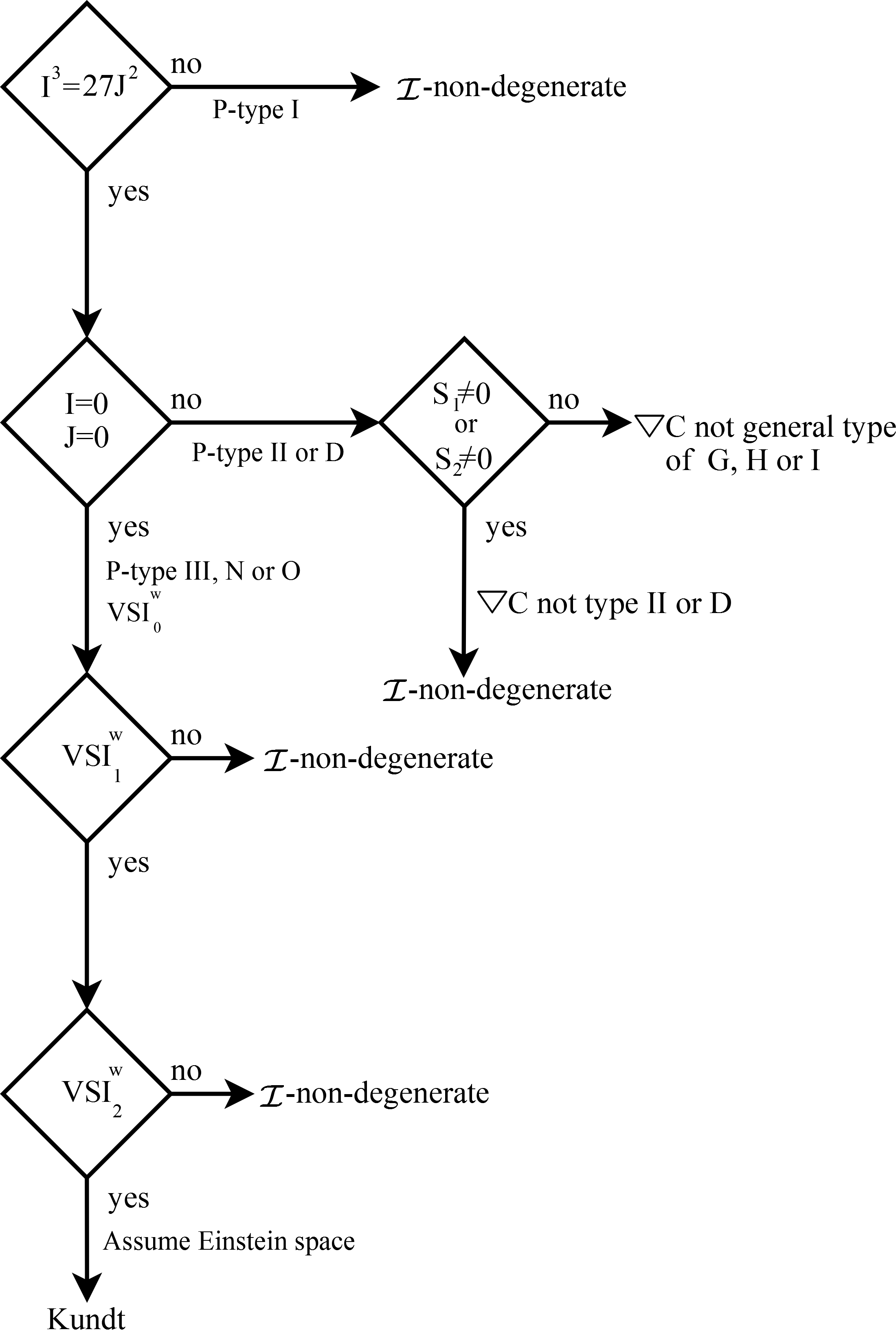
We remind the reader that the zeroth order Weyl invariants are and , and if all Weyl invariants up to order vanish, we will denote this by VSI.
Proposition 6.1.
If , then the spacetime is -non-degenerate.
This follows easily from the fact that if then the spacetime is of Weyl (Petrov) type I.
If (Weyl type or D), we need to go to higher order invariants in order to check whether it is -non-degenerate or not. Ideally, we would like to have a set of syzygies which gives the appropriate condition for this to be the case. Such a complete set is not known. However, we have found two such syzygies which gives a sufficient condition for -non-degeneracy. A number of invariants of were constructed with degrees ranging from 2 to 4 (see Appendix C for details). Imposing the minimal number of conditions required for the normal form of a -type (boost weight +3,+2,+1 vanish) or D (only boost weight 0 is nonzero) results in a degree 8 syzygy, , and a degree 16 syzygy, , amongst our invariants. Therefore if or then is not of type or . Next, we showed that using the normal form of a -type (all components nonzero) or (boost weight +3 vanish) or (boost weight +3, +2 vanish) then and . It is important to note that this implication refers only to the general types of , and and there is no consideration of a secondary alignment type or any further algebraic specialization within these types. Indeed, it is possible that there is an algebraically special subcase, for example of a -type I, that results in . A stronger statement relating invariants of to its algebraic type may be achieved by considering a different basis of invariants and a finer algebraic classification of . Initially, one would attempt to construct a set of pure invariants that was complete within each algebraic type , , and , including special subcases. We have excluded type since such a set of invariants is equivalent to type , and also types , or since these invariants vanish. By completeness of the set, an algebraic specialization would result in a dependence amongst invariants and hence syzygies arise characterizing the algebraically special type. We now have the following invariant characterizations of -non-degeneracy.
Proposition 6.2.
If , but or , then the spacetime is -non-degenerate.
The remaining cases are when both and are zero, and hence, the spacetime is VSI:
Proposition 6.3.
Assume a spacetime is VSI. Then:
-
1.
If it is not VSI, it is -non-degenerate.
-
2.
If it is VSI, but not VSI, it is -non-degenerate.
To prove the final result below, we shall assume for simplicity that the spacetime is Einstein, so that . We therefore only have to consider the Ricci scalar () and the Weyl invariants. If this is not the case, then we would need to include the Ricci and mixed invariants. This can be done in a straight-forward manner. A summary of these results is given in Figure 1.
Proposition 6.4.
Assume a spacetime is Einstein. Then:
3. If it is VSI, then it is Kundt.
From the above results we have conditions on the scalar invariants (in terms of the Weyl tensor and its covariant derivatives) to determine whether the spacetime is -non-degenerate. Consequently, we have a number of conditions in terms of scalar invariants that can be used to determine when a spacetime is not -non-degenerate and hence an aligned algebraically special type- (or degenerate) Kundt spacetime.
Let us further consider to what extent the class of degenerate Kundt spacetimes can be characterized by their scalar curvature invariants. Clearly such spacetimes are algebraically special and of type (or more special) and hence . If , then if the spacetime is of Weyl type , then if and only if from the results in [8] (the definitions of the invariants and are given therein). Similar results follow for Weyl type spacetimes (in terms of the invariants and ) and in the conformally flat (but non-vacuum) case (in terms of similar invariants and constructed from the Ricci tensor) [8]. If (Weyl types and ): essentially if , we can construct positive boost weight terms in the derivatives of the curvature and determine an appropriate set of scalar curvature invariants. For example, consider the positive boost weight terms of the first covariant derivative of the Riemann tensor, . If the spacetime is -non-degenerate, then each component of is related to a scalar curvature invariant. In this case, in principle we can solve (for the positive boost weight components of ) to uniquely determine in terms of scalar invariants, and we can therefore find necessary conditions for the spacetime to be degenerate Kundt (there are two cases to consider, corresponding to whether is zero or non-zero). We note that even if the invariants exist in principle, it may not be possible to construct them in practice.
7 Weakly and Strongly -non-degenerate
Until now we have only considered -non-degeneracy in terms of a local deformation of the metric. It is also of interest to know whether a -non-degenerate metric is unique under a discrete transformation. We shall call a spacetime such that the set of invariants uniquely specifies the metric strongly -non-degenerate. Similarly, we shall call a spacetime such that the set of invariants only defines a unique metric up to discrete transformations weakly -non-degenerate.
Let us revisit the examples given by eqs. (1) and (2) in the Introduction. These two examples are both of Weyl type , but they are of Segre type and . Hence, the eigenvalues of the Ricci operator is the same but we cannot, from the invariants alone, determine which eigenvalue is associated with the timelike direction and which is associated with the spacelike direction. This is linked to the fact that the map where we swap time with a space direction is not a Lorentz transformation. Note that permuting any two axes in the Riemannian-signature case is an transformation, while permuting time and space in the Lorentzian case is not an transformation. Therefore, there is no distinction between weakly and strongly -non-degenerate in the Riemannian case.
In most cases we do actually have a frame in which we know which direction is time. However, if we are only handed a set of invariants we would not have such a frame and, a priori, we would not know which eigenvalue is associated with time. We also note that the ambiguity in choosing a projection operator in certain cases is linked to the same problem; we do not necessarily know which eigenvalue is associated with time.
Therefore, the question of which -non-degenerate metrics are strongly -non-degenerate is linked to the question of when the time direction can be uniquely specified from the set of invariants.
Consider an invariant . Then we can consider the gradient, , which is a curvature “vector”. Assume that the metric is -non-degenerate, in which case we always have a timelike projection operator, . Therefore, we can consider . Now, if then clearly it is timelike and the invariant . Therefore, we could uniquely specify time, because would give us the time direction. So if there exists an invariant for which is timelike (and non-zero), this spacetime is strongly -non-degenerate.
A similar conclusion is reached if we have three spacelike projection operators and all of these have similar non-zero gradients. To be more precise:
Proposition 7.1.
Consider a (weakly) -non-degenerate spacetime. Then, if either:
-
1.
there exists an invariant , where is a curvature 1-tensor, such that ; or,
-
2.
there exist curvature 1-tensors , and such that the invariants , , , and
then the spacetime is strongly -non-degenerate.
Proof.
In case (1) we can construct a timelike projection operator, and the result follows. In case (2) there exist three spacelike projection operators, and the condition that ensures that these are linearly independent. Hence, the timelike vector is orthogonal to these three and the result follows. ∎
Therefore, the only spacetimes that are weakly -non-degenerate but not strongly -non-degenerate must have a timelike and a spacelike derivative which annihilate all invariants. If the spacetime is weakly -non-degenerate, but not strongly -non-degenerate, there must consequently exist a timelike vector, , and a spacelike vector, , for which
for all scalar invariants . If , it also follows that . Therefore, there will be a set of vectors, , closed under commutation (consequently, the Jacobi identity will also be satisfied), which annihilates all curvature invariants. This has several consequences. First, this set will span a timelike (sub)manifold of dimension 2, 3 or 4. We can therefore locally introduce normal coordinates, so that the invariants only depend on the normal coordinates; i.e., (dim 2), (dim 3) or (dim 4, and the spacetime is a CSI spacetime). Second, by the assumption that this spacetime is weakly -non-degenerate, and the fact that these invariants only depend on the coordinates , there exists an orthonormal frame such that all components of the curvature tensors only depend on the normal coordinates [12, 2].
This indicates that these vectors that annihilate all invariants have a special geometric meaning. First, let us consider an arbitrary curvature tensor of rank , , being a sum, tensor products and contractions of the Riemann tensor and its covariant derivatives. Since this tensor has as many covariant as contravariant indices, we can interpret this as a curvature operator, , mapping rank contravariant tensors into rank contravariant tensors. Let us denote as the tensor algebra of all such curvature operators. It is clear that all polynomial curvature invariants can be considered as complete contractions of operators in .
Theorem 7.2.
Consider a spacetime which is (weakly) -non-degenerate, and a vector field . Then the following conditions are locally equivalent:
-
1.
for all curvature invariants .
-
2.
The Lie derivative of any curvature operator with respect to , vanishes; i.e.,
Proof.
(1) (2): Assume that for all curvature invariants . Consider the 1-parameter group of diffeomorphisms, , associated with the vector field . Then
Assuming the conditions hold over a neighborhood , this can be integrated and we get, at a point , . Hence, along the integral curves the value of the invariants do not change. Consider now the Lie derivative of an arbitrary curvature operator (e.g., see [12]):
where is the -transformed tensor defined by:
The action of preserves the form and symmetries of a tensor. Thus the transformed tensor will be a curvature tensor of the same kind as . The curvature invariants at will be for and for . From the above, these invariants are the same and, from the assumption of -non-degeneracy, the invariants characterise the spacetime, which means that there exists a frame such that the components of the curvature tensors do not change along . This frame essentially is the eigenvalue frame of the curvature tensors. In particular, the projection operators define this frame.
If is an eigenvector of , then
where hatted quantities are transformed under . Eigenvectors are therefore transformed onto eigenvectors of . Using the fact that there exists a frame so that , means that the components remain the same in this frame. For a symmetric operator the eigenvectors are orthogonal and we can introduce a basis of orthonormal eigenvectors with duals . Consider now a symmetric projection operator, , written in the eigenvector basis:
where the indices run over a subset of eigenvectors with the same eigenvalue, and the hatted basis is the transformed basis. From the above discussion we see that the eigenspaces are -invariant, and hence there is a transformation matrix such that , and . Consequently,
and the curvature projection operators are -invariant. Therefore, since all can be expanded in terms of these projection operators and the curvature invariants (since it is -non-degenerate), we have that and (2) follows.
(2) (1): This follows trivially from the observation that and the properties of the Lie derivative. ∎
Corollary 7.3.
If there exists a non-zero vector field, , fulfilling
for all curvature operators , then the spacetime possesses a Killing vector field, .
Proof.
This follows from the equivalence principle [2]. The Cartan scalars are related to the components of the Riemann tensor and its derivatives, and along the integral curves of we can use at any given point . We want to compare the tensors at and . Consider an arbitrary even-ranked curvature tensor . By raising or lowering indices appropriately, we get an operator . Since the Lie derivative of along vanishes, there is a frame such that and has identical components. Therefore, by raising and lowering the indices appropriately, the components of and are also the same. The Cartan invariants of and are therefore the same. For a curvature tensor, , of odd rank we consider , which is of even rank, and use the fact that is continuous in . Therefore, there exists a frame such that all the components of any curvature tensor are identical at and . The equivalence principle now implies that , for any given , is an isometry; hence, there must exist a Killing vector field which generates an isometry such that . ∎
Note that in most cases and are the same. However, in some very special cases with additional symmetries they need not be (although locally they are of the same causality; e.g., they are both timelike or both spacelike). For example, for flat space the curvature vanishes identically; hence, for all and any curvature tensor , although not all are Killing vectors. However, in these special cases there will always exist at least two Killing vectors.
Therefore, to conclude:
Corollary 7.4.
If a spacetime is weakly -non-degenerate but not strongly -non-degenerate, then it possesses locally (at least) one timelike Killing vector and one spacelike Killing vector.
8 Conclusions
In this paper we have addressed the question of what is the class of Lorentzian manifolds that can be completely characterized by the scalar polynomial invariants constructed from the Riemann tensor and its covariant derivatives. In the Riemannian case the manifold is always locally characterized by the scalar polynomial invariants and, therefore, all of the Cartan invariants are related to the scalar curvature invariants [2]. We have generalized these results to the Lorentzian case.
We have introduced the important notion of -non-degenerate spacetime metrics. In order to prove the main theorems, which is done on a case-by-case (depending on the algebraic type) using a boost weight decomposition, we have introduced an appropriate set of curvature operators and curvature projectors. In the (algebraically) general case we have shown that if a 4D spacetime is either Ricci type , Weyl type or Riemann type , then it is -non-degenerate, which implies that the spacetime metric is determined by its curvature invariants (at least locally, in the sense explained above).
For the algebraically special cases the Riemann tensor itself does not give enough information to provide us with all the required projection operators, and it is also necessary to consider the covariant derivatives. In terms of the boost weight decomposition, for an algebraically special metric (which has a Riemann tensor with zero positive boost weight components) which is not Kundt, by taking covariant derivatives of the Riemann tensor positive boost weight components are acquired and a set of higher derivative projection operators are obtained. Consequently, we found that if the spacetime metric is algebraically special, but , , or is of type I or more general, the metric is -non-degenerate.
The remaining metrics which do not acquire a positive boost weight component when taking covariant derivatives have a very special curvature structure. Indeed, in our main theorem we proved that a spacetime metric is either -non-degenerate or the metric is a Kundt metric. This is very striking result because it implies that a metric that is not determined by its scalar curvature invariants must be of Kundt form. The Kundt metrics which are not -non-degenerate therefore correspond to degenerate metrics in the sense that many such metrics can have identical scalar invariants. This exceptional property of the the degenerate Kundt metrics essentially follows from the fact that they do not define a unique timelike curvature operator.
The results in the case of Petrov type I spacetimes in 4D follow from the above theorems. Although these results were not previously known, some partial results for 4D Weyl (Petrov) type I spacetimes, which are consistent with the above analysis, can be deduced from previous work. This is discussed in the next section (also see Appendix D).
Therefore, if a spacetime is -non-degenerate and the algebraic type is explicitly known (using, for example, the Plebański notion for the Segre type in which commas are used to distinguish between timelike and spacelike eigenvectors and their associated eigenvalues, as is common in general relativity), the spacetime can be completely classified in terms of its scalar curvature invariants.
There are a number of important consequences of the results obtained. A corollary of the main theorem applied to spacetimes with constant curvature invariants (CSI) is a proof of the CSI-Kundt conjecture in 4D [13]. In future work we will study CSI spacetimes in more detail [14].
We then considered the inverse question: given a set of scalar polynomial invariants, what can we say about the underlying spacetime? In 4D we can partially characterize the Petrov type in terms of scalar curvature invariants. In most circumstances we only need some partial results or necessary conditions. For example, we found that if , or if but the invariants or , then the spacetime is -non-degenerate. Some results were then presented in the remaining cases when both and are zero, and hence the spacetime is VSI.
We also discussed whether a -non-degenerate metric is unique under a discrete transformation. We introduced the notion strong and weak non-degeneracy. We provided a necessary criterion to determine spacetimes that are weakly -non-degenerate but not strongly -non-degenerate .
Having determined when a spacetime is completely characterized by its scalar curvature invariants, it is also of interest to determine the minimal set of such invariants needed for this classification. For example, in 4D there are results on determining the Riemann tensor in terms of zeroth order scalar curvature invariants (and determining a minimal set of such invariants) [15]. It is also of interest to study when a spacetime can be explicitly constructed from scalar curvature invariants.
This work is also of importance to the equivalence problem of characterizing Lorentzian spacetimes (in terms of their Cartan scalars) [2]. Clearly, by knowing which spacetimes can be characterized by their scalar curvature invariants alone, the computations of the invariants (i.e., simple polynomial scalar invariants) is much more straightforward and can be done algorithmically (i.e., the full complexity of the equivalence method is not necessary). On the other hand, the Cartan equivalence method also contains, at least in principle, the conditions under which the classification is complete (although in practice carrying out the classification for the more general spacetimes is difficult, if not impossible). Therefore, in a sense, the full machinery of the Cartan equivalence method is only necessary for the classification of the degenerate Kundt spacetimes (which we shall address in future work).
Let us briefly discuss this further in the context of two simple examples, which also serve to illustrate the results of the main theorem:
-
1.
The Schwarzschild vacuum type spacetime is an example of an -non-degenerate spacetime. In the canonical coordinate form of the metric as given in [16], the two scalar polynomial invariants and are functionally independent and can be used to solve for and , and all of the algebraically independent Cartan scalars , , , and are consequently related to the polynomial curvature invariants and [16]. In particular, , , so that and . We note that the second derivative Cartan scalars have the following boost weights: is +2, is -2 and is 0.
-
2.
A spatially homogeneous vacuum plane wave, which is a special subcase of a Petrov type vacuum spacetime admitting a covariantly constant null vector, belongs to the class of vanishing scalar invariant (VSI) spacetimes [8] and is consequently an example of a degenerate Kundt spacetime. Since it is a VSI spacetime, all scalar polynomial invariants are zero. However, distinct VSI spacetimes give rise to a distinct set of Cartan scalars [2] (e.g., in flat space all of the Cartan scalars are zero). A spatially homogeneous vacuum plane wave has two non-trivial Cartan scalars, and .
9 Discussion
We have addressed the question of what is the class of Lorentzian manifolds that can be completely characterized by the scalar polynomial invariants constructed from the Riemann tensor and its covariant derivatives. In particular, we proved the result that this is true in the case of Petrov type I spacetimes in 4D. This result was not previously known. However, some partial results for 4D Weyl (Petrov) type I spacetimes are known, which are consistent with the above analysis. Let us review these results.
Essentially, in the case of Petrov (Weyl) type I, there exists a unique frame so that all components of the Riemann tensor are related to curvature invariants. Indeed, in general there are four different curvature invariants (e.g., corresponding to the complex invariants and ), so that all invariants (which depend on coordinates) are functionally dependent on these four invariants. Problems arise in degenerate cases and cases with symmetries. It is also known that all Petrov type I spacetimes are completely backsolvable [15].
Let us consider the Petrov type I case in more detail. From [17, 3] (also see Appendix D) it follows that if a 4D spacetime is of Petrov type I it can be classified according to its rank and it is either:
-
1.
curvature class A (and the holonomy group is general and of type ),
-
2.
curvature class C (and of holonomy type or , with restricted Segre type).
Now, suppose the components of the Riemann tensor are given in a coordinate domain with metric . In case (1), where the curvature class is of type A, for any other metric with the same components it follows that (where is a constant); i.e., the metric is determined up to a constant conformal factor and the connection is uniquely determined. This implies that all higher order covariant derivatives of the Riemann tensor are completely determined; i.e., given , all of the components of the covariant derivatives are determined and we only need classify the Riemann tensor itself. (Note that all of the scalar polynomial curvature invariants are then determined, at least up to an overall constant factor).
We can then pass to the frame formalism and determine the frame components of the Riemann tensor (to do this we need the metric to determine the orthogonality of the frame vectors and hence construct the frame; since is specified up to an overall constant conformal factor, orthogonality is unique). The Petrov type I case is completely backsolvable [15] and hence the frame components are completely determined by the zeroth order scalar invariants. Therefore, it follows that the spacetime is completely characterized by its scalar curvature invariants in this case.
Let us now consider case (2), where the curvature class is . Again, let us suppose that the are given in with metric . If is any other metric with the same , it follows that
(where and are constants). The equation
| (17) |
has a unique non-trivial solution for . Note that implies that and hence , where is the Euler density:
If , then and the metric is determined up to a constant conformal factor (and the holonomy type is ). This is similar to the first case discussed above, but now some information on the covariant derivative of the Riemann tensor is necessary (to ensure ). Hence, first order curvature invariants are needed for the classification of the spacetime. Since implies that , where
it follows that the invariant implies that in this case.
If , then , and since eqn. (17) has a unique solution, is recurrent. If is null, the spacetime is algebraically special, and since we assume that the Petrov type is I, this is not possible. Hence, is (a) timelike (TL) or (b) spacelike (SL) and is, in fact, covariant constant (CC).
In case (2a), the spacetime admits a TL CC vector field . The holonomy is , with a TL holonomy invariant subspace which is non-degenerately reducible, and is consequently locally decomposable (and static). There exist local coordinates (with ) such that the metric is given by
| (18) |
where is independent of . The metric is unique up to an overall constant scaling and a time translation , where (reflecting the non-uniqueness of the TL CC vector up to a constant scaling ). All of the non-trivial components of the Riemann tensor and its covariant derivatives are constructed from the 3D positive definite metric , and can be classified by the corresponding 3D Riemann curvature invariants. In this case (and case () there is an ignorable coordinate and all invariants are functions of independent functions; must be used to uniquely fix the frame, and hence we need information from the first order scalar invariants.
In case (2b), the spacetime admits a SL CC vector field . The holonomy is , there exists a holonomy invariant vector which is non-degenerately reducible, and is this locally decomposable. Choosing local coordinates in which the SL CC vector , the metric is given by
| (19) |
and is independent of . The metric is unique up to an overall constant conformal factor and a space translation . Classification now reduces to the classification of the class of 3D Lorentzian spacetimes with Lorentzian metric (the subclass such that (2) is of Petrov type ). We can now iterate the procedure for 3D Lorentzian spacetimes (such that (2) is Petrov type ). In the degenerate cases in which additional KV are admitted, we will be led to the locally homogeneous case, and hence the 4D Petrov type I locally homogeneous spacetimes (which are characterized by their constant scalar invariants). Indeed, in 3D the Riemann tensor is completely determined by the Ricci tensor. There always exists a frame in which the components of the Ricci tensor are constants [7] and so in this case the 4D spacetime is Petrov type and (curvature homogeneous [18]), and hence generically locally homogeneous.
Acknowledgments
We would like to thank Robert Milson for useful comments and questions on our manuscript, and to Lode Wylleman for pointing out a mistake. This work was supported by the Natural Sciences and Engineering Research Council of Canada.
Appendix A Notation
Throughout we have used a Newman-Penrose (NP) tetrad given by with inner product
| (20) |
and directional derivatives defined by
| (21) |
Associated with an NP tetrad are the following definitions for the connection coefficients that appear frequently above
| (22) |
with the remaining ones being similarly defined. Given the frame components , we have the definitions for the Weyl scalars
and the Ricci scalars
| (23) |
Given a covariant tensor with respect to an NP tetrad (or null frame), the effect of a boost , allows to be decomposed according to its boost weight
| (24) |
where denotes the boost weight components of . An algebraic classification of tensors has been developed [6, 5] which is based on the existence of certain normal forms of (24) through successive application of null rotations and spin-boost. In the special case where is the Weyl tensor in four dimensions, this classification reduces to the well-known Petrov classification. However, the boost weight decomposition can be used in the classification of any tensor in arbitrary dimensions. As an application, a Riemann tensor of type has the following decomposition
| (25) |
in every null frame. A Riemann tensor is algebraically special if there exists a frame in which certain boost weight components can be transformed to zero, these are summarized in Table 3.
A useful discrete symmetry is the following (orientation-preserving) Lorentz transformation:
| (26) |
which interchanges the boost weights, , and makes the replacements
| (27) |
| Riemann type | Conditions |
|---|---|
| G | — |
| I | |
| II | |
| III | |
| N | |
| D | |
| O | all vanish (Minkowski space) |
Appendix B Some special operators
Consider the case where we have a tensor , where
This tensor can be considered as an operator:
where is the vector space of symmetric 2-tensors .
Therefore, we can consider the eigentensors of this map in the standard manner. We can construct a set of projectors projecting onto each corresponding eigenspace. Assume that is of rank 1 (as an operator). If is the corresponding (normalized) eigenvector, this means that
We can now consider the eigenvectors of . We are actually not considering the operator itself, but rather . However, can also be considered as an operator:
Assume that and are eigenvectors of with eigenvalues and , respectively. Then, if ,
and is therefore an eigenvector of with eigenvalue . Clearly, has the same eigenvalue as , so we will not be able to distinguish these using projection operators. Furthermore, if , then has the same eigenvalue as .
The above construction is useful in several cases. An example that recurs is the case where has two one-dimensional eigenspaces spanned by and , say. Assume also that . Then, has two projection operators:
| (28) | |||||
| (29) |
We see that this is somewhat unfortunate because in spite of the fact that sees the difference between the vectors and , does not. This is related to the fact that for some spacetimes there exists a discrete symmetry which interchanges two spacetimes with identical curvature invariants. Here this manifests itself in that we cannot actually determine which eigenvector correspond to which eigenvalue.
Appendix C Algebraically special
The relationship between the invariants of the Weyl tensor and the Petrov type is well known; however, this is not the case for the covariant derivative of the Weyl tensor. A similar analysis for would require an algebraic classification based on its boost weight decomposition, and a complete set of its first order invariants. We do not attempt to solve this general problem but rather provide some relations relevant to our paper. Restricting attention to four dimensions we define the following tensors
| (30) | |||||
| (31) | |||||
| (32) | |||||
| (33) |
where the number above the tensor refers to the degree in or . All of these tensors are constructed purely from with the exception of (which involves ). Next, we consider the following first order invariants
| (34) | |||||
| (35) | |||||
| (36) | |||||
| (37) | |||||
| (38) |
in which denotes the invariant of degree in or . Since the aligned frames of and need not be the same, the are mixed invariants and the remaining invariants are pure invariants. For and algebraically general (type ) we obtain the following syzygies
which are the result of identities, symmetries and dimensionally dependent relations444Thanks to Jose M. Martin-Garcia for pointing this out to us. [19]. In subsequent calculations we always impose these syzygies so that our set reduces to ten invariants. Now consider of algebraically special type, which is obtained by setting the minimal number of appropriate boost weight components to vanish. We obtain the following results:
-
1.
If is type or (i.e., boost weight
components vanish) then the syzygies and hold.
-
2.
If is type or type (i.e., boost weight vanish), or type (i.e., boost weight vanish) then, in general, and .
The second statement refers to the most general types of , or where no further algebraically special subcases are taken into account. Below are the expressions for and . Note that is linear in , and when , we use this syzygy in the derivation555 does not appear in . of ; hence these two invariant expressions are generally independent. In type or we can regard as expressing the dependency of in terms of the other invariants of . In each of the appear quadratically whereas each of appear quartically therefore one of these invariants is dependent with respect to the other invariants in . Since these syzygies are of degree 8 and 16, and the invariants considered here are of maximum degree 4, one would expect and to attain a simpler form if expressed in terms of higher degree invariants. These calculations were performed with the aid of GRTensorII [20].
Appendix D Curvature
Let be a 4-dimensional smooth connected Hausdorff manifold admitting a global smooth Lorentz metric with associated curvature tensor . It will be convenient to describe a simple algebraic classification of according to its rank (relative to ). This classification is easily described geometrically and is a pointwise classification [3].
A skew-symmetric tensor of type or at is called a bivector. If is such a bivector, the rank of any of its (component) matrices is either two or four. In the former case, one may write (e.g. in the case) for (or alternatively, ) and is called simple, with the 2-dimensional subspace (2-space) of spanned by referred to as the blade of . In the latter case, is called non-simple.
The metric converts into a Lorentz inner product space and thus it makes sense to refer to vectors in and covectors in the cotangent space to at (using to give a unique isomorphism , that is, to raise and lower tensor indices) as being timelike, spacelike, null or orthogonal, using the signature . The same applies to 1-dimensional subspaces (directions) and 2- and 3-dimensional subspaces of or . A simple bivector at is then called timelike (respectively, spacelike or null) if its blade at is a timelike (respectively a spacelike or null) 2-space at . A non-simple bivector at may be shown to uniquely determine an orthogonal pair of 2-spaces at , one spacelike and one timelike, and which are referred to as the canonical pair of blades of . A tetrad of members of is called a null tetrad at if the only non-vanishing inner products between its members at are . Thus and are null.
D.1 Classification
Define a linear map from the 6-dimensional vector space of type bivectors at into the vector space of type tensors at by . The condition (2) shows that if a tensor is in the range of then
| (39) |
and so can be regarded as a member of the matrix representation of the Lie algebra of the pseudo-orthogonal (Lorentz) group of . Using one can divide the curvature tensor into five classes.
- Class
-
This is the most general curvature class and the curvature will be said to be of (curvature) class at if it is not in any of the classes , , or below.
- Class
-
The curvature tensor is said to be of (curvature) class at if the range of is 2-dimensional and consists of all linear combinations of type tensors and where and with a null tetrad at . The curvature tensor at can then be written as
(40) where , .
- Class
-
The curvature tensor is said to be of (curvature) class at if the range of is 2- or 3-dimensional and if there exists such that each of the type tensors in the range of contains in its kernel (i.e. each of their matrix representations satisfies ).
- Class
-
The curvature tensor is said to be of (curvature) class at if the range of is 1-dimensional. It follows that the curvature components satisfy at for some bivector at which then satisfies and is thus simple.
- Class
-
The curvature tensor is said to be of (curvature) class at if it vanishes at .
The following results are useful [3]:
-
1.
For the classes and there does not exist such that for every in the range of .
-
2.
For class , the range of has dimension at least two and if this dimension is four or more the class is necessarily .
-
3.
The vector in the definition of class is unique up to a scaling.
-
4.
For the classes and there does not exist such that , whereas this equation has exactly one independent solution for class and two for class .
-
5.
The five classes , , , and are mutually exclusive and exhaustive for the curvature tensor at . If the curvature class is the same at each then will be said to be of that class.
D.2 Properties
Suppose that the components of the Riemann tensor are given in a coordinate domain with metric . Suppose that is another metric with the same components . It follows from [17] that:
where .
Note that for some smooth 1-form on the open subset . Using condition (2) above and the Ricci identity we get , which implies ; thus and so is locally a gradient. Hence, for each , there is an open neighborhood of on which for some smooth function . Then on , satisfies . Further, if is any other local metric defined on some neighborhood of and compatible with then satisfies condition (2) on and hence, on , for some positive smooth function . From this and the result it follows that is a constant multiple of on .
References
- [1] A.Z. Petrov, Einstein spaces (Pergamon, 1969)
- [2] H. Stephani, D. Kramer, M. A. H. MacCallum, C. A. Hoenselaers, E. Herlt 2003 Exact solutions of Einstein’s field equations, second edition (Cambridge University Press; Cambridge).
- [3] G S Hall, 2004, Symmetries and curvature structure in general Relativity (World Science, Singapore).
- [4] A. Coley, 2008, Class. Quant. Grav. 25, 033001.
- [5] R. Milson, A. Coley, V. Pravda and A. Pravdova, 2005, Int. J. Geom. Meth. Mod. Phys. 2, 41.
- [6] A. Coley, R. Milson, V. Pravda and A. Pravdova, 2004, Class. Quant. Grav. 21, L35.
- [7] A. Coley, S. Hervik and N. Pelavas, 2006, Class. Quant. Grav. 23, 3053.
- [8] V. Pravda, A. Pravdová, A. Coley and R. Milson, 2002, Class. Quant. Grav. 19, 6213.
- [9] A. Coley, R. Milson, V. Pravda and A. Pravdova, 2004, Class. Quant. Grav. 21, 5519.
- [10] A. Coley, A. Fuster, S. Hervik, N. Pelavas, 2006, Class. Quant. Grav. 23, 7431
- [11] F. Prüfer, F. Tricerri and L. Vanhecke, 1996, Trans. American Math. Soc., 348, 4643.
- [12] S Kobayashi and K. Nomizu, 1963, Foundations of Differential Geometry, Volume 1 (Interscience Publishers).
- [13] A. Coley, S. Hervik and N. Pelavas, 2008, Class. Quantum Grav. 25, 025008.
- [14] A. Coley, S. Hervik and N. Pelavas, 2009, Class.Quant.Grav. 29 125011.
- [15] E. Zakhary and J. Carminati, 2001, J. Math. Phys. 42, 1474; J. Carminati, E. Zakhary, and R. G. McLenaghan, 2002, J. Math. Phys. 43, 492; J. Carminati and E. Zakhary, 2002, J. Math. Phys. 43, 4020
- [16] F. M. Paiva, M. J. Reboucas and M. A. H. MacCallum, 1993, Class. Quant. Grav. 10, 1165.
- [17] G S Hall and W Kay, 1988, J. Math. Phys. 29, 428
- [18] R. Milson and N. Pelavas, 2008, Class. Quantum Grav. 25 012001; ibid. arXiv:0711.3851 ; ibid. arXiv:gr-qc/0702152.
- [19] J. M. Martin-Garc a, D. Yllanes and R. Portugal, 2008, Comp. Phys. Commun. 179 586-590, arXiv:0802.1274 [cs.SC]
- [20] This is a package which runs within Maple. It is entirely distinct from packages distributed with Maple and must be obtained independently. The GRTensorII software and documentation is distributed freely on the World-Wide-Web from the address http://grtensor.org