Extended Hubbard model in the presence of a magnetic field

Abstract

Within the Green’s function and equations of motion formalism it is possible to exactly solve a large class of models useful for the study of strongly correlated systems. Here, we present the exact solution of the one-dimensional extended Hubbard model with on-site $U$ and first nearest neighbor repulsive $V$ interactions in the presence of an external magnetic field $h$, in the narrow band limit. At zero temperature our results establish the existence of four phases in the three-dimensional space ($U,n,h$) - $n$ is the filling - with relative phase transitions, as well as different types of charge ordering. The magnetic field may dramatically affect the behavior of thermodynamic quantities, inducing, for instance, magnetization plateaus in the magnetization curves, and a change from a single to a double-peak structure in the specific heat. According to the value of the particle density, we find one or two critical fields, marking the beginning of full or partial polarization. A detailed study of several thermodynamic quantities is also presented at finite temperature.

1 Introduction

In physics exact solutions are of great importance since, in some cases, an approximation may introduce dramatically dominating errors, resulting in an incorrect description of the phenomenon under study. Recently, within the Green’s function and equations of motion formalism, we have shown that it is possible to exactly solve a large class of models useful for the study of strongly correlated systems Mancini05_06 ; mancini2 . By exactly solvable we mean that it is always possible to find a set of eigenenergies and eigenoperators of the Hamiltonian closing the hierarchy of the equations of motion. Thus, one can obtain exact expressions for the relevant Green’s and correlation functions in terms of a finite set of parameters manciniavella .

The aim of the present paper is twofold. First, we would like to further develop our previous work on the exact solution of the one-dimensional extended Hubbard model in the atomic limit (AL-EHM) mancini2 , by extending it to a more general situation in which a finite magnetization may be induced by an external magnetic field. Secondly, the AL-EHM exhibits interesting features at low temperatures, and one of the most fascinating characteristic feature is that it shows magnetic plateaus. Interestingly, magnetization plateaus have been predicted also for spin-one bosons in optical lattices imambekov04 . By atomic limit, according to the conventional definition used in the literature, we mean the classical limit of the model, i.e., we set from the very beginning the hopping matrix elements $t_{ij}=0$. One may obtain different results by treating the problem with nonzero hopping and then taking the limit to zero.

A uniform magnetic field, introduced through a Zeeman term, has dramatic effects both on the $T=0$ phase diagram and on the behavior of several thermodynamic quantities. We study the properties of the system as functions of the external parameters $n$, $T/V$, $U/V$ and $h/V$ (throughout the paper we set $V=1$ as the unit of energy), allowing for the on-site interaction $U$ to be both repulsive and attractive. In fact, the parameter $U$ can represent the effective interaction coupling taking into account also other interactions. Owing to the particle-hole symmetry, it is sufficient to explore the interval $[0,1]$ for the parameter $n$. The chemical potential is self-consistently determined as a function of the external parameters. We address the problem of determining the zero-temperature phase diagram in the ($U$, $n$, $h$) space and we find various phase transitions (PTs), as well as magnetization plateaus. At $T=0$, for attractive on-site interactions, the magnetic field does not play any role if its intensity is $h<|U|/2$: the ground state is a collection of doublons (sites with two electrons of opposite spin), and there are no neighbor sites occupied. The magnetic energy is not strong enough to break the doublons. On the other hand, for strong repulsive on-site interactions, it is sufficient a small nonzero value of the magnetic field to have a finite magnetization. In the intermediate regions, the competition among $U$, $V$ and $h$ determines the phase structure.

Relevant thermodynamic quantities, such as the double occupancy, the charge and spin susceptibilities, the specific heat and the entropy are systematically computed both at $T=0$ and as functions of the temperature. For all values of the particle density, one finds a critical value (dramatically depending on $U$ and $n$) of the magnetic field $h_{s}$ above which the ground state is ferromagnetic. In this state, every occupied site contains one and only one electron, aligned along the direction of $h$. For strong repulsive on-site interactions, one finds $h_{s}=0$, i.e., the spin are polarized as soon as the magnetic field is turned on. Furthermore, for attractive on-site interactions and $0.5<n\leq 1$, one observes the existence of two critical fields, namely: $h_{c}$, up to which no magnetization is observed, and $h_{s}$, marking the beginning of full polarization. This is analogous to the finite field behavior of the $S=1$ Haldane chain haldane .

The addition of a homogeneous magnetic field does not dramatically modify the framework of calculation given in Ref. mancini2 , provided one takes into account the breakdown of the spin rotational invariance. For the sake of comprehensiveness, in Section 2, we briefly report the analysis leading to the algebra closure and to analytical expressions of the retarded Green’s functions (GFs) and correlation functions (CFs). The GFs and CFs depend on a set of internal parameters, which can be determined by means of algebra constraints Mancini05_06 ; manciniavella , allowing us to provide an exact and complete solution of the one-dimensional AL-EHM in the presence of a magnetic field. In Section 3 we analyze the properties of the system at zero temperature. We characterize the different phases emerging in the phase diagram drawn in the ($U,n,h$) space, by studying the behavior of the chemical potential and of various local properties (double occupancy, short-range correlation function, magnetization); Section 4 is devoted to the study of the finite temperature properties. Further to the study of the quantities analyzed in Section 3, we also present results for the charge and spin susceptibilities, the specific heat and the entropy. Finally, Sec. 5 is devoted to our conclusions and final remarks, while the Appendix reports some relevant computational details.

2 The model

The one-dimensional extended Hubbard model in the presence of an external homogeneous magnetic field is described by the following Hamiltonian

$$\begin{split}H&=\sum_{ij}[t_{ij}-\delta_{ij}\mu]c^{\dagger}(i)c(j)+U\sum_{i}{n_{\uparrow}(i)n_{\downarrow}(i)}\\ &+\frac{1}{2}\sum_{i\neq j}{V_{ij}n(i)n(j)}-h\sum_{i}n_{3}(i).\end{split}$$ (1)

$n(i)=c^{\dagger}(i)c(i)$ is the charge density operator, $c(i)$ $(c^{\dagger}(i))$ is the electron annihilation (creation) operator - in the spinor notation - satisfying canonical anti-commutation relations. $n_{3}(i)$ is the third component of the spin density operator, also called the electronic Zeeman term,

$$n_{3}(i)=n_{\uparrow}(i)-n_{\downarrow}(i)=c_{\uparrow}^{\dagger}(i)c_{\uparrow}(i)-c_{\downarrow}^{\dagger}(i)c_{\downarrow}(i).$$ (2)

Here we do not consider the orbital interaction with the magnetic field and we use the Heisenberg picture: $i=({\bf i},t)$, where i stands for the lattice vector ${\bf R}_{i}$. The Bravais lattice is a linear chain of $N$ sites with lattice constant $a$. $\mu$ is the chemical potential; $h$ is the intensity of the external magnetic field and $U$ and $V$ are the strengths of the local and intersite interactions, respectively. In the atomic limit, if one considers only first neighboring sites interactions, the Hamiltonian (1) takes the form

$$H=\sum_{i}\left[-\mu n(i)+U{D(i)}+\frac{1}{2}Vn(i)n^{\alpha}-hn_{3}(i)\right],$$ (3)

where $D(i)$ is the double occupancy operator, defined as $D(i)=n_{\uparrow}(i)n_{\downarrow}(i)=n(i)[n(i)-1]/2$. Hereafter, for a generic operator $\Phi(i)$, we define $\Phi^{\alpha}(i,t)=\sum_{j}\alpha_{ij}\Phi(j,t)$, where $\alpha_{ij}$ is the projection operator over first nearest neighboring sites.

2.1 Composite fields and equations of motion

By taking time derivatives of increasing order of the fermionic field $c(i)$, the dynamics generates other field operators of higher complexity (composite operators). However, the number of composite operators is finite because of the recurrence relation

$$[n^{\alpha}(i)]^{k}=\sum_{m=1}^{4}A_{m}^{(k)}[n^{\alpha}(i)]^{m},$$ (4)

which allows one to write the higher-power expressions of the operator $n^{\alpha}(i)$ in terms of the first four powers. The coefficients $A_{m}^{(k)}$ are rational numbers satisfying the relations $\sum_{m=1}^{4}A_{m}^{(k)}=1$ and $A_{m}^{(k)}=\delta_{m,k}$ ($k=1,\ldots,4$), explicitly given in Ref. mancini05b . As a result, a complete set of eigenoperators of the Hamiltonian (3) can be found.

Upon introducing the Hubbard operators $\xi(i)=[n(i)-1]c(i)$ and $\eta(i)=n(i)c(i)$, one may define the composite field operator

$$\psi(i)=\begin{pmatrix}\psi^{(\xi)}(i)\\ \psi^{(\eta)}(i)\end{pmatrix}=\begin{pmatrix}\psi_{\uparrow}^{(\xi)}(i)\\ \psi_{\downarrow}^{(\xi)}(i)\\ \psi_{\uparrow}^{(\eta)}(i)\\ \psi_{\downarrow}^{(\eta)}(i)\end{pmatrix},$$ (5)

where

$$\psi_{\sigma}^{(\xi)}(i)=\begin{pmatrix}\xi_{\sigma}(i)\\ \xi_{\sigma}(i)[n^{\alpha}(i)]\\ \vdots\\ \xi_{\sigma}(i)[n^{\alpha}(i)]^{4}\end{pmatrix},\;\psi_{\sigma}^{(\eta)}(i)=\begin{pmatrix}\eta_{\sigma}(i)\\ \eta_{\sigma}(i)[n^{\alpha}(i)]\\ \vdots\\ \eta_{\sigma}(i)[n^{\alpha}(i)]^{4}\end{pmatrix},$$ (6)

where $\sigma=\{\uparrow,\downarrow\}$. With respect to the case of zero magnetic field mancini2 , the degrees of freedom have doubled, since one has to the take into account the two nonequivalent directions of the spin. By exploiting the algebraic properties of the operators $n(i)$ and $D(i)$, it is easy to show that the fields $\psi^{(\xi)}(i)$ and $\psi^{(\eta)}(i)$ are eigenoperators of the Hamiltonian (3) mancini05b :

$$\begin{split}i\frac{\partial}{\partial t}\psi^{(\xi)}(i)&=[\psi^{(\xi)}(i),H]=\varepsilon^{(\xi)}\psi^{(\xi)}(i),\\ i\frac{\partial}{\partial t}\psi^{(\eta)}(i)&=[\psi^{(\eta)}(i),H]=\varepsilon^{(\eta)}\psi^{(\eta)}(i).\end{split}$$ (7)

$\varepsilon^{(\xi)}$ and $\varepsilon^{(\eta)}$ are the $10\times 10$ energy matrices:

$$\varepsilon^{(\xi)}=\left({{\begin{array}[]{*{20}c}{\varepsilon_{\uparrow}^{(\xi)}}&0\\ 0&{\varepsilon_{\downarrow}^{(\xi)}}\\ \end{array}}}\right),\qquad\varepsilon^{(\eta)}=\left({{\begin{array}[]{*{20}c}{\varepsilon_{\uparrow}^{(\eta)}}&0\\ 0&{\varepsilon_{\downarrow}^{(\eta)}}\\ \end{array}}}\right),$$ (8)

where

$$\varepsilon_{\sigma}^{(\xi)}=\begin{pmatrix}-\scriptstyle\mu-\sigma h&\scriptstyle 2V&\scriptstyle 0&\scriptstyle 0&\scriptstyle 0\\ \scriptstyle 0&\scriptstyle-\mu-\sigma h&\scriptstyle 2V&\scriptstyle 0&\scriptstyle 0\\ \scriptstyle 0&\scriptstyle 0&\scriptstyle-\mu-\sigma h&\scriptstyle 2V&\scriptstyle 0\\ \scriptstyle 0&\scriptstyle 0&\scriptstyle 0&\scriptstyle-\mu-\sigma h&\scriptstyle 2V\\ \scriptstyle 0&\scriptstyle-3V&\scriptstyle\frac{25}{2}V&-\scriptstyle\frac{35}{2}V&\scriptstyle-\mu-\sigma h+10V\end{pmatrix},$$ (9)

$$\varepsilon_{\sigma}^{(\eta)}=\begin{pmatrix}\scriptstyle U-\mu-\sigma h&\scriptstyle 2V&\scriptstyle 0&\scriptstyle 0&\scriptstyle 0\\ \scriptstyle 0&\scriptstyle U-\mu-\sigma h&\scriptstyle 2V&\scriptstyle 0&\scriptstyle 0\\ \scriptstyle 0&\scriptstyle 0&\scriptstyle U-\mu-\sigma h&\scriptstyle 2V&\scriptstyle 0\\ \scriptstyle 0&\scriptstyle 0&\scriptstyle 0&\scriptstyle U-\mu-\sigma h&\scriptstyle 2V\\ \scriptstyle 0&\scriptstyle-3V&\scriptstyle\frac{25}{2}V&\scriptstyle-\frac{35}{2}V&\scriptstyle U-\mu-\sigma h+10V\end{pmatrix}.$$ (10)

The eigenvalues of the matrices $\varepsilon^{(\xi)}$ and $\varepsilon^{(\eta)}$ are

$$E^{(\xi)}=\begin{pmatrix}E_{\uparrow}^{(\xi)}\\ E_{\downarrow}^{(\xi)}\end{pmatrix},\qquad E^{(\eta)}=\begin{pmatrix}E_{\uparrow}^{(\eta)}\\ E_{\downarrow}^{(\eta)}\end{pmatrix},$$ (11)

where

$$\begin{split}E^{(\xi)}_{p,\sigma}&=-\mu-\sigma h+(p-1)V,\\ E_{p,\sigma}^{(\eta)}&=U-\mu-\sigma h+(p-1)V,\end{split}$$ (12)

with $p=1,\ldots,5$. Although at the level of equations of motion the two fields $\psi^{(\xi)}(i)$ and $\psi^{(\eta)}(i)$ are decoupled, they are indeed coupled by means of the self-consistent equations which determine the correlators appearing in the normalization matrix, as shown in Subsection 2.3.

2.2 Retarded Green’s and correlation functions

The knowledge of a complete set of eigenoperators and eigenenergies of the Hamiltonian (3) allows one to exactly determine the retarded thermal Green’s function

$$G^{(a)}(t-t^{\prime})=\theta(t-t^{\prime})\langle\{\psi^{(a)}(i,t),{\psi^{a}}^{\dagger}(i,t^{\prime})\}\rangle.$$ (13)

In the above equations, $a=\xi,\eta$ and $\langle\cdots\rangle$ denotes the quantum-statistical average over the grand canonical ensemble. By means of the field equations (7), it is easy to show that the Green’s function satisfies the equation

$$[\omega-\varepsilon^{(a)}]G^{(a)}(\omega)=I^{(a)},$$ (14)

where $I^{(a)}$ is the normalization matrix

$$I^{(a)}=\langle\{\psi^{(a)}(i,t),{\psi^{(a)}}^{\dagger}(i,t)\}\rangle,$$ (15)

whose expression in discussed in the Appendix. The solution of Eq. (14) is

$$G^{(a)}(\omega)=\sum_{p=1}^{10}\frac{\sigma^{(a,p)}}{\omega-E_{p}^{(a)}+i\delta},$$ (16)

where the spectral functions $\sigma_{\mu\nu}^{(a,p)}$ can be computed by means of the formula

$$\sigma_{\mu\nu}^{(a,p)}=\Omega_{\mu p}^{(a)}\sum_{\delta}{\Omega_{p\delta}^{(a)}}^{-1}I_{\delta\nu}^{(a)}.$$ (17)

$\Omega^{(a)}$ is the $10\times 10$ matrix whose columns are the eigenvectors of the matrix $\varepsilon^{(a)}$. Explicit expressions of the matrices $\Omega^{(\xi)}=\Omega^{(\eta)}$ are reported in the Appendix. The correlation function

$$\begin{split}C^{(a)}(t-t^{\prime})&=\langle\psi^{(a)}(i,t){\psi^{(a)}}^{\dagger}(i,t^{\prime})\rangle\\ &=\frac{1}{(2\pi)}\int_{-\infty}^{+\infty}d\omega e^{-i\omega(t-t^{\prime})}C^{(a)}(\omega)\end{split}$$ (18)

can be immediately computed from Eq. (16) by means of the spectral theorem, and one finds

$$C^{(a)}(\omega)=\pi\sum_{p=1}^{10}\left[{1+\tanh\left({\frac{\beta\omega}{2}}\right)}\right]\sigma^{(a,p)}\delta[\omega-E_{p}^{(a)}],$$ (19)

where $\beta=1/k_{B}T$. At equal time, the CF is given by

$$C^{(a)}=\langle\psi^{(a)}(i){\psi^{(a)}}^{\dagger}(i)\rangle=\frac{1}{2}\sum_{p=1}^{10}T_{p}^{(a)}\sigma^{(a,p)},$$ (20)

where $T_{p}^{(a)}=1+\tanh(E_{p}^{(a)}/2k_{B}T)$. Upon introducing the parameters

$$\begin{split}n&=\langle n(i)\rangle,\\ m&=\langle n_{3}(i)\rangle,\\ \kappa^{(p)}&=\langle[n^{\alpha}(i)]^{p}\rangle,\end{split}\qquad\begin{split}\lambda^{(p)}&=\frac{1}{2}\langle n(i)[n^{\alpha}(i)]^{p}\rangle,\\ \pi^{(p)}&=\frac{1}{2}\langle n_{3}(i)[n^{\alpha}(i)]^{p}\rangle,\end{split}$$ (21)

the elements of the normalization matrix can be written as

$$\begin{split}I_{1,p}^{(\xi)}&=\kappa^{(p-1)}-\lambda^{(p-1)}+\pi^{(p-1)},\\ I_{6,p+5}^{(\xi)}&=\kappa^{(p-1)}-\lambda^{(p-1)}-\pi^{(p-1)},\\ I_{1,p}^{(\eta)}&=\lambda^{(p-1)}-\pi^{(p-1)},\\ I_{6,p+5}^{(\eta)}&=\lambda^{(p-1)}+\pi^{(p-1)},\end{split}$$ (22)

where and $p=1,\ldots,5$. All the other matrix elements can be easily computed by means of the recurrence relation (4).

2.3 Self-consistent equations

The previous analysis shows that the complete solution of the model requires the knowledge of the following 13 parameters: $\mu$, $m$, $\kappa^{(2)},\ldots,\kappa^{(4)}$, $\lambda^{(1)},\ldots,\lambda^{(4)}$, $\pi^{(1)},\ldots,\pi^{(4)}$. These quantities may be computed by using algebra constraints and symmetry requirements Mancini05_06 ; manciniavella . By recalling the projection nature of the Hubbard operators $\xi(i)$ and $\eta(i)$, it is straightforward to verify that the following algebraic properties hold

$$\begin{split}\xi^{\dagger}(i)n(i)&=0,\\ \xi^{\dagger}(i)D(i)&=0,\end{split}\qquad\begin{split}\eta^{\dagger}(i)n(i)&=\eta^{\dagger}(i),\\ \eta^{\dagger}(i)D(i)&=0.\end{split}$$ (23)

These are fundamental relations and constitute the basis to construct a self-consistent procedure to compute the various parameters of the model. Upon splitting the Hamiltonian (3) as the sum of two terms:

$$\begin{split}H&=H_{0}+H_{I},\\ H_{I}&=2Vn(i)n^{\alpha}(i),\end{split}$$ (24)

the statistical average of any operator $O$ can be expressed as

$$\langle O\rangle=\frac{\langle Oe^{-\beta H_{I}}\rangle_{0}}{\langle e^{-\beta H_{I}}\rangle_{0}},$$ (25)

where $\langle\cdots\rangle_{0}$ stands for the trace with respect to the reduced Hamiltonian $H_{0}$: $\langle\cdots\rangle_{0}={\rm Tr}\{\cdots e^{-\beta H_{0}}\}/{\rm Tr}\{e^{-\beta H_{0}}\}$. The Hamiltonian $H_{0}$ describes a system where the original lattice has been reduced to a central site and to two unconnected sublattices. Thus, in the $H_{0}$-representation, the correlation functions connecting sites belonging to disconnected sublattices can be decoupled. Within this scheme, the unknown parameters can be written as functions of only two parameters $X_{1}=\langle n^{\alpha}(i)\rangle_{0}$ and $X_{2}=\langle D^{\alpha}(i)\rangle_{0}$, in terms of which one may find a solution of the model. By exploiting the translational invariance along the chain, one can impose $\langle n(i)\rangle=\langle n^{\alpha}(i)\rangle$ and $\langle D(i)\rangle=\langle D^{\alpha}(i)\rangle$, finding, thus, two equations allowing one to determine $X_{1}$ and $X_{2}$ as functions of $\mu$:

$$\begin{split}F_{1}(X_{1},X_{2};\mu)&=0,\\ F_{2}(X_{1},X_{2};\mu)&=0.\end{split}$$ (26)

The chemical potential $\mu$ can be determined by means of the equation

$$n=F_{3}(X_{1},X_{2};\mu).$$ (27)

The explicit expressions of the functions $F_{1}$, $F_{2}$, and $F_{3}$ are given in the Appendix. Equations (26) and (27) constitute a system of coupled equations allowing us to ascertain the three parameters $\mu$, $X_{1}$ and $X_{2}$ in terms of the external parameters of the model $n$, $h$, $U$, $V$, and $T$. Once these quantities are known, all the properties of the model can be computed.

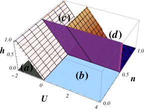
Figure 1: The phase diagram in the space $(U,n,h)$ at $T=0$ and $V=1$. The four different phases are characterized by different distributions of the particles. Phase ($a$) is characterized by zero magnetization and by only non-neighboring doubly occupied sites. In the phase ($b$) the electrons singly occupy non-neighboring sites with all the spins parallel to $h$. In the phase ($c$) one finds both singly polarized and doubly occupied non-neighboring sites, whereas in the phase ($d$) neighboring sites can be occupied but no doublons are to be found.

3 The zero-temperature phase diagram

In this Section we derive the phase diagram of the AL-EHM in the $(U,n,h)$ space. By numerically solving the set of equations (26) and (27), we study the $T=0$ behavior of relevant physical quantities. This investigation allows us to envisage the distribution of the particles along the chain, for different densities, as well as the magnetic properties of the system. The results obtained are displayed in Fig. 1: one recognizes the already known mancini2 four different phases found at $h=0$ extending in the $h$ direction.

The phase structure is determined by the three competing terms of the Hamiltonian: the repulsive intersite potential (disfavoring the occupation of neighboring sites), the magnetic field (aligning the spins along its direction, disfavoring thus double occupancy) and the on-site potential, which can be either attractive or repulsive. According to the values of these competing terms, one may distinguish the different phases, characterized by different values of the double occupancy, the chemical potential, and of the parameters defined in Eq. (21).

Phase ($a$) is observed in the region $0\leq n\leq 1$ for attractive on-site potential ($U<0$) and $h<|U|/2$; it is just a continuation along the $h$ axis of the phase observed at $h=0$ mancini2 and is characterized by a zero magnetization $m=0$. The parameters $X_{1}$ and $X_{2}$ take the values $X_{1}=2X_{2}=2n/(2-n)$. The chemical potential takes the value $U/2$ for $n<1$, whereas at $n=1$ (half filling) it jumps to the value $\mu=2V+U/2$, as required by particle-hole symmetry. The distribution of the particles in the phase ($a$) is shown in Fig. 2, where we report just one possible configuration. The attractive on-site potential favors the formation of doubly occupied sites. At the same time, the nearest-neighbor repulsion $V$ disfavors the occupation of neighboring sites. This distribution of the electrons is confirmed by the expectation values $D=n/2$ and $\lambda^{(k)}=0$. When $n<1$, there is no ordered pattern in the distribution of the particles, whereas, for $n=1$, one observes the well-known checkerboard distribution of doubly-occupied sites mancini2 ; Bari71 .

Figure 2: Distribution of the particles along the chain by varying the particle density at $T=0$, $V=1$, $U<0$ and $h<|U|/2$. White and black squares denote empty and doubly-occupied sites, respectively.

The phase ($b$) is observed only for particle densities equal or less than quarter filling ($n=0.5$), in the regions ($U>0$, $\forall h$) and ($U<0$, $h>|U|/2$). In the latter region, there is a competition between the attractive on-site potential which favors the creation of doublons and the magnetic field which favors the alignment of the electrons. When $h>|U|/2$, it is energetically convenient to singly occupy non-neighboring sites. Similarly, for $U>0$, the repulsion between electrons on the same site and on neighboring sites ($V>0$), leads to a scenario where the double occupancy, as well as the short-range correlation functions $\lambda^{(k)}$, vanishes in the limit $T\to 0$. One observes that the electrons tend to singly occupy non-neighboring sites with all the spins parallel to $h$, leading to a finite magnetization $m=n$. For particle densities less than quarter filling, there is a cost in energy to add one electron which is proportional to the intensity of the magnetic field: $\mu=-h$. At $n=0.5$, the chemical potential jumps to the value $\mu=V-h$ and a long-range order is established: one observes a checkerboard distribution of singly occupied polarized sites, as evidenced in Fig. 3. In this region one finds $X_{1}=n/(1-n)$ and $X_{2}=0$.

For particle densities greater than quarter filling, the phase diagram is richer in the plane ($U,h$): one observes three phases by varying $U$ ($h$) and keeping $h$ ($U$) fixed, as evidenced in Fig. 1. Phase ($a$) has been discussed above. The phase ($c$) is observed for $0.5<n\leq 1$ and in the regions ($0<U<2V$, $h<V-U/2$) and ($U<0$, $|U|/2<h<V+|U|/2$). The chemical potential takes the value $U+h$ for $0.5<n<1$ and $2V+U/2$ at $n=1$. In this region the intersite interaction dominates: the minimization of the energy requires the extra electrons above $n=0.5$ to occupy non-empty sites. Thus, in the thermodynamic limit, there can be singly polarized and doubly occupied sites but no neighboring sites: $\langle n(i)[n^{\alpha}(i)]^{k}\rangle=0$. By increasing $n$, the number of doubly-occupied sites increases linearly, $D=n-1/2$, while the magnetization decreases as $m=1-n$. The distribution of the particles in the region $(c)$ is drawn in Fig. 3, where we represent just one possible configuration. The ground states of the Hamiltonian are checkerboard configurations where empty sites alternate with sites occupied by either two particles or one particle with polarized spin. At half filling, one observes a checkerboard distribution of only doubly occupied sites Bari71 .

Figure 3: Distribution of the particles along the chain by varying the particle density at $T=0$ and $V=1$. For $0<n\leq 0.5$, this distribution is observed both for $\{U<0$, $h>|U|/2\}$ and $\{U>0$, $\forall h\}$. For $0.5<n\leq 1$, it corresponds to the regions $\{U<0$, $|U|/2<h<V+|U|/2\}$ and $\{0<U<2V$, $h<V-U/2\}$. White and black squares denote empty and doubly-occupied sites, respectively. The squares with the arrow denote singly occupied sites with field-aligned spins.

Also the phase ($d$) is observed for both attractive and repulsive on-site interactions. In particular, when $U>2V$ the on-site interaction dominates over the nearest-neighbor repulsion $V$. The minimization of the energy requires the electrons not to be paired and allows for the occupation of neighboring sites: $D=0$ and $\lambda^{(1)}=n-1/2$. The combined action of $U$ and $h$ predominates over $V$, leading to the same distribution in the region ($0<U<2V$, $h>V-U/2$). For $U<0$, a strong magnetic field ($h>V+|U|/2$) dominates both the on-site and intersite potentials, resulting on the absence of doublons and the possibility to have neighboring sites occupied. In this phase, one finds $X_{1}=1$ and $X_{2}=0$. For $n<1$ the energy necessary to add one electron is $\mu=2V-h$. At $n=1$ the chemical potential jumps to the value $\mu=2V+U/2$. Since in this state every occupied site contains one and only one polarized electron, the ground state is ferromagnetic and the magnetization is $m=n$, as evidenced in Fig. 4.

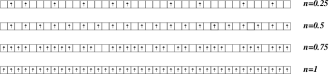
Figure 4: Distribution of the particles along the chain by varying the particle density at $T=0$ and $V=1$. This distribution is observed in two different parameters regions, namely $\{U<2V$, $h>V+U/2\}$ and $\{U>2V,\forall h\}$. White squares denote empty sites, whereas the squares with the arrow denote singly occupied sites with field-aligned spins.

These peculiar distributions of the electrons along the chain by varying the magnetic field give rise to the formation of plateaus in the magnetization curves. By increasing the magnetic field, there are plateaus whose starting points depend on the particle density, as well as on the on-site potential: one identifies two critical values of the magnetic field. The nonzero magnetization can either begin from $h=0$ or from a finite field. $h_{c}$ denotes the starting point of a nonzero magnetization, whereas $h_{s}$ denotes the value of the magnetic field when it reaches saturation. The results for the magnetization $m(h)$ are shown in Fig. 5. The values of $h_{c}$ and $h_{s}$ can be inferred from the previous analysis. Making reference to Fig. 5 for the different regions of $n$ and $U$, one has: $h_{c}=h_{s}=|U|/2$ (Fig. 5a), $h_{c}=|U|/2$ and $h_{s}=V+|U|/2$ (Fig. 5b), $h_{c}=0$ and $h_{s}=V-U/2$ (Fig. 5c), and $h_{c}=h_{s}=0$ (Fig. 5d).

The so-called metamagnetic behavior is clearly seen: at low temperatures the magnetization begins to show a typical $S$-shape which becomes more pronounced by further decreasing the temperature. At $T=0$ one, two or three plateaus ($m=0$, $m=1-n$ and $m=n$) are observed, according to the values of the external parameters.

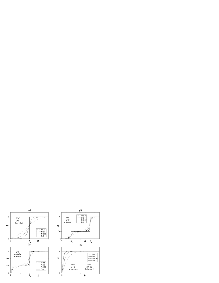
Figure 5: The magnetization $m$ as a function of the magnetic field $h$ at $V=1$ and decreasing temperatures.

These results are similar to the ones obtained in a one-dimensional spin-1 antiferromagnetic Ising chain with single-ion anisotropy chen03 ; mancini08 .

In Figs. 6 we plot the double occupancy and the chemical potential as functions of $h$ for $U=-1$, $n=0.25$, 0.75 and different temperatures. As the temperature decreases, $D$ exhibits sharp jumps, whereas $\mu$ shows discontinuity(ies). In particular: (i) for all values of the particle density, $\mu$ takes the constant value $\mu=U/2$ in the region $U<0$ and $h<|U|/2$, corresponding to $h_{s}$ ($h_{c}$) for $n=0.25$ (0.75); (ii) for $0<n<0.5$ and $h>h_{s}$, $\mu$ decreases with the law $\mu=-h$. On the other hand, for $0.5<n<1$, $\mu$ first increases with the law $\mu=U+h$ until $h_{s}=V+|U|/2$. Further increasing $h$ one observes a decrease of the chemical potential following the law $\mu=2V-h$. As it is evident from Figs. 6, at $T=0$ and for repulsive on-site interactions, the double occupancy shows a one or a two step-like behavior according to the particle density. The steps occur at the values of the magnetic field where PTs are observed.

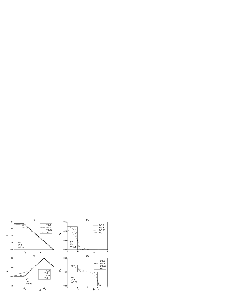
Figure 6: The chemical potential and the double occupancy at $V=1$, $U=-1$ and different values of the temperature, for $n=0.25$ and $n=0.75$.

In closing this Section, it is worthwhile to mention that at $T=0$ and $h=0$ all the phases (with the exception of the case $n=1$ and $U<2V$) exhibit a macroscopic degeneracy growing exponentially with the volume of the lattice. A nonzero magnetic field can lift the degeneracy of the ground states at quarter and half filling, even for repulsive on-site interactions.

4 Finite temperature

In this Section we shall investigate the finite temperature properties of the AL-EHM. We study the behavior of the system as a function of the parameters $n$, $T$, $U$ and $h$, and again we take $V=1$ as the unit of energy and we set the Boltzmann’s constant $k_{B}=1$.

4.1 Thermal properties

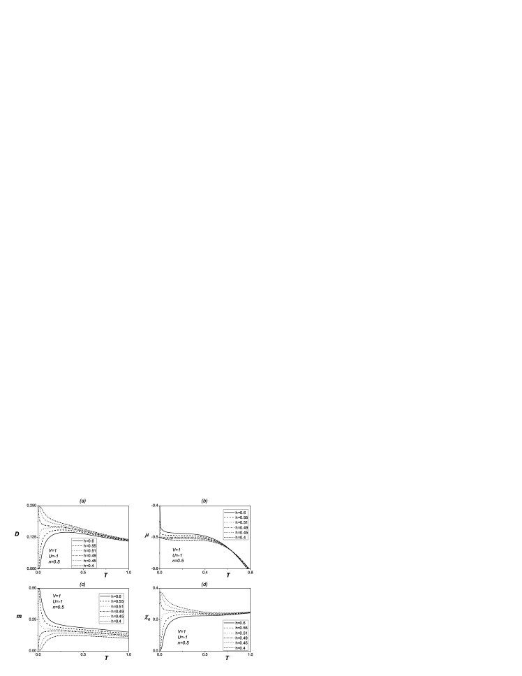
Figure 7: (a) The double occupancy, (b) the chemical potential, (c) the magnetization $m$, and (d) the charge susceptibility as functions of the temperature for $V=1$, $U=-1$ and $n=0.5$ in the neighborhood of $h_{s}=0.5$, where the transition from phase ($a$) to phase ($b$) occurs.

In Fig. 7 we show the behavior of different quantities as a function of $T$ for $n=0.5$, $U=-1$ and various values of $h$ in the vicinity of the critical point $h_{s}=|U|/2=0.5$. These behaviors are not peculiar to the given values of the parameters, but are always observed in the neighborhood of all critical values of $h$ when the system goes from one phase to another. In the high temperature regime the double occupancy, the chemical potential and the magnetization decrease by increasing $T$, whereas for $T\to 0$ they tend to two different constants, as shown in Figs. 7. At $h=h_{s}$ and $T=0$ there is a phase transition: for the considered values of the external parameters, one finds that the double occupancy jumps from zero to $n/2$, the magnetization from zero to $n$ and the chemical potential from $U/2$ to $V-h$. Also the charge susceptibility, defined as $\chi_{c}=N~{}n^{2}+k_{B}~{}T$ $\partial n/\partial\mu$, behaves differently at low temperatures according to the value of $h$. For $h<h_{s}$ the charge susceptibility increases by decreasing $T$ and tends to $\chi_{c}=n(1-n)(2-n)$ at $T=0$. For $h>h_{s}$ the charge susceptibility decreases by decreasing $T$ and tends to $\chi_{c}=n(1-n)(1-2n)$ at $T=0$. In the particular case shown in Fig. 7d, $\chi_{c}$ vanishes for $T\to 0$ when $h>h_{s}$: the system is in a charge ordered state mancini2 . The non-vanishing of the charge susceptibility in the limit $T\to 0$ corresponds to a non-ordered ground state. For $h=h_{s}$ and $T=0$ there is a phase transition and the charge susceptibility exhibits the discontinuity $\Delta\chi_{c}=n(1-n^{2})$.

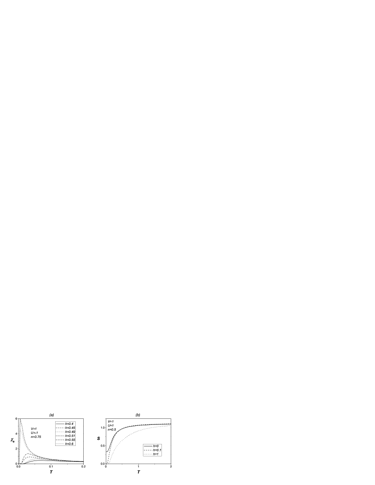
Figure 8: (a) The spin susceptibility as a function of the temperature for $V=1$, $U=-1$, $n=0.75$ in the neighborhood of $h=|U|/2$. (b) The entropy $S$ as a function of the temperature at $V=1$, $U=1$, $n=0.5$ and different values of $h$.

Another signature of the $T=0$ transition in the neighborhood of the critical values of the magnetic field is provided by the behavior of the spin susceptibility, defined as $\chi_{s}=\partial m/\partial h$. As an example, in Fig. 8a, we plot $\chi_{s}$ for $U=-1$, $n=0.75$ and different values of $h$ around $h_{c}=|U|/2$. In the high temperature regime the spin susceptibility decreases by increasing $T$. In the low temperature regimes, the spin susceptibility exhibits a peak at a temperature $T_{1}$, then decreases going to zero at $T=0$. By approaching the value $h=h_{c}$ (both from below and above) the position $T_{1}$ of the peak moves towards lower temperatures; at the same time the height $h_{1}$ of the peak increases. At $h=h_{c}$ the spin susceptibility diverges at $T=0$.

Recently, we have discuss how the entropy may be computed when the ground state is degenerate mancini2 . In this case, the zero-temperature entropy $S(0)$ is non-zero and, if the system is not confined in one of the possible phases, is not even constant but depends on the external parameters. The magnetic field can remove the $h=0$ ground state degeneracy, responsible of a finite zero-temperature entropy. This can be clearly seen in Fig. 8b where we plot the entropy as a function of the temperature at $U=1$ and $n=0.5$ for increasing values of the magnetic field. As soon as the magnetic field is turned on, the entropy vanishes in the limit $T\to 0$.

The study of the specific heat further enlightens the influence of the magnetic field on the thermodynamic behavior of the system. The specific heat is given by $C=dE/dT$, where the internal energy $E$ can be computed as the thermal average of the Hamiltonian (3) and it is given by $E=UD+2V\lambda^{(1)}-hm$. As an example of the characteristic behavior of the specific heat by varying $h$, in Fig. 9 we plot $C$ as a function of the temperature at $V=1$, $U=-1$, and $n=0.5$, for several values of the magnetic field. With the exception of the critical value $h=h_{s}$, one observes an exponential activation of $C$ with a pronounced peak, whose position depends on $h$. Furthermore, the low temperature peak observed at $n<1$ for pertinent values of the on-site potential when $h=0$, tends to disappear by approaching $h_{s}$, both from above and below. The position of the peak moves towards lower temperatures and vanishes exactly at $h=h_{s}$. Of course, also the low temperature peak with exponentially increasing height (observed at half-filling in the limit $U\to 2V$ at $h=0$ mancini2 ) survives only for small values of $h$, but disappears at $h=h_{s}$. On the other hand, for higher values of the magnetic field one always observes a double peak structure in the specific heat for all values of the particle density.

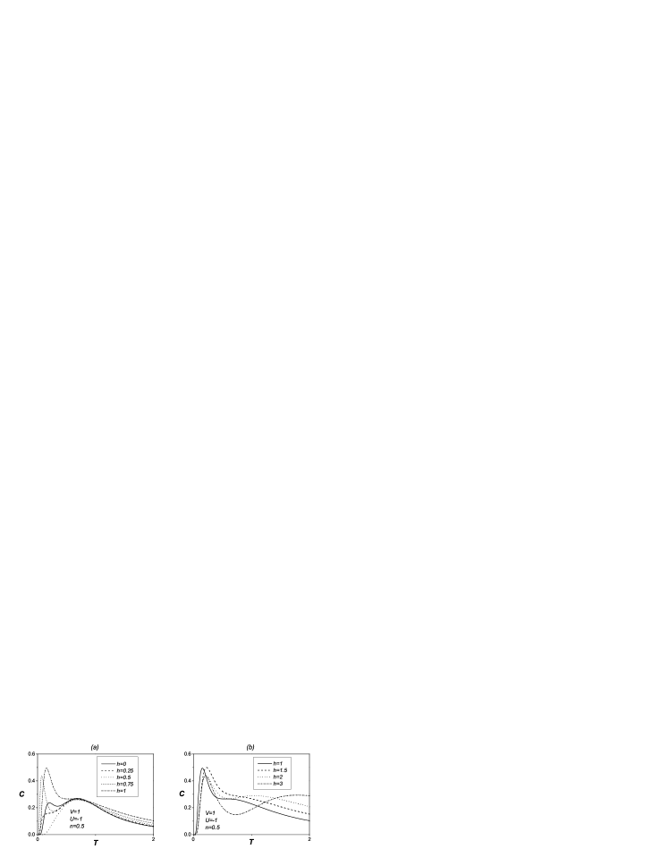
Figure 9: The specific heat $C$ as a function of the temperature for $V=1$, $U=-1$, $n=0.5$ and for different values of $h$.

In this region, the low temperature peak remains constant by varying $h$, whereas the high temperature broad peak moves towards higher temperatures by increasing $h$.

Interestingly, a change from a single to a double-peak structure by varying the magnetic field has also been observed in one-dimensional ferrimagnets with alternating spins maisinger98 .

4.2 Magnetic properties

A useful representation of the phase diagram is obtained by plotting the thermodynamic quantities as functions of the magnetic field $h$. Indeed, this representation constitutes another way to detect the zero-temperature transitions from thermodynamic data. In fact, at low temperatures, all the thermodynamic quantities that we have investigated present minima, maxima, or discontinuities in the neighborhood of the critical values of $h$ at which zero-temperature PTs occur.

As a first example, in Figs. 10a-c we plot $\chi_{c}$ as a function of the magnetic field, for $n=0.75$ and for different values of the on-site potential ($U=-1$, 1, 2.5). In the high temperature regime, the charge susceptibility is always a decreasing function of $h$. In the limit $T\to 0$, one observes two different behaviors, according to which phase the system is in: $\chi_{c}$ tends to a constant when the system is in a non-ordered phase, whereas it presents minima in correspondence of the critical values of the magnetic field, as evidenced in Fig.10.

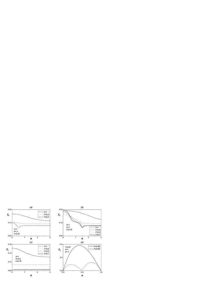
Figure 10: The charge susceptibility $\chi_{c}$ as a function of the magnetic field at different temperatures for $V=1$, $n=0.75$ and for (a) $U=-1$, (b) $U=1$, and (c) $U=2.5$. (d) $\chi_{c}$ as a function of the particle density for $V=1$, $U=-1$, $T=0.01$ and different values of $h$.

A similar behavior of the charge susceptibility is observed also for other values of the particle density. In Fig. 10d we plot $\chi_{c}$ as a function of the filling $n$ at $V=1$ and $U=-1$ and for two values of $h$ ($h=0.45$ and $h=0.55$, below and above $h_{crit}=0.5$, respectively). To simplify notation, here we shall use $h_{crit}$ to indicate either $h_{c}$ and $h_{s}$. One immediately sees that, for $T\to 0$ and $h<h_{crit}$, the charge susceptibility increases by increasing $n$ and has a maximum at quarter filling. Further increasing $n$, $\chi_{c}$ decreases and vanishes at half-filling, where, at fixed on-site potential, a zero-temperature PT occurs by varying $n$, from a non-ordered to a checkerboard distributions of doublons (see Fig. 2). When $h>h_{crit}$, at low temperatures, $\chi_{c}$ has a double peak structure with two maxima around $n=0.25$ and $n=0.75$ and two minima around $n=0.5$ and $n=1$. This implies the presence of a charge ordered state also at $n=0.5$, as evidenced by the charge distribution shown in Fig. 4.

In Figs. 11a-c we plot the spin susceptibility as a function of the magnetic field at $T=0.1$ for three representative values of $U$ ($U=-1$, $U=1$ and $U=2.1$, respectively) and for different values of the filling ($n=0.25$, 0.5, 0.75, 1). The spin susceptibility diverges in correspondence of the values $h_{crit}$ at which one moves from one magnetization plateau to the other. For low values of the magnetic field and attractive on-site interactions - corresponding to Fig. 11a - the spin susceptibility tends to vanish at low temperatures for all values of the filling: at $T=0$ all electrons are paired and no alignment of the spin is possible. By increasing $h$, the magnetic excitations break some of the doublons inducing a finite magnetization: $\chi_{s}$ has a peak, then decreases, the system having entered the successive magnetic plateau. If $0.5<n<1$ then another peak is observed, corresponding to the second jump of the magnetization when $h$ reaches the saturated value $h_{s}$. On the other hand, for repulsive on-site interactions, a very small magnetic field induces a finite magnetization (with the exception of $n=1$ when $U<2V$): $\chi_{s}$ has a maximum at $h=0$ and decreases by augmenting $h$, unless another transition line is encountered, as it happens for $0.5<n\leq 1$ and $0<U<2V$.

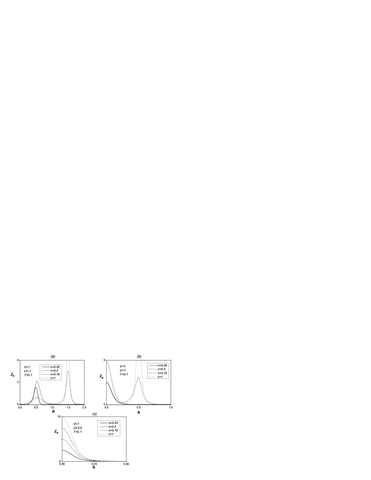
Figure 11: The spin susceptibility as a function of the magnetic field for $V=1$, $T=0.1$ and (a): $U=-1$, (b): $U=1$, (c): $U=2.5$.

In Figs. 12 we plot the entropy as a function of the magnetic field for relevant values of the particle density $n$. The entropy presents maxima in the neighborhood of the values of $h$ at which one observes zero-temperature PTs, and $S(0)$ has discontinuities right at those values. On the other hand, for sufficiently strong magnetic fields, the entropy becomes rather insensitive to variations in $h$. When $n\leq 0.5$, the entropy presents a peak around $h_{s}$ which becomes more pronounced as the temperature decreases. In the region $0.5<n<1$, at low temperatures, one finds two peaks at $h_{c}$ and $h_{s}$, respectively. Although at half filling there is a zero-temperature transition at $h_{s}$, one always finds $S(0)=0$ since the relative ground states are non-degenerate.

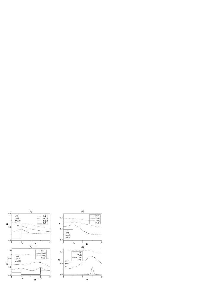
Figure 12: The entropy $S$ as a function of the magnetic field for $V=1$, $U=-1$, $T=1$, 0.5, 0.2 and (a): $n=0.25$, (b): $n=0.5$, (c): $n=0.75$, and (d): $n=1$.

5 Concluding remarks

We have evidenced how the use of the Green’s function and equations of motion formalism leads to the exact solution of the one-dimensional AL-EHM limit in the presence of an external magnetic field. We provided a systematic analysis of the model for nearest-neighbor repulsion $V$ by considering relevant thermodynamic quantities in the whole space of the parameters $n$, $T$, $h$ and $U$ (having chosen $V=1$ as the unity of energy). This study has shown that, at zero-temperature, the model exhibits phase transitions for specific values of $n$, $h$ and $U$. In particular, we have identified four phases in the ($U,n,h$) space and PTs are observed at the borders of these phases. Various types of long-range charge ordered states have been observed: (i) at half-filling for $U<2V$ and $h<V-U/2$, a checkerboard distribution of doubly-occupied sites; (ii) at quarter-filling for $U>0$, as well as for $U<0$ and $h>|U|/2$, a checkerboard distribution of polarized singly occupied sites; (iii) for $0.5\leq n\leq 1$ an ordered state with alternating empty and occupied sites in the regions ($U<0$, $|U|/2<h<V+|U|/2$) and ($0<U<2V$, $h>V-U/2$).

We derived the phase diagram in the space $(U,n,h)$ at $T=0$ by computing several quantities whose behaviors is also useful to characterize the distribution of the electrons on the sites of the chain. When plotted as functions of $h$, the chemical potential, the double occupancy as well as the magnetization, show discontinuities where PTs occur. We identified the values of the critical fields $h_{c}$ and $h_{s}$, defining, according to the value of the particle density, the beginning point of nonzero magnetization and the saturated magnetization field, respectively. Furthermore, the presence of the magnetic field may dramatically modify the behavior of several thermodynamic quantities. For instance, the charge susceptibility tends to different values in the limit $T\to 0$, depending on how strong is the magnetic field. At quarter and half filling, a strong magnetic field can also remove the macroscopic degeneracy of the ground states: as a result, the zero-temperature entropy is zero.

Appendix A Computational details

Firstly, we shall provide some more details on the matrices used in the computational framework adopted in Sec. 2. To begin with, we note that, due to the spin conservation, the normalization matrix $I^{(a)}=\langle\{\psi^{(a)}(i,t),{\psi^{(a)}}^{\dagger}(i,t)\}\rangle$ is block diagonal:

$$I^{(a)}=\left({{\begin{array}[]{*{20}c}{I^{\uparrow\uparrow,(a)}}&0\\ 0&{I^{\downarrow\downarrow,(a)}}\\ \end{array}}}\right).$$ (28)

The time translational invariance requires the $m$-matrix $m=\langle\{i\frac{\partial}{\partial t}\psi(i,t),\psi^{\dagger}(i,t)\}\rangle$ to be symmetric. This requirement leads to find that several elements of the normalization matrix are not independent, and one needs to compute only the matrix elements $\{I_{1,p}\}$, and $\{I_{6,p+6}\}$, where $p=1,\ldots,5$. By recalling the basic commutators

$$\begin{split}\{\xi_{\sigma}(i),\xi_{\sigma}^{\dagger}(i)\}&=[1-n_{-\sigma}(i)],\\ \{\eta_{\sigma}(i),\eta_{\sigma}^{\dagger}(i)\}&=n_{-\sigma}(i),\end{split}$$ (29)

one easily obtains Eq. (22).

The matrices $\Omega^{(\xi)}$ and $\Omega^{(\eta)}$ have the expression

$$\Omega^{(\xi)}=\Omega^{(\eta)}=\scriptstyle\begin{pmatrix}\scriptstyle 1&\scriptstyle 0&\scriptstyle{2^{4}}&\scriptstyle 0&\scriptstyle 1&\scriptstyle 0&\scriptstyle{\big{(}\frac{2}{3}\big{)}^{4}}&\scriptstyle 0&\scriptstyle{\big{(}\frac{1}{2}\big{)}^{4}}&\scriptstyle 0\\ \scriptstyle 0&\scriptstyle 0&\scriptstyle{2^{3}}&\scriptstyle 0&\scriptstyle 1&\scriptstyle 0&\scriptstyle{\big{(}\frac{2}{3}\big{)}^{3}}&\scriptstyle 0&\scriptstyle{\big{(}\frac{1}{2}\big{)}^{3}}&\scriptstyle 0\\ \scriptstyle 0&\scriptstyle 0&\scriptstyle{2^{2}}&\scriptstyle 0&\scriptstyle 1&\scriptstyle 0&\scriptstyle{\big{(}\frac{2}{3}\big{)}^{2}}&\scriptstyle 0&\scriptstyle{\big{(}\frac{1}{2}\big{)}^{2}}&\scriptstyle 0\\ \scriptstyle 0&\scriptstyle 0&\scriptstyle{2^{1}}&\scriptstyle 0&\scriptstyle 1&\scriptstyle 0&\scriptstyle{\big{(}\frac{2}{3}\big{)}^{1}}&\scriptstyle 0&\scriptstyle{\big{(}\frac{1}{2}\big{)}^{1}}&\scriptstyle 0\\ \scriptstyle 0&\scriptstyle 0&\scriptstyle{2^{0}}&\scriptstyle 0&\scriptstyle 1&\scriptstyle 0&\scriptstyle{\big{(}\frac{2}{3}\big{)}^{0}}&\scriptstyle 0&\scriptstyle{\big{(}\frac{1}{2}\big{)}^{0}}&\scriptstyle 0\\ \scriptstyle 0&\scriptstyle 1&\scriptstyle 0&\scriptstyle{2^{4}}&\scriptstyle 0&\scriptstyle 1&\scriptstyle 0&\scriptstyle{\big{(}\frac{2}{3}\big{)}^{4}}&\scriptstyle 0&\scriptstyle{\big{(}\frac{1}{2}\big{)}^{4}}\\ \scriptstyle 0&\scriptstyle 0&\scriptstyle 0&\scriptstyle{2^{3}}&\scriptstyle 0&\scriptstyle 1&\scriptstyle 0&\scriptstyle{\big{(}\frac{2}{3}\big{)}^{3}}&\scriptstyle 0&\scriptstyle{\big{(}\frac{1}{2}\big{)}^{3}}\\ \scriptstyle 0&\scriptstyle 0&\scriptstyle 0&\scriptstyle{2^{2}}&\scriptstyle 0&\scriptstyle 1&\scriptstyle 0&\scriptstyle{\big{(}\frac{2}{3}\big{)}^{2}}&\scriptstyle 0&\scriptstyle{\big{(}\frac{1}{2}\big{)}^{2}}\\ \scriptstyle 0&\scriptstyle 0&\scriptstyle 0&\scriptstyle{2^{1}}&\scriptstyle 0&\scriptstyle 1&\scriptstyle 0&\scriptstyle{\big{(}\frac{2}{3}\big{)}^{1}}&\scriptstyle 0&\scriptstyle{\big{(}\frac{1}{2}\big{)}^{1}}\\ \scriptstyle 0&\scriptstyle 0&\scriptstyle 0&\scriptstyle{2^{0}}&\scriptstyle 0&\scriptstyle 1&\scriptstyle 0&\scriptstyle{\big{(}\frac{2}{3}\big{)}^{0}}&\scriptstyle 0&\scriptstyle{\big{(}\frac{1}{2}\big{)}^{0}}\end{pmatrix}.$$ (30)

As it has been shown in Sec. 2, the Green’s and the correlation functions depend on 13 parameters: $\mu$, $m$, $\kappa^{(2)}$, $\kappa^{(3)}$, $\kappa^{(4)}$, $\lambda^{(1)}$, $\lambda^{(2)}$, $\lambda^{(3)}$, $\lambda^{(4)}$, $\pi^{(1)}$, $\pi^{(2)}$, $\pi^{(3)}$, $\pi^{(4)}$. By recalling the expression of $H_{I}$ [see Eq. (24)], and by using the recurrence rule (4), it is easy to show that

$$e^{-\beta H_{I}}=1+\sum_{m=1}^{4}\left[n(i)f_{m}+D(i)g_{m}\right][n^{\alpha}(i)]^{m},$$ (31)

where

$$\begin{split}f_{m}&=\sum_{n=1}^{\infty}(-1)^{n}\frac{1}{n!}A_{m}^{(n)}(2\beta V)^{n},\\ g_{m}&=\sum_{n=2}^{\infty}(-1)^{n}\frac{1}{n!}a_{n}A_{m}^{(n)}(2\beta V)^{n}.\\ \end{split}$$ (32)

The coefficients $f_{m}$ and $g_{m}$ are polynomials of $K=e^{-\beta V}$ given by

$$\begin{split}f_{1}&=-\frac{K^{4}}{2}+\frac{8K^{3}}{3}-6K^{2}+8K-\frac{25}{6},\\ f_{2}&=\frac{1}{6}(K-1)^{2}\left(11K^{2}-34K+35\right),\\ f_{3}&=-\frac{2}{3}(K-1)^{3}(3K-5),\\ f_{4}&=\frac{2}{3}(K-1)^{4},\end{split}$$ (33)

and

$$\begin{split}g_{1}&=-\frac{1}{6}(K-1)^{5}\left(3K^{3}+15K^{2}+29K+25\right),\\ g_{2}&=\frac{1}{6}(K-1)^{2}\left(11K^{6}+22K^{5}-23K^{4}-68K^{3}\right.\\ &-\left.21K^{2}+138K-35\right),\\ g_{3}&=-\frac{2}{3}(K-1)^{3}\left(3K^{5}+9K^{4}+4K^{3}\right.\\ &-\left.12K^{2}-21K+5\right),\\ g_{4}&=\frac{2}{3}(K-1)^{4}\left(K^{4}+4K^{3}+6K^{2}+4K-1\right).\end{split}$$ (34)

Now, by taking the expectation value of Eq. (31) with respect to $H_{0}$, and exploiting to the properties of the $H_{0}$-representation, one finds

$$\begin{split}\Upsilon_{0}&=\langle e^{-\beta H_{I}}\rangle_{0}=1+\langle n(i)\rangle_{0}\sum_{m=1}^{4}f_{m}\langle[n^{\alpha}(i)]^{m}\rangle_{0}\\ &+\langle D(i)\rangle_{0}\sum_{m=1}^{4}g_{m}\langle[n^{\alpha}(i)]^{m}\rangle_{0}.\end{split}$$ (35)

In order to compute the quantities $\langle n(i)\rangle_{0}$ and $\langle D(i)\rangle_{0}$, one may use the equations of motion

$$\begin{split}[\xi_{\sigma}(i),H_{0}]&=-(\mu+\sigma h)\xi_{\sigma}(i),\\ [\eta_{\sigma}(i),H_{0}]&=-(\mu+\sigma h-U)\eta_{\sigma}(i),\end{split}$$ (36)

leading, for a homogeneous phase, to the following expressions for the CFs:

$$\begin{split}C_{\sigma}^{(\xi,0)}&=\langle\xi_{\sigma}(i)\xi_{\sigma}^{\dagger}(i)\rangle_{0}=\frac{1-\langle n_{-\sigma}(i)\rangle_{0}}{1+e^{\beta(\mu+\sigma h)}},\\ C_{\sigma}^{(\eta,0)}&=\langle\eta_{\sigma}(i)\eta_{\sigma}^{\dagger}(i)\rangle_{0}=\frac{\langle n_{-\sigma}(i)\rangle_{0}}{1+e^{\beta(\mu+\sigma h-U)}}.\end{split}$$ (37)

Recalling that $\xi_{\sigma}\xi_{\sigma}^{\dagger}+\eta_{\sigma}\eta_{\sigma}^{\dagger}=1-n_{\sigma}$ and $\eta_{\sigma}\eta_{\sigma}^{\dagger}=n_{-\sigma}-n_{\uparrow}n_{\downarrow}$, from Eq. (37) one obtains

$$\begin{split}B_{1}^{\uparrow}&=\langle n_{\uparrow}(i)\rangle_{0}=\frac{e^{\beta(\mu+2h)}+e^{\beta(2\mu+h-U)}}{e^{\beta h}+e^{\beta\mu}+e^{\beta(\mu+2h)}+e^{\beta(2\mu+h-U)}},\\ B_{1}^{\downarrow}&=\langle n_{\downarrow}(i)\rangle_{0}=\frac{e^{\beta\mu}+e^{\beta(2\mu+h-U)}}{e^{\beta h}+e^{\beta\mu}+e^{\beta(\mu+2h)}+e^{\beta(2\mu+h-U)}},\\ B_{1}&=B_{1}^{\uparrow}+B_{1}^{\downarrow}=\frac{e^{\beta\mu}(1+e^{2\beta h}+2e^{\beta(\mu+h-U)})}{e^{\beta h}+e^{\beta\mu}+e^{\beta(\mu+2h)}+e^{\beta(2\mu+h-U)}},\\ B_{2}&=\langle D(i)\rangle_{0}=\frac{e^{\beta(2\mu+h-U)}}{e^{\beta h}+e^{\beta\mu}+e^{\beta(\mu+2h)}+e^{\beta(2\mu+h-U)}},\\ B_{3}&=B_{1}^{\uparrow}-B_{1}^{\downarrow}=\frac{e^{\beta\mu}(e^{2\beta h}-1)}{e^{\beta h}+e^{\beta\mu}+e^{\beta(\mu+2h)}+e^{\beta(2\mu+h-U)}}.\end{split}$$ (38)

Because of the properties of the $H_{0}$-representation, by using Eq. (31) and by means of the relations

$$\begin{split}n_{\sigma}(i)n(i)=n_{\sigma}(i)+D(i),\\ n_{\sigma}(i)D(i)=D(i),\\ \end{split}\quad\begin{split}n_{3}(i)n(i)=n_{3}(i),\\ n_{3}(i)D(i)=0,\end{split}$$ (39)

one finds

$$\Upsilon_{0}=1+\sum_{m=1}^{4}(B_{1}f_{m}+B_{2}g_{m})\langle[n^{\alpha}(i)]^{m}\rangle_{0},$$ (40)

and

$$\begin{split}n&=\frac{1}{\Upsilon_{0}}\{B_{1}+\sum_{m=1}^{4}[(B_{1}+2B_{2})f_{m}+2B_{2}g_{m}]\langle[n^{\alpha}(i)]^{m}\rangle_{0}\},\\ m&=\frac{B_{3}}{\Upsilon_{0}}\{1+\sum_{m=1}^{4}f_{m}\langle[n^{\alpha}(i)]^{m}\rangle_{0}\},\\ D&=\frac{B_{2}}{\Upsilon_{0}}\{1+\sum_{m=1}^{4}(2f_{m}+g_{m})\langle[n^{\alpha}(i)]^{m}\rangle_{0}\}.\end{split}$$ (41)

Upon defining the two parameters

$$\begin{split}X_{1}&=\langle{n^{\alpha}(i)}\rangle_{0},\\ X_{2}&=\langle{D^{\alpha}(i)}\rangle_{0},\end{split}$$ (42)

and by exploiting the translational invariance along the chain, $\langle n(i)\rangle=\langle n^{\alpha}(i)\rangle$ and $\langle D(i)\rangle=\langle D^{\alpha}(i)\rangle$, one obtains two equations allowing one to determine $X_{1}$ and $X_{2}$ as functions of $\mu$, namely:

$$\begin{split}F_{1}&=X_{1}-B_{1}+\sum_{m=1}^{4}(B_{1}f_{m}+B_{2}g_{m})\langle[n^{\alpha}(i)]^{m+1}\rangle_{0}\\ &-\sum_{m=1}^{4}[(B_{1}+2B_{2})f_{m}+2B_{2}g_{m}]\langle[n^{\alpha}(i)]^{m}\rangle_{0}=0,\\ F_{2}&=X_{2}-B_{2}+\sum_{m=1}^{4}(B_{1}f_{m}+B_{2}g_{m})\langle D^{\alpha}(i)[n^{\alpha}(i)]^{m}\rangle_{0}\\ &-B_{2}\sum_{m=1}^{4}(2f_{m}+g_{m})\langle[n^{\alpha}(i)]^{m}\rangle_{0}=0.\end{split}$$ (43)

Upon defining $\Xi=(1-X_{1}+X_{2})+(X_{1}-2X_{2})(1+aX_{1}+a^{2}X_{2})+X_{2}(1+dX_{1}+d^{2}X_{2})$, the chemical potential $\mu$ can be determined by means of the equation

$$\begin{split}F_{3}&=\frac{1}{\Xi}(X_{1}-2X_{2})(1+aX_{1}+a^{2}X_{2})\\ &+2X_{2}(1+dX_{1}+d^{2}X_{2})=n.\end{split}$$ (44)

After some lengthy but straightforward calculations, one finds that Eqs. (43) can be rewritten as

$$\begin{split}X_{1}&=2e^{\beta\mu}\cosh(\beta h)(1-X_{1}-dX_{2})(1+aX_{1}+a^{2}X_{2})\\ &+e^{\beta(2\mu-U)}[2+(d-1)X_{1}-2dX_{2}](1+dX_{1}+d^{2}X_{2}),\\ X_{2}&=e^{\beta(2\mu-U)}[1+dX_{1}-(2d+1)X_{2}](1+dX_{1}+d^{2}X_{2})\\ &-2e^{\beta\mu}\cosh(\beta h)(1+d)X_{2}(1+aX_{1}+a^{2}X_{2}).\end{split}$$ (45)

As a consequence, one also gets:

$$\begin{split}D&=\frac{1}{\Xi}X_{2}(1+dX_{1}+d^{2}X_{2}),\\ m&=\frac{1}{\Xi}\tanh(\beta h)(X_{1}-2X_{2})(1+aX_{1}+a^{2}X_{2})\\ \\ &=\tanh(\beta h)(n-2D),\\ \lambda^{(1)}&=\frac{1}{2\Xi}K[(X_{1}-2X_{2})(X_{1}+2aX_{2})\\ &+2KX_{2}(X_{1}+2dX_{2})],\end{split}$$ (46)

where

$$\begin{split}a&=e^{-\beta V}-1=K-1,\\ d&=e^{-2\beta V}-1=K^{2}-1.\end{split}$$ (47)

We conclude this Appendix by reporting the analytical solution obtainable at half filling. Particle hole symmetry requires that at half filling the chemical potential must take the value $\mu=U/2+2V$. For this value of $\mu$, Eqs. (45) become

$$\begin{split}X_{1}&=2GK^{-2}(1-X_{1}-dX_{2})(1+aX_{1}+a^{2}X_{2})\\ &+K^{-4}[2+(d-1)X_{1}-2dX_{2}](1+dX_{1}+d^{2}X_{2}),\\ X_{2}&=K^{-4}[1+dX_{1}-(2d+1)X_{2}](1+dX_{1}+d^{2}X_{2})\\ &-2GK^{-2}(1+d)X_{2}(1+aX_{1}+a^{2}X_{2}),\end{split}$$ (48)

where $G=e^{\beta U/2}\cosh(\beta h)$. The solution of the above equations is:

$$\begin{split}X_{1}&=1-\frac{(K+1)[1+2GK+K^{2}-Q]}{4GK(K-1)},\\ X_{2}&=\frac{1+2GK+K^{2}-Q}{4GK(K-1)^{2}},\end{split}$$ (49)

where $Q=\sqrt{(1+2GK+K^{2})^{2}-8GK(K-1)^{2}}$. Upon, inserting Eq. (49) in Eqs. (44) and (46) one finds

$$\begin{split}n&=1,\\ D&=\frac{1}{2[1+G(1-a^{2}X_{2})^{2}]},\\ \lambda^{(1)}&=\frac{1-2a^{2}X_{2}+(1-4K+2K^{2}+K^{4})X_{2}^{2}}{2\left[1-2a^{2}X_{2}+a^{2}(1+K^{2})X_{2}^{2}\right]}.\end{split}$$ (50)

References

- (1) F. Mancini, Europhys. Lett. 70, 484 (2005); Condens. Matter Phys. 9, 393 (2006).
- (2) F. Mancini, F. P. Mancini, Phys. Rev. E 77, 061120 (2008).
- (3) F. Mancini, A. Avella, Adv. Phys. 53, 537 (2004).
- (4) A. Imambekov, M. Lukin, E. Demler, Phys. Rev. Lett. 93, 120405 (2004).
- (5) F. D. M. Haldane, Phys. Lett. A 93, 464 (1993); Phys. Rev. Lett. 50, 1153 (1983).
- (6) F. Mancini, Eur. Phys. J. B 47 527, (2005).
- (7) R. A. Bari, Phys. Rev. B 3, 2662 (1971).
- (8) X. Y. Chen, Q. Jiang, W. Z. Shen, C. G. Zhong, Jour. Magn. Magn. Mat. 262, 258 (2003).
- (9) F. Mancini, F. P. Mancini, Condens. Matter Phys. 11, 543 (2008).
- (10) K. Maisinger, U. Schollwöck, S. Brehmer, H. J. Mikeska, S. Yamamoto, Phys. Rev. B 58, R5908 (1998).