Ionization in damped time-harmonic fields

Abstract.

We study the asymptotic behavior of the wave function in a simple one dimensional model of ionization by pulses, in which the time-dependent potential is of the form $V(x,t)=-2\delta(x)(1-e^{-\lambda t}\cos\omega t)$, where $\delta$ is the Dirac distribution.

We find the ionization probability in the limit $t\to\infty$ for all $\lambda$ and $\omega$. The long pulse limit is very singular, and, for $\omega=0$, the survival probability is $const\,\lambda^{1/3}$, much larger than $O(\lambda)$, the one in the abrupt transition counterpart, $V(x,t)=\delta(x)\mathbf{1}_{\{t\geq 1/\lambda\}}$ where $\mathbf{1}$ is the Heaviside function.

1. Introduction

Quantum systems subjected to external time-periodic fields which are not small have been studied in various settings.

In constant amplitude small enough oscillating fields, perturbation theory typically applies and ionization is generic (the probability of finding the particle in any bounded region vanishes as time becomes large).

For larger time-periodic fields, a number of rigorous results have been recently obtained, see [9] and references therein, showing generic ionization. However, outside perturbation theory, the systems show a very complex, and often nonintuitive behavior. The ionization fraction at a given time is not always monotonic with the field [6]. There even exist exceptional potentials of the form $\delta(x)(1+aF(t))$ with $F$ periodic and of zero average, for which ionization occurs for all small $a$, while at larger fields the particle becomes confined once again [10]. Furthermore, if $\delta(x)$ is replaced with smooth potentials $f_{n}$ such that $f_{n}\to\delta$ in distributions, then ionization occurs for all $a$ if $n$ is kept fixed.

Numerical approaches are very delicate since one deals with the Schrödinger equation in $\mathbb{R}^{n}\times\mathbb{R}^{+}$, as $t\to\infty$ and artefacts such as reflections from the walls of a large box approximating the infinite domain are not easily suppressed. The mathematical study of systems in various limits is delicate and important.

In physical experiments one deals with forcing of finite effective duration, often with exponential damping. This is the setting we study in the present paper, in a simple model, a delta function in one dimension, interacting with a damped time-harmonic external forcing. The equation is

(1) $$i\,\frac{\partial\psi}{\partial t}\,=\Big{(}-\frac{\partial^{2}}{\partial x^{2}}-2\delta(x)\left(1-A(t)\cos(\omega t)\right)\Big{)}\,\psi$$

where $A(t)$ is the amplitude of the oscillation; we take

(2) $$\psi_{0}=\psi(0,x)\in C_{0}^{\infty};\ \ A(t)=\alpha e^{-\lambda t};\ \ \alpha=1$$

(The analysis for other values of $\alpha$ is very similar.) The quantity of interest is the large $t$ behavior of $\psi$, and in particular the survival probability

(3) $$P_{B}=\lim_{t\to\infty}P(t,{B})=\lim_{t\to\infty}\int_{B}|\psi(t,x)|^{2}dx$$

where $B$ is a bounded subset of $\mathbb{R}$.

Perturbation theory, Fermi Golden Rule. If $\alpha$ is small enough, $P$ decreases exponentially on an intermediate time scale, long enough so that by the time the behavior is not exponential anymore, the survival probability is too low to be of physical interest. For all practical purposes, if $\alpha$ is small enough, the decay is exponential, following the Fermi Golden Rule, the derivation of which can be found in most quantum mechanics textbooks; the quantities of interest can be obtained by perturbation expansions in $\alpha$. This setting is well understood; we mainly focus on the case where $\alpha$ is not too small, a toy-model of an atom interacting with a field comparable to the binding potential.

No damping. The case $\lambda=0$ is well understood for the model (1) in all ranges of $\alpha$, see [13]. In that case, $P(t,A)\sim t^{-3}$ as $t\to\infty$.

However, since the limit $\lambda\to 0$ is singular, little information can be drawn from the $\lambda=0$ case.

For instance, if $\omega=0$, the limiting value of $P$ is of order $\lambda^{1/3}$, while with an abrupt cutoff, $A(t)=\mathbf{1}_{\{t:t\leq 1/\lambda\}}$, the limiting $P$ is $O(\lambda)$ (as usual, $\mathbf{1}_{S}$ is the characteristic function of the set $S$).

Thus, at least for fields which are not very small, the shape of the pulse cut-off is important. Even the simple system (1) exhibits a highly complex behavior.

We obtain a rapidly convergent expansion of the wave function and the ionization probability for any frequency and amplitude; this can be conveniently used to calculate the wave function with rigorous bounds on errors, when the exponential decay rate is not extremely large or small, and the amplitude is not very large. For some relevant values of the parameters we plot the ionization fraction as a function of time.

We also show that for $\omega=0$ the equation is solvable in closed form, one of the few nontrivial integrable examples of the time-dependent Schrödinger equation.

2. Main results

Theorem 1.

Let $\psi(t,x)$ be the solution of (1) with initial condition $\psi_{0}\in C_{0}^{\infty}$. Let

(1) $$g_{m,n}=g_{m,n}(\sigma)=\frac{i}{2}\,\int_{\mathbb{R}}e^{-\sqrt{\sigma+n\omega-im\lambda}|x^{\prime}|}\psi_{0}(x^{\prime})dx^{\prime}$$

Then as $t\rightarrow\infty$ we have

(2) $$\psi(t,x)=r(\lambda,\omega)e^{it}e^{-|x|}\left(1+t^{-1/2}h(t,x)\right)$$

where $|h(t,x)|\leq C$, $\forall x\in\mathbb{R}$, $\forall t\in\mathbb{R}^{+}$, and where

(3) $$r(\lambda,\omega)=\left[-A_{1,-1}-A_{1,1}+2g_{0,0}\right]_{\sigma=1}$$

where $A_{m,n}=A_{m,n}(\sigma)$ solves

(4) $$(\sqrt{\sigma+n\omega-im\lambda}-1)A_{m,n}=-\frac{1}{2}A_{m+1,n+1}-\frac{1}{2}A_{m+1,n-1}+g_{m,n}$$

There is a unique solution of (4) satisfying

(5) $$\sum_{m,n}(1+|n|)^{\frac{3}{2}}e^{-b\sqrt{1+|m|}}|A_{m,n}|<\infty$$

where $b>1$ is a constant. It is this solution that enters (3).

There is a rapidly convergent representation of $r(\lambda,\omega)$, see §3.5.

Clearly, $|r(\lambda,\omega)|^{2}$ is the probability of survival, the projection onto the limiting bound state.

2.1. $\omega=0$

Theorem 2.

(i) For $\omega=0$ we have

(6) $$\begin{split}r(\lambda)=\int_{0}^{\infty}\frac{-e^{-p}}{1+e^{-p}}\int_{c-i\infty}^{c+i\infty}g(k)\exp\Big{(}\frac{2\,i\,\sqrt{-i\,k}}{\sqrt{\lambda}}\Big{)}\lambda^{\frac{1-k}{2}}\frac{1}{\sqrt{\Gamma(k)}}\cdot\\ \exp\Big{(}-\int_{0}^{\infty}e^{-kp}\frac{\sqrt{i\,}\lambda\left(-2+2e^{-p}-i^{3/2}\sqrt{p\,\pi\,\lambda}\,{\rm{erf}}\,(\frac{-i^{3/2}\sqrt{p}}{\sqrt{\lambda}})\right)}{2\,(-1+e^{-p})\,\sqrt{\pi}\,(p\lambda)^{3/2}}dp\Big{)}dkdp\\ \end{split}$$

where $g(k)=g_{k,0}$.

(ii) We look at the case when $\psi_{0}=e^{-|x|}$, the bound state of the limiting time-independent system. Assuming the series of $r(\lambda)$ is Borel summable in $\lambda$ for $\arg\lambda\in[0,\frac{\pi}{2}]$ (summability follows from (6), but the proof is cumbersome and we omit it), as $\lambda\to 0$ we have

(7) $$r(\lambda)\sim 2^{-2/3}(-3i)^{1/6}\pi^{-1/2}\Gamma(2/3)e^{-\frac{3i}{2\lambda}}\,\lambda^{1/6}$$

Note: The behavior (7) is confirmed numerically with high accuracy, constants included, see §5.3.

We also discuss results in two limiting cases: the short pulse setting (see §6) and the special case $\lambda=0$ (see §7).

3. Proofs and further results

3.1. The associated Laplace space equation

Existence of a strongly continuous unitary propagator for (1) (see [26] v.2, Theorem X.71) implies that for $\psi_{0}\in L^{2}(\mathbb{R}^{d})$, the Laplace transform

$$\hat{\psi}(\cdot,p):=\int_{0}^{\infty}\psi(\cdot,t)e^{-pt}dt$$

exists for $\Re(p)>0$ and the map $p\to\psi(\cdot,p)$ is $L^{2}$ valued analytic in the right half plane

$$p\in\mathbb{H}=\{z:\Re(z)>0\}$$

The Laplace transform of (1) is

(1) $$\begin{split}\left(\frac{\partial^{2}}{\partial x^{2}}+ip\right)\hat{\psi}(x,p)=i\psi_{0}-2\delta(x)\hat{\psi}(x,p)\\ +\delta(x)\left(\hat{\psi}(x,p-i\omega+\lambda)+\hat{\psi}(x,p+i\omega+\lambda)\right)\end{split}$$

Let $p=i\sigma+m\lambda+in\omega$ and

(2) $$y_{m,n}(x,\sigma)=\hat{\psi}(x,i\sigma+m\lambda+in\omega)$$

where $i\sigma\in\{z:0\leq\Im z<\omega,0\leq\Re z<\lambda\}$.

Remark 3.

Since the $p$ plane equation only links values of $p$ differing by $m\lambda+in\omega$, $m,n\in\mathbb{Z}$, it is useful to think of functions of $p$ as vectors with components $m$ and $n$, parameterized by $\sigma$.

Thus we rewrite (1) as

(3) $$\left(\frac{\partial^{2}}{\partial x^{2}}-\sigma-n\omega+im\lambda\right)y_{m,n}\\ =\ i\psi_{0}-2\delta(x)y_{m,n}+\delta(x)\left(y_{m+1,n+1}+y_{m+1,n-1}\right)$$

When $|n|+|m|\neq 0$, the resolvent of the operator

$$-\frac{\partial^{2}}{\partial x^{2}}+\sigma+n\omega-im\lambda$$

has the integral representation

(4) $$\Big{(}\mathfrak{g}_{m,n}f\Big{)}(x):=\int_{\mathbb{R}}G(\kappa_{m,n}(x-x^{\prime}))f(x^{\prime})dx^{\prime}$$

with

$$\kappa_{m,n}=\sqrt{-ip}=\sqrt{\sigma+n\omega-im\lambda}\$$

where the choice of branch is so that if $p\in\mathbb{H}$, then $\kappa_{m,n}$ is in the fourth quadrant, and where the Green’s function is given by

(5) $$G(\kappa_{m,n}x)=\frac{1}{2}\kappa_{m,n}^{-1}e^{-\kappa_{m,n}|x|}$$

Remark 4.

If $f(x)\in C_{0}^{\infty}$, using integration by parts we have, as $p\to\infty$

$$\mathfrak{g}(f)\sim\frac{c(x)}{p}+o\left(\frac{1}{p}\right)$$

where we regard $\mathfrak{g}$ as an operator with $p$ as a parameter; see also Remark 3. Furthermore, (4) implies $c(x)\in L^{2}$.

Define the operator $\mathfrak{C}$ by

(6) $$(\mathfrak{C}y)_{m,n}=\mathfrak{g}_{m,n}\left[2\delta(x)y_{m,n}-\delta(x)\left(y_{m+1,n+1}+y_{m+1,n-1}\right)\right]$$

Then Eq. (3) can be written in the equivalent integral form

(7) $$y=i\mathfrak{g}\psi_{0}+\mathfrak{C}y$$

where $\mathfrak{g}$ is defined in (4).

Remark 5.

Because of the factor $\kappa_{m,n}^{-1}$ in (5), we have, with the identification in Remark 3,

$$\mathfrak{C}\phi(p)\sim\frac{c(x)}{\sqrt{p}}\phi(p)$$

as $p\to\infty$, for any function $\phi(p)$.

3.2. Further transformations, functional space

In this section we assume $\psi_{0}\in C_{0}^{\infty}$. As in Remark 4, we obtain

(8) $$i\mathfrak{g}\psi_{0}=\frac{c_{1}(x)}{p}+O\left(\frac{1}{p^{3/2}}\right)$$

for some $c_{1}(x)\in L^{2}$.

Let

(9) $$h_{1}(p)=h_{1}(x,p)=c_{1}(x)\mathcal{L}\left({\bf 1}_{[0,1]}(t)\right)$$

For large $p$ we have

(10) $$h_{1}(p)=\frac{c_{1}(x)}{p}+O\left(\frac{1}{p^{3/2}}\right)$$

Remark 6.

As a function of $x$ , $h_{1}(p)$ is clearly in $L^{2}$ and

$$\mathcal{L}^{-1}(h_{1}(p))=c_{1}(x){\bf 1}_{[0,1]}(t)$$

thus for $t>1$ we have

$$\mathcal{L}^{-1}(h_{1}(p))=0$$

Substituting

(11) $$y=y_{1}+h_{1}$$

in (7) we have

(12) $$y_{1}=i\mathfrak{g}\psi_{0}-h_{1}+\mathfrak{C}\left(h_{1}\right)+\mathfrak{C}y_{1}$$

Let $y_{0}=i\mathfrak{g}\psi_{0}-h_{1}+\mathfrak{C}\left(h_{1}\right)$, then Remark 5 implies that for large $p$

(13) $$y_{0}=O\left(\frac{1}{p^{3/2}}\right)$$

and by construction $y_{0}\in L^{2}$ as a function of $x$.

We analyze (12) in the space $\mathscr{H}_{b}=L^{2}(\mathbb{Z}^{2}\times\mathbb{R},\|\cdot\|_{b})$, $b>1$, where

(14) $$\|y\|_{b}:=\left(\sum_{m,n}(1+|n|)^{\frac{3}{2}}e^{-b\sqrt{1+|m|}}\|y_{m,n}\|_{L^{2}}^{2}\right)^{\frac{1}{2}}$$

We denote by $\hat{\psi}_{1}$ the transformed wave function corresponding to $y_{1}$. Writing $y$ instead of $y_{1}$, we obtain from (12),

(15) $$y=y_{0}+\mathfrak{C}y$$

Lemma 7.

$\mathfrak{C}$ is a compact operator on $\mathscr{H}_{b}$, and analytic in $\sqrt{-ip}$.

Proof.

Compactness is clear since $\mathfrak{C}$ is a limit of bounded finite rank operators. Analyticity is manifest in the expression of $\mathfrak{C}$ (see (4) and (6)).∎

Proposition 8.

Equation (15) has a unique solution iff the associated homogeneous equation

(16) $$y=\mathfrak{C}y$$

has no nontrivial solution. In the latter case, the solution is analytic in $\sqrt{\sigma}$.

Proof.

This follows from Lemma 7 and the Fredholm alternative. ∎

When $m=0$, $n=0$, and $\sigma=0$, $\mathfrak{C}$ is singular, but the solution is not. Indeed, by adding $\mathbf{1}_{[-A,A]}$, $A>0$, to both sides of (3) we get the equivalent equation

(17) $$\left(\frac{\partial^{2}}{\partial x^{2}}-\sigma-n\omega+im\lambda+\mathbf{1}_{[-A,A]}\right)y_{m,n}\\ =\ i\psi_{0}+\left(\mathbf{1}_{[-A,A]}-2\delta(x)\right)y_{m,n}+\delta(x)\left(y_{m+1,n+1}+y_{m+1,n-1}\right)$$

Arguments similar to those when $\mathbf{1}_{[-A,A]}$ is absent show that the operator $\mathfrak{C}$ associated to (17) is analytic in $\sqrt{\sigma}$, thus $y_{m,n}$ is analytic in $\sqrt{\sigma}$.

3.3. Equation for $A$

Componentwise (7) reads

(18) $$\begin{split}y_{m,n}&=\int_{\mathbb{R}}\frac{1}{2}\kappa_{m,n}^{-1}e^{-\kappa_{m,n}|x-x^{\prime}|}\psi_{0}(x^{\prime})dx^{\prime}\\ &+\frac{1}{2\kappa_{m,n}}e^{-\kappa_{m,n}|x|}\left[2y_{m,n}(0)-\left(y_{m+1,n+1}(0)+y_{m+1,n-1}(0)\right)\right]\end{split}$$

With $A_{m,n}=y_{m,n}(0)$, we have

(19) $$(\sqrt{\sigma+n\omega-im\lambda}-1)A_{m,n}=-\frac{1}{2}A_{m+1,n+1}-\frac{1}{2}A_{m+1,n-1}+g_{m,n}$$

where $g_{m,n}$ is defined in (1).

Proposition 9.

The solution to (18) is determined by the $A_{m,n}$ through

(20) $$y_{m,n}=\int_{\mathbb{R}}\frac{1}{2}\kappa_{m,n}^{-1}e^{-\kappa_{m,n}|x-x^{\prime}|}\psi_{0}(x^{\prime})dx^{\prime}+e^{-\kappa_{m,n}|x|}A_{m,n}-\frac{1}{\kappa_{m,n}}e^{-\kappa_{m,n}|x|}g_{m,n}$$

It thus suffices to study (19).

Proof.

Taking $x=0$ in (18) we obtain (19); using now (19) in (18) we have

(21) $$y_{m,n}=\int_{\mathbb{R}}\frac{1}{2}\kappa_{m,n}^{-1}e^{-\kappa_{m,n}|x-x^{\prime}|}\psi_{0}(x^{\prime})dx^{\prime}\\ +\frac{1}{2\kappa_{m,n}}e^{-\kappa_{m,n}|x|}\left[2A_{m,n}-\left(A_{m+1,+1}+A_{m+1,n-1}\right)\right]\\ =\int_{\mathbb{R}}\frac{1}{2}\kappa_{m,n}^{-1}e^{-\kappa_{m,n}|x-x^{\prime}|}\psi_{0}(x^{\prime})dx^{\prime}+e^{-\kappa_{m,n}|x|}A_{m,n}-\frac{1}{\kappa_{m,n}}e^{-\kappa_{m,n}|x|}g_{m,n}$$

∎

Remark 10.

If $y\in\mathscr{H}_{b}$, then $A_{m,n}=y_{m,n}(0)$ satisfies (5).

Let $A^{0}_{m,n}=y^{0}_{m,n}(0)$ where $y^{0}_{m,n}$ is a solution to (16). The solution of (16) has the freedom of a multiplicative constant; we choose it by imposing

(22) $$A^{0}_{0,0}=\lim_{\sigma\to 1}(\sigma-1)A_{0,0}$$

It is clear $A^{0}_{m,n}$ satisfies the homogeneous equation associated to (19)

(23) $$(\sqrt{\sigma+n\omega-im\lambda}-1)A^{0}_{m,n}=-\frac{1}{2}A^{0}_{m+1,n+1}-\frac{1}{2}A^{0}_{m+1,n-1}$$

3.4. Positions and residues of the poles

Define

(24) $$\sigma_{0}=1-\Big{\lfloor}\frac{1}{\omega}\Big{\rfloor}\omega$$

To simplify notation we take $\omega>1$ in which case $\sigma_{0}=1$. The general case is very similar.

Denote

(25) $$\mathcal{B}:=\{in\omega+m\lambda+i:m\in\mathbb{Z},n\in\mathbb{Z},m\leq 0,|n|\leq|m|\}$$

Proposition 11.

The system (23) has nontrivial solutions in $\mathscr{H}_{b}$ iff $\sigma=\sigma_{0}$(=1 as discussed above). If $\sigma=1$, then the solution is a constant multiple of the vector $A_{m,n}^{0}$ given by

(26) $$\left\{\begin{split}A^{0}_{m,n}&=0&m\geq 0\ \mbox{and}\ (m,n)\neq(0,0)\\ A^{0}_{m,n}&=0&m\leq 0\,\mbox{and}\ m\leq n\leq-m\\ \ A^{0}_{m,n}&=1&(m,n)=(0,0)\end{split}\right.$$

and obtained inductively from (23) for all other $(m,n)$. (Note that $\sigma=1$ is used crucially here since (23) allows for the nonzero value of $A^{0}_{0,0}$.)

Proof.

Let $\sigma=1$. By construction, $A^{0}$ defined in Proposition 11 satisfies the recurrence and we only need to check (5). Since

$$A^{0}_{m,n}=-\frac{A^{0}_{m+1,n+1}+A^{0}_{m+1,n-1}}{2(\sqrt{\sigma+n\omega+im\lambda}-1)}$$

and $\sqrt{\sigma+n\omega+im\lambda}-1\neq 0$, we have

$$|A^{0}_{m,n}|\leq C\frac{2^{m}}{\sqrt{(|n|+|m|)!}}$$

proving the claim.

Now, for any $\sigma$, if there exists a nontrivial solution, then for some $n_{0},m_{0}$ we have $A^{0}_{n_{0},m_{0}}\neq 0$. By (23), we have either

(27) $$|A^{0}_{n_{0}-1,m_{0}+1}|\geq\frac{1}{2}\,|(\sqrt{\sigma+n_{0}\omega+im_{0}\lambda}-1)|\cdot|A^{0}_{n_{0},m_{0}}|$$

or

(28) $$|A^{0}_{n_{0}+1,m_{0}+1}|\geq\frac{1}{2}\,|(\sqrt{\sigma+n_{0}\omega+im_{0}\lambda}-1)|\cdot|A^{0}_{n_{0},m_{0}}|$$

It is easy to see that if $in_{0}\omega+m_{0}\lambda+i\in\mathcal{B}^{c}$ or $\sigma\neq 1$, the above inequalities lead to

(29) $$|A^{0}_{n,m_{0}+m}|\geq c\,\sqrt{m!}$$

for large $m>0$ (note that in these cases $\sqrt{\sigma+n\omega+im\lambda}-1\neq 0$), contradicting (5).

Finally, if $\sigma=1$, then $A^{0}$ is determined by $A^{0}_{0,0}$ via the recurrence relation (23) (note that $A^{0}|_{\mathcal{B}^{c}}=0$). This proves uniqueness (up to a constant multiple) of the solution. ∎

Combining Proposition 8 and Proposition 11 we obtain the following result.

Proposition 12.

The solution $\hat{\psi}(p)$ to equation (1) is analytic with respect to $\sqrt{-ip}$, except for poles in $\mathcal{B}$.

Proof.

Proposition 11 shows that (23) has a solution $A^{0}$ for $\sigma\in\mathcal{B}$; by Proposition 8, $A$ has singularities in $\mathcal{B}$, and the conclusion follows from Proposition 9. ∎

So far we showed that the solution has possible singularities in $\mathcal{B}$. To show that indeed $\hat{\psi}$ has poles for generic initial conditions, we need the following result:

Lemma 13.

Let $H$ be a Hilbert space. Let $K(\sigma):H\rightarrow H$ be compact, analytic in $\sigma$ and invertible in $B(0,r)\setminus\{0\}$ for some $r>0$. Let $v_{0}(\sigma)\notin\rm{Ran}(I-K(0))$ be analytic in $\sigma$. If $v(\sigma)\in H$ solves the equation $(I-K(\sigma))v(\sigma)=v_{0}(\sigma)$, then $v(\sigma)$ is analytic in $\sigma$ in $B(0,r)\setminus\{0\}$ but singular at $\sigma=0$.

Proof.

By the Fredholm alternative, $v(\sigma)$ is analytic when $\sigma\neq 0$. If $v(\sigma)$ is analytic at $\sigma=0$ then $v_{0}$ is analytic and $v_{0}(\sigma)\in\rm{Ran}(I-K(0))$ which is a contradiction. ∎

The operator $\mathfrak{C}$ is compact by Remark 7. The inhomogeneity $y_{0}$ in equation (16) is analytic in $\sqrt{\sigma}$. Furthermore, at $\sigma=1$, $\rm{Ran}(I-\mathfrak{C})$ is of codimension 1 (Proposition 11). Combining with Lemma 13 we have

Corollary 14.

For a generic inhomogeneity $y_{0}$, $y(\sigma)$ is singular at $\sigma=1$. Equivalently, $\hat{\psi}(p)$ has a pole at $p=i$.

It can be shown that $\hat{\psi}(p)$ has a pole at $p=i$ for generic $\psi_{0}$. We prefer to show the following result which has a shorter proof.

Proposition 15.

The residue $R_{0,0}$ of the pole for $\hat{\psi}$ at $p=i$ is given by

(30) $$R_{0,0}=\lim_{\sigma\to 1}(\sigma-1)A_{0,0}=\left[-A_{1,-1}-A_{1,1}+2g_{0,0}\right]_{\sigma=1}$$

In particular, $R_{0,0}\neq 0$ for large $\lambda$ and generic initial condition $\psi_{0}$.

Proof.

When $m=0$ and $n=0$ (19) gives

(31) $$(\sqrt{\sigma}-1)A_{0,0}=-\frac{1}{2}A_{1,-1}-\frac{1}{2}A_{1,1}+g_{0,0}$$

Clearly $A_{0,0}$ is singular as $\sigma\to 1$, which implies that $\hat{\psi}$ has a pole at $p=i$ with residue given in (30). Thus $R_{0,0}$ is not zero if the quantity $\left[-A_{1,-1}-A_{1,1}+2g_{0,0}\right]_{\sigma=1}$ is not zero. First, $g_{0,0}|_{\sigma=1}$ is not zero by definition:

$$g_{0,0}|_{\sigma=1}=i\,\int_{\mathbb{R}}\frac{1}{2}e^{-|x^{\prime}|}\psi_{0}(x^{\prime})dx^{\prime}$$

Next, taking $m=1$, $n=1$, and $\sigma=1$ in (19) we obtain

$$(\sqrt{1+\omega-i\lambda}-1)A_{1,1}=\left[-\frac{1}{2}A_{2,2}-\frac{1}{2}A_{2,0}+g_{1,1}\right]_{\sigma=1}$$

Thus for any $c>0$ when $\lambda$ is large enough we have

$$|A_{1,1}|\leq c^{-1}\left[|g_{1,1}|+\max\{|A_{2,2}|,|A_{2,0}|\}\right]_{\sigma=1}$$

Estimating similarly $A_{2,2}$ and $A_{2,0}$ and so on, we see that $|A_{1,1}|=O(c^{-1})$. When $c$ is large enough we have $|A_{1,1}|<|g_{0,0}|$. Analogous bounds hold for $A_{1,-1}$ showing that $\left[-A_{1,-1}-A_{1,1}+2g_{0,0}\right]_{\sigma=1}$ is not zero.

∎

Corollary 16.

For generic initial condition $\hat{\psi}$ has simple poles in $\mathcal{B}$, and their residues are given by $R_{m,n}=A^{0}_{m,n}$.

Proof.

Take a small loop around $\sigma=0$ and integrate equation (18) along it. This gives a relation among $R_{m,n}$ which is identical to (23):

(32) $$(\sqrt{\sigma+n\omega-im\lambda}-1)R_{m,n}=-\frac{1}{2}R_{m+1,n+1}-\frac{1}{2}R_{m+1,n-1}$$

Proposition 15 and (22) implies that $R_{0,0}=A^{0}_{0,0}$. The rest of the proof is follows from Proposition 11. ∎

Remark 17.

It is easy to see that there exist initial conditions for which the solution has no poles. Indeed, if the solutions $\psi_{1}$ and $\psi_{2}$ have a simple pole at $p=i$ with residue $a_{1}$ and $a_{2}$ respectively, then for initial condition $\psi_{0,0}=a_{2}\psi_{1,0}-a_{1}\psi_{2,0}$, the corresponding solution $\psi_{0}$ has no pole at $p=i$.

3.5. Infinite sum representation of $A_{m,n}$

Taking $\sigma=1$ in (19) we get

(33) $$(\sqrt{1+n\omega-im\lambda}-1)A_{m,n}=-\frac{1}{2}A_{m+1,n-1}-\frac{1}{2}A_{m+1,n+1}+g_{m,n}$$

For $\tau=(a_{1},...,a_{N})\in\{-1,1\}^{N}$, we define $\tau_{j}^{0}=(a_{1},...,a_{j},0,...,0)$. (Note that $\tau=\tau^{0}_{N}$). We denote $\Sigma\tau^{0}_{j}=\sum_{i=1}^{j}a_{i}$ and $\{-1,1\}^{0}=\{0\}$.

Let

$$B_{m,n}=\frac{1}{\sqrt{1+n\omega-im\lambda}-1}$$

and for some $\tau\in\{-1,1\}^{N}$ define

$$B_{m\,n\,N}=B_{m\,n\,N}(\tau)=\prod_{j=0}^{N-1}B_{m+j,\,n+\sum\tau^{0}_{j}}$$

Equation (33) implies

(34) $$\begin{split}A_{m,n}=(-1)^{N}\frac{1}{2^{N}}\sum_{\tau\in\{-1,1\}^{N}}B_{m\,n\,N-1}\,A_{m+N,n+\sum\tau}\\ +\sum_{j=0}^{N-1}(-1)^{j}\frac{1}{2^{j}}\sum_{\tau\in\{-1,1\}^{j}}B_{m\,n\,j}\,g_{m+j,\,n+\sum\tau}\\ \end{split}$$

As $N\rightarrow\infty$ we have

$$\prod_{j=0}^{N}B_{m+j,n}\sim\frac{1}{\sqrt{N!}}$$

and $A_{m,n}$ goes to zero as $m\rightarrow\infty$, and thus we have

$$\lim_{N\rightarrow\infty}(-1)^{N}\frac{1}{2^{N}}\sum_{\tau\in\{-1,1\}^{N}}B_{m\,n\,N-1}\,A_{m+N,n+\sum\tau}=0$$

In the limit $N\rightarrow\infty$ we obtain

(35) $$A_{m,n}=\sum_{j=0}^{\infty}(-1)^{j}\frac{1}{2^{j}}\sum_{\tau\in\{-1,1\}^{i}}B_{m\,n\,j}\,g_{m+j,\,n+\sum\tau}$$

Remark 18.

Truncating the infinite expansion to $N$, the error is bounded by

(36) $$\left|\frac{1}{2^{N}}\sum_{\tau\in\{-1,1\}^{N}}(\prod_{j=0}^{N}B_{m+j,\,n+\sum\tau^{0}_{j}}\,A_{m+N,n+\sum\tau}^{0}\big{)}\right|$$

4. Proof of Theorem 1

In §3.4 it was shown that for a generic initial condition $\psi_{0}(x)$, the solution $\hat{\psi}(x,p)$ has simple poles in $\mathcal{B}$, with residues $R_{m,n}=A_{m,n}$.

Since $y\in\mathscr{H}_{b}$, the inverse Laplace transform can be expressed using Bromwich contour formula. Recall that $y$ differs from the original vector form of $\hat{\psi}$ by (11), we have

(1) $$\psi(x,t)=\mathcal{L}^{-1}\hat{\psi}(x,p)=\mathcal{L}^{-1}(h_{1})+\frac{1}{2\pi i}\int_{c-i\infty}^{c+i\infty}e^{p\,t}\hat{\psi}_{1}(x,p)dp$$

The fact that $y\in\mathscr{H}_{b}$ also implies that $\hat{\psi}_{1}(x,p)\rightarrow 0$ fast enough as $p\to c\pm i\infty$. Thus the contour of integration in the inverse Laplace transform can be pushed into the left half $p$-plane, after collecting the residues. As a result, for some small $c<0$ the contour becomes one coming from $c-i\infty$, joining $c-i\epsilon$, $0$, and $c+i\epsilon$ (for arbitrarily small $\epsilon>0$) in this order, then going towards $c+i\infty$.

Thus we have

(2) $$\psi(t,x)=\mathcal{L}^{-1}(h_{1})+\mbox{Res}|_{p=i}(\,e^{p\,t}\hat{\psi}_{1})$$

$$+\frac{1}{2\pi i}e^{ct}\int_{\epsilon}^{\infty}e^{i\,s\,t}\left(\hat{\psi}_{1}(x,c+i\,s)+\hat{\psi}_{1}(x,c-i\,s)\right)ds$$

$$+\frac{1}{2\pi i}\int_{0}^{c-i\epsilon}e^{p\,t}\hat{\psi}_{1}(x,p)dp+\frac{1}{2\pi i}\int_{0}^{c+i\epsilon}e^{p\,t}\hat{\psi}_{1}(x,p)dp$$

By Corollary 16 we have

$$\mbox{Res}|_{p=i}(\,e^{p\,t}\hat{\psi}_{1})=R_{0,0}=A^{0}_{0,0}$$

The third term in (2) decays exponentially for large $t$ (since the integral is bounded), while the last two terms yield an asymptotic power series in $1/\sqrt{t}$, as easily seen from Watson’s Lemma.

Combining these results and the fact $\mathcal{L}^{-1}(h_{1})=o(1/t)$ (Remark 6) concludes the first part of Theorem 1, with $r(\lambda,\omega)=R_{0,0}$. The rest follows from Proposition 15.

5. Proof of Theorem 2

When $\omega=0$, the equation

$$i\,\frac{\partial\psi}{\partial t}\,=\Big{(}-\frac{\partial^{2}}{\partial x^{2}}-2\delta(x)+2\delta(x)\,e^{-\lambda t}\cos(\omega t)\Big{)}\,\psi$$

becomes

$$i\,\frac{\partial\psi}{\partial t}\,=\Big{(}-\frac{\partial^{2}}{\partial x^{2}}-2\delta(x)+2\delta(x)\,e^{-\lambda t}\Big{)}\,\psi$$

Rewriting $A_{m,n}$ and $g_{m,n}$ as $A_{n}$ and $g_{n}$, (19) becomes

$$(\sqrt{\sigma-im\lambda}-1)A_{n}=-A_{n+1}+g_{n}$$

Since $\omega=0$, (35) simplifies to

(1) $$A_{n}=\sum_{l=0}^{\infty}(-1)^{l-1}\prod_{j=0}^{l}\frac{1}{\sqrt{1-i(n+j)\lambda}-1}g_{n+l}$$

5.1. Proof of Theorem 2, (i)

When $n=1$ (1) becomes

(2) $$A_{1}=\sum_{k=1}^{\infty}(-1)^{k}\prod_{j=1}^{k}\frac{1}{\sqrt{1-i\,j\lambda}-1}g_{k}$$

With the notation

$$h_{k}=\prod_{j=1}^{k}\big{(}\sqrt{1-i\,j\lambda}-1\big{)}$$

(2) becomes

$$A_{1}=\sum_{k=1}^{\infty}\frac{(-1)^{k}\,g_{k}}{h_{k}}$$

Let

$$h_{k}=e^{w_{k}}\,\sqrt{\lambda^{k-1}(k-1)!}$$

We have

$$w_{k+1}-w_{k}=\log(\sqrt{1-ik\lambda}-1)-\frac{1}{2}\log(\lambda k)$$

Differentiating in $\lambda$ we obtain

$$\frac{d}{d\lambda}\big{(}w_{k+1}-w_{k}\big{)}=\frac{1}{2\lambda\sqrt{1-i\,k\,\lambda}}$$

Let $u_{k}$ be so that

$$\frac{d}{d\lambda}u_{k}=\frac{d}{d\lambda}w_{k}-\frac{i\,\sqrt{-i\,k}}{\lambda^{3/2}}$$

Then,

(3) $$\frac{d}{d\lambda}(u_{k+1}-u_{k})=-\frac{i\,\sqrt{-i\,k-i}}{\lambda^{3/2}}+\frac{i\,\sqrt{-i\,k}}{\lambda^{3/2}}+\frac{1}{2\lambda\sqrt{1-i\,k\,\lambda}}$$

By taking the inverse Laplace transform of (3) in $k$ we get (we use $p$ as the transformed variable here)

(4) $$(e^{-p}-1)\,\mathcal{L}^{-1}\frac{d}{d\lambda}u_{k}=\frac{\sqrt{i\,}(1-e^{-p}+e^{-ip/\lambda}\,p)}{2\,\sqrt{\pi}\,(p\lambda)^{3/2}}$$

Integrating (4) with respect to $\lambda$ gives

$$\mathcal{L}^{-1}u_{k}=\frac{\sqrt{i\,}\lambda\left(-2+2e^{-p}-i^{3/2}\sqrt{p\,\pi\,\lambda}\,\rm{erf}\,(\frac{-i^{3/2}\sqrt{p}}{\sqrt{\lambda}})\right)}{2\,(-1+e^{-p})\,\sqrt{\pi}\,(p\lambda)^{3/2}}$$

Thus

$$\begin{split}\frac{1}{h_{k}}=&\frac{e^{-w_{k}}}{\sqrt{\lambda^{k-1}(k-1)!}}\\ =&\exp\Big{(}-\int_{0}^{\infty}e^{-kp}\frac{\sqrt{i\,}\lambda\left(-2+2e^{-p}-i^{3/2}\sqrt{p\,\pi\,\lambda}\,\mbox{erf}(\frac{-i^{3/2}\sqrt{p}}{\sqrt{\lambda}})\right)}{2\,(-1+e^{-p})\,\sqrt{\pi}\,(p\lambda)^{3/2}}dp\Big{)}\\ &\times\exp\Big{(}-\frac{2\,i\,\sqrt{-i\,k}}{\sqrt{\lambda}}\Big{)}\lambda^{\frac{1-k}{2}}\frac{1}{\sqrt{\Gamma(k)}}\\ \end{split}$$

Finally we obtain

$$A_{1} =\sum_{k=1}^{\infty}\frac{(-1)^{k}g_{k}}{h_{k}}=\mathcal{L}\sum_{k=1}^{\infty}(-1)^{k}\mathcal{L}^{-1}\left(\frac{g_{k}}{h_{k}}\right)$$

$$=\int_{0}^{\infty}\sum_{k=1}^{\infty}(-1)^{k}e^{-kp}\mathcal{L}^{-1}\left(\frac{g_{k}}{h_{k}}\right)dp=\int_{0}^{\infty}\frac{-e^{-p}}{1+e^{-p}}\mathcal{L}^{-1}\left(\frac{g_{k}}{h_{k}}\right)dp$$

$$=\int_{0}^{\infty}\frac{-e^{-p}}{1+e^{-p}}\int_{c-i\infty}^{c+i\infty}g_{k}\exp\Big{(}-\frac{2\,i\,\sqrt{-i\,k}}{\sqrt{\lambda}}\Big{)}\lambda^{\frac{1-k}{2}}\frac{1}{\sqrt{\Gamma(k)}}\cdot$$

$$\exp\Big{(}-\int_{0}^{\infty}e^{-kp}\frac{\sqrt{i\,}\lambda\left(-2+2e^{-p}-i^{3/2}\sqrt{p\,\pi\,\lambda}\,\mbox{erf}(\frac{-i^{3/2}\sqrt{p}}{\sqrt{\lambda}})\right)}{2\,(-1+e^{-p})\,\sqrt{\pi}\,(p\lambda)^{3/2}}dp\Big{)}dkdp$$

5.2. Proof of Theorem 2, (ii)

Here we assume that expansion of $A_{1}$ as $\lambda\to 0$ is invariant under a $\frac{\pi}{2}$ rotation; that is, there are no Stokes lines in the fourth quadrant; this would be ensured by Borel summability of the expansion in $\lambda$.

Let $\lambda=ir$ with $r<0$, and for simplicity let $g\equiv 1$, then (2) implies

(5) $$\begin{split}A_{1}&=\sum_{n=1}^{\infty}\prod_{k=1}^{n}\frac{(-1)^{k}}{\sqrt{1+kr}-1}=\sum_{n=1}^{\infty}\frac{\prod_{k=1}^{n}(\sqrt{1+kr}+1)}{(-1)^{k}k!r^{k}}\\ &=\sum_{n=1}^{\infty}\frac{\exp(\sum_{k=1}^{n}\log(\sqrt{1+kr}+1))}{(-1)^{k}k!r^{k}}\\ \end{split}$$

The Euler-Maclaurin summation formula gives

(6) $$\begin{split}\sum_{k=1}^{n}\log(\sqrt{1+kr}+1)\sim\int_{0}^{n}\log(\sqrt{1+xr}+1)dx+C\\ =\,-\frac{1}{r}+k\log(\sqrt{1+kr}+1)-\frac{1}{2}k+\frac{\sqrt{1+kr}}{r}+C\\ \end{split}$$

where

$$C\sim\sum_{k=1}^{1/r}\log(\sqrt{1+kr}+1)-\int_{0}^{1/r}\log(\sqrt{1+xr}+1)dx\sim-\frac{\log(2)}{2}$$

Therefore

(7) $$A_{1}\sim\sum_{k=1}^{\infty}\frac{\exp(-\frac{1}{r}+k\log(\sqrt{1+kr}+1)-\frac{1}{2}k+\frac{\sqrt{1+kr}}{r})}{(-1)^{k}k!r^{k}}$$

Since

$$\begin{split}&\frac{\exp(-\frac{1}{r}+k\log(\sqrt{1+kr}+1)-\frac{1}{2}k+\frac{\sqrt{1+kr}}{r})}{(-1)^{k}k!r^{k}}\\ \sim&\exp\left({-\frac{3}{2r}+\frac{2}{3}\sqrt{r}(k+\frac{1}{r})^{(3/2)}-\frac{\log(2)}{2}-\frac{\log(\pi)}{2}+\frac{\log(-r)}{2}}\right)\\ \end{split}$$

applying the Euler-Maclaurin summation formula again gives

(8) $$A_{1}\sim\frac{2^{1/3}3^{1/6}\Gamma(\frac{2}{3})e^{-\frac{3i}{2\lambda}}(-i\lambda)^{1/6}}{2\sqrt{\pi}}$$

5.3. Numerical results

Figure 1 shows $\log(|R_{0}|)$ as a function of $\log(\lambda)$, very nearly a straight line with slope $1/6$ (corresponding to the $\lambda^{1/6}$ behavior), with good accuracy good even until $\lambda$ becomes as large as 1.

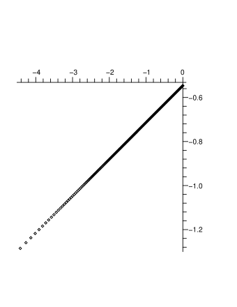
Figure 1. Log-log plot of $|R_{0}|$ as a function of $\lambda$ for $\omega=0$. $R_{0,0}$ is the residue of the pole of $\hat{\psi}(p,x)$ at $p=i$, see Corollary 16.

6. Ionization rate under a short pulse

We now consider a short pulse, with fixed total energy and fixed total number of oscillations. The corresponding Schrödinger equation is

(1) $$i\,\frac{\partial\psi}{\partial t}\,=\Big{(}-\frac{\partial^{2}}{\partial x^{2}}-2\delta(x)+2\lambda\,\delta(x)\,e^{-\lambda t}\cos(\omega t)\Big{)}\,\psi$$

where $\lambda$ is now a large real parameter (note the $\lambda$ in front of the exponential). We are interested in the ionization rate as $\lambda\rightarrow\infty$.

By similar arguments as in §3.5 we have the convergent representation

(2) $$A_{m,n}=\sum_{i=0}^{\infty}(-1)^{i}\left(\frac{\lambda}{2}\right)^{i}\sum_{\tau\in 2^{i}}\prod_{j=0}^{i}B_{n+j,\,m+|\tau^{0}_{j}|}g_{n+i,\,m+|\tau|}$$

Figs. 2 and 3 give $|R_{0,0}|$ (see Corollary 16) and $\lambda$ under different $\omega/\lambda$ ratios. On small scales on the $\lambda$ axis, $|R_{0,0}|$ exhibits rapid oscillations, easier seen if $\omega/\lambda$ is smaller.

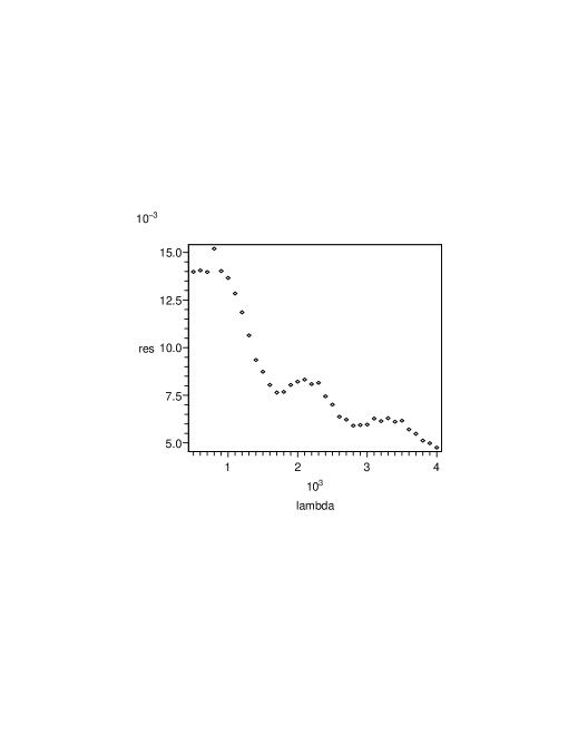
Figure 2. $|R_{0,0}|$ as a function of $\lambda$, with fixed ratio $\omega/\lambda=20$. $R_{0,0}$ is the residue of the pole of $\hat{\psi}(p,x)$ at $p=i$, see Corollary 16.

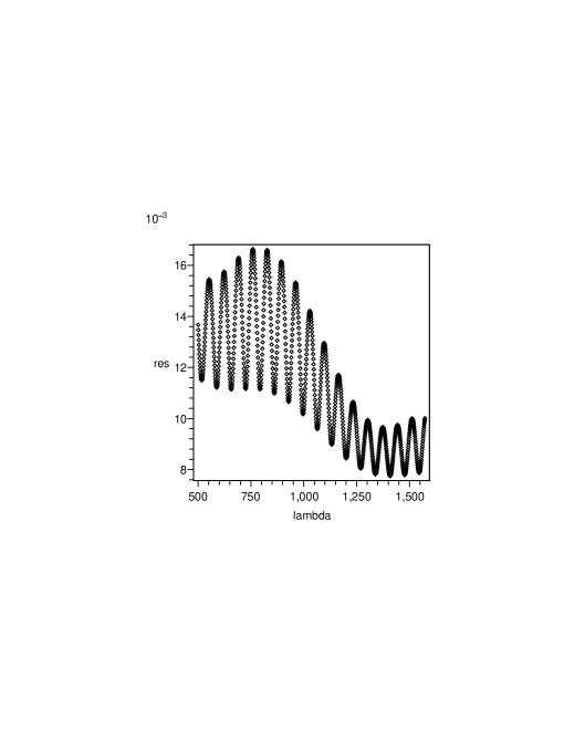
Figure 3. $|R_{0,0}|$ as a function of $\lambda$ when $\omega/\lambda=5$. $R_{0,0}$ is the residue of the pole of $\hat{\psi}(p,x)$ at $p=i$, see Corollary 16.

7. Results for $\lambda=0$ and $\omega\neq 0$

We briefly go over the case $\lambda=0$, where ionization is complete; the full analysis is done in [11]. In this case $\hat{\psi}$ does not have poles on the imaginary line; we give a summary of the argument in [11].

The homogeneous equation now reads

(1) $$\sqrt{\sigma+m\omega}\,A_{m}=-\frac{1}{2}A_{m+1}-\frac{1}{2}A_{m-1}+A_{m}$$

Thus we have

$$\sum_{\mathbb{N}}\sqrt{\sigma+m\omega}\,A_{m}\overline{A_{m}}=-\frac{1}{2}\sum_{\mathbb{N}}A_{m+1}\overline{A_{m}}-\frac{1}{2}\sum_{\mathbb{N}}A_{m-1}\overline{A_{m}}+\sum_{\mathbb{N}}A_{m}\overline{A_{m}}$$

The first sum and the second sum on the right hand side are conjugate to each other, and each term in the third sum is real. So the right hand side is real, thus the left hand side is also real.

For $\Im(\sigma)\neq 0$, $\Im\left(\sqrt{\sigma+m\omega}\,A_{m}\overline{A_{m}}\right)$ has same the sign as $\Im\sigma$. Therefore the sum can not be real and the equation has no nontrivial solution. When $\Im(\sigma)=0$, for $m<0$, all $\Im\left(\sqrt{\sigma+m\omega}\,A_{m}\overline{A_{m}}\right)$ have the same sign and for $m\geq 0$, $\sqrt{\sigma+m\omega}\,A_{m}\overline{A_{m}}$ is real. Since the final sum is purely real, this means $A_{m}=0$ for $m<0$. But then, recursively, all $A_{m}$ should be 0.

Zero is thus the only solution to (1). By the Fredholm alternative the solution $A$ is analytic in $\sqrt{\sigma}$ and thus the associated $y$ is analytic in $\sqrt{\sigma}$. This entails complete ionization.

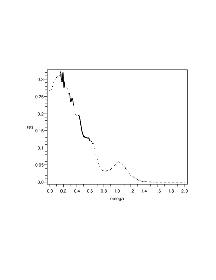
Figure 4. $|R_{0,0}|$, at $\lambda=0.01$, as a function of $\omega$. $R_{0,0}$ is the residue of the pole of $\hat{\psi}(p,x)$ at $p=i$, see Corollary 16.

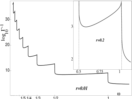
Figure 5. $\log_{10}\Gamma^{-1}$, at $\lambda=0$, as a function of $\omega/\omega_{0}$. $\Gamma$ is the Fermi Golden Rule exponent for the probability decay and $\hbar\omega_{0}=E_{0}$, the energy of the bound state of one delta function of amplitude $r$ [7].

7.1. Small $\lambda$ behavior.

We expect that the behavior of the system at $\lambda=0$ is a limit of the one for small $\lambda$. However, this limit is very singular, as the density of the poles in the left half plane goes to infinity as $\lambda\to 0$, only to become finite for $\lambda=0$. Nonetheless, given a $\lambda$, small but not extremely small, formula (35) allows us to calculate the residue.

Figure 4 shows the behavior of the residue versus $\omega$, for $\lambda=0.01$.

We show for comparison the corresponding result when $\lambda=0$, in Figure 5:

8. Acknowledgments.

This work was supported in part by the National Science Foundation DMS-0601226 and DMS-0600369.

References

- [1] S Agmon Spectral properties of Schrödinger operators and scattering theory, Ann. Scuola. Norm. Sup. Pisa, Ser. IV 2, pp. 151–218 (1975).
- [2] J Belissard, Stability and Instability in Quantum Mechanics, in Trends and Developments in the Eighties (S Albeverio and Ph. Blanchard, ed.) World Scientific, Singapore 1985, pp. 1–106.
- [3] C Bender and S Orszag, Advanced Mathematical Methods for scientists and engineers, McGraw-Hill, 1978, Springer-Verlag 1999.
- [4] C Cohen-Tannoudji, J Duport-Roc and G Arynberg, Atom-Photon Interactions, Wiley (1992).
- [5] O Costin On Borel summation and Stokes phenomena for rank one nonlinear systems of ODE’s Duke Math. J. Vol. 93, No 2: 289–344, 1998
- [6] O Costin, R D Costin and J Lebowitz, “Transition to the continuum of a particle in time-periodic potentials” in Advances in Differential Equations and Mathematical Physics, AMS Contemporary Mathematics series ed. Karpeshina, Stolz, Weikard, and Zeng (2003).
- [7] O Costin, J Lebowitz and A Rokhlenko, Exact Results for the Ionization of a Model Quantum System J. Phys. A: Math. Gen. 33 pp. 1–9 (2000)
- [8] O. Costin, R. D. Costin and J. L. Lebowitz, Time asymptotics of the Schrödinger wave function in time-periodic potentials, Dedicated to Elliott Lieb on the occasion of his 70th birthday, J. Stat. Phys. 1–4 283-310 (2004).1
- [9] O. Costin, J. L. Lebowitz and S. Tanveer On the ionization problem for the Hydrogen atom in time dependent fields (submitted), also available at http://www.math.ohio-state.edu/tanveer
- [10] O Costin, R D Costin, J Lebowitz and A Rokhlenko , Evolution of a model quantum system under time periodic forcing: conditions for complete ionization Comm. Math. Phys. 221, 1 pp 1–26 (2001).
- [11] O Costin, A Rokhlenko and J Lebowitz, On the complete ionization of a periodically perturbed quantum system CRM Proceedings and Lecture Notes 27 pp 51–61 (2001).
- [12] O Costin and A Soffer, Resonance Theory for Schrödinger Operators Commun. Math. Phys. 224 (2001).
- [13] O. Costin, J. L. Lebowitz, A. Rokhlenko, Exact results for the ionization of a model quantum system. J. Phys. A: Math. Gen. 33 6311–6319 (2000).1
- [14] O Costin, R D Costin, J L Lebowitz (in preparation).
- [15] O Costin, R D Costin, Rigorous WKB for discrete schemes with smooth coefficients, SIAM J. Math. Anal. 27, no. 1, 110–134 (1996).
- [16] H L Cycon, R G Froese, W Kirsch and B Simon, Schrödinger Operators, Springer-Verlag (1987).
- [17] J Écalle, Fonctions Resurgentes, Publications Mathematiques D’Orsay, 1981
- [18] J Écalle, in Bifurcations and periodic orbits of vector fields, NATO ASI Series, Vol. 408, 1993
- [19] A Galtbayar, A Jensen and K Yajima, Local time-decay of solutions to Schrödinger equations with time-periodic potentials (J. Stat. Phys., to appear).
- [20] L Hörmander, Linear partial differential operators, Springer (1963).
- [21] J S Howland, Stationary scattering theory for time dependent Hamiltonians. Math. Ann. 207, 315–335 (1974).
- [22] H R Jauslin and J L Lebowitz, Spectral and Stability Aspects of Quantum Chaos, Chaos 1, 114–121 (1991).
- [23] T Kato, Perturbation Theory for Linear Operators, Springer Verlag (1995).
- [24] P D Miller, A Soffer and M I Weinstein, Metastability of Breather Modes of Time Dependent Potentials, Nonlinearity Volume 13 (2000) 507-568.
- [25] C Miranda, Partial differential equations of elliptic type, Springer-Verlag (1970).
- [26] M Reed and B Simon, Methods of Modern Mathematical Physics (Academic Press, New York, 1972).
- [27] A Rokhlenko, O Costin, J L Lebowitz, Decay versus survival of a local state subjected to harmonic forcing: exact results. J. Phys. A: Mathematical and General 35 pp 8943 (2002).
- [28] S Saks and A Zygmund, Analytic Functions, Warszawa-Wroclaw (1952).
- [29] B Simon, Schrödinger Operators in the Twentieth Century, Jour. Math. Phys. 41, 3523 (2000).
- [30] A Soffer and M I Weinstein, Nonautonomous Hamiltonians, Jour. Stat. Phys. 93, 359–391 (1998).
- [31] F Treves, Basic linear partial differential equations, Academic Press (1975).
- [32] W Wasow, Asymptotic expansions for ordinary differential equations, Interscience Publishers (1968).
- [33] K Yajima, Scattering theory for Schrödinger equations with potentials periodic in time, J. Math. Soc. Japan 29 pp 729 (1977)
- [34] K Yajima, Existence of solutions of Schrödinger evolution equations, Commun. Math. Phys. 110 pp 415 (1987).
- [35] A H Zemanian, Distribution theory and transform analysis, McGraw-Hill New York (1965).
- [36] O.Costin Asymptotics and Borel summability, CRC PRESS Boca Raton London New York Washington, D.C.