The distribution of stellar mass in the low-redshift Universe
Abstract
We use a complete and uniform sample of almost half a million galaxies from the Sloan Digital Sky Survey to characterise the distribution of stellar mass in the low-redshift Universe. Galaxy abundances are well determined over almost four orders of magnitude in stellar mass, and are reasonably but not perfectly fit by a Schechter function with characteristic stellar mass and with faint-end slope . For a standard cosmology and a standard stellar Initial Mass Function, only 3.5% of the baryons in the low-redshift Universe are locked up in stars. The projected autocorrelation function of stellar mass is robustly and precisely determined for . Over the range it is extremely well represented by a power law. The corresponding three-dimensional autocorrelation function is . Relative to the dark matter, the bias of the stellar mass distribution is approximately constant on large scales, but varies by a factor of five for . This behaviour is approximately but not perfectly reproduced by current models for galaxy formation in the concordance CDM cosmology. Detailed comparison suggests that a fluctuation amplitude is preferred to the somewhat larger value adopted in the Millennium Simulation models with which we compare our data. This comparison also suggests that observations of stellar mass autocorrelations as a function of redshift might provide a powerful test for the nature of Dark Energy.
keywords:
galaxies: clusters: general – galaxies: distances and redshifts – cosmology: theory – dark matter – large-scale structure of Universe.1 Introduction
Four hundred years ago Galileo turned his telescope to the Milky Way and discovered it to consist of countless faint stars. One hundred and fifty years later, Kant speculated that it might be an enormous, rotating stellar swarm, held together by gravity in a similar way to the Solar System, and that other nebulae might be similar but extremely distant “island universes”. These ideas were finally confirmed when Hubble established the extragalactic distance scale in the 1920’s. Stars were accepted as the dominant form of matter in the Universe from this time until the 1980’s, when new theoretical ideas suggested that the dark matter discovered by Zwicky (1933) might consist of neutral, non-baryonic elementary particles (Cowsik & McClelland, 1973; Peebles, 1982) and X-ray images showed that most of the baryons in rich clusters are in the form of hot, intergalactic gas (Forman & Jones, 1982). It now seems clear that baryons are not the dominant form of matter in our Universe, and that stars account for only a small fraction of the baryons (e.g. Fukugita, Hogan, & Peebles, 1998; Cole et al., 2001; Komatsu et al., 2009). Nevertheless, stars are the only component of the cosmic mix for which a complete and robust census is possible. Such surveys teach us where and with what efficiency baryons were converted into galaxies, and can provide stringent constraints on our general structure formation paradigm.
In recent years it has become clear that stellar masses can be measured for galaxies in a robust way from multi-band photometric measurements of their spectral energy distributions (Bell & de Jong, 2001; Blanton & Roweis, 2007) or from combined photometry and spectroscopy (Kauffmann et al., 2003). Low-mass stars contribute very little to the light of galaxies, so the principal uncertainty in these measurements comes from the stellar Initial Mass Function (IMF). For any particular assumed IMF, the uncertainties due to dust, to metallicity, and to details of the star-formation history turn out to be quite small provided reliable photometry is available out to wavelengths of order 1 micron. Stellar mass is then a more natural way to characterise the number of stars in a galaxy than, for example, B- or K-band luminosity.
In the current paper we use a complete sample of almost half a million galaxies with excellent photometry and accurate redshifts to study the distribution of stellar mass in the low redshift universe. This separates into two parts: the abundance of galaxies as a function of their stellar mass, and the clustering of stellar mass on scales larger than those of individual galaxies. There have been previous studies of the first of these statistics, the so-called mass function of galaxies (e.g. Cole et al., 2001; Bell et al., 2003; Wang et al., 2006; Panter et al., 2007; Baldry et al., 2008). Our results agree with this previous work, though with smaller statistical error bars because of the larger sample (systematic uncertainties due to the IMF remain as large as before, of course).
The second statistic has not, to our knowledge, been estimated previously, although there have been a few measurements of galaxy clustering weighted by stellar light or by dynamical mass (e.g. Boerner et al., 1989). As we show the autocorrelation of stellar mass is remarkable for the accuracy with which it can be estimated from our sample, and for the fact that it turns out to be almost a perfect power law over three orders of magnitude in spatial scale. The near power-law behaviour of galaxy correlations was emphasised in early work (e.g. Davis & Peebles, 1983) and has been examined in some detail in previous studies with Sloan Digital Sky Survey data (e.g. Zehavi et al., 2004, 2005; Masjedi et al., 2006). The latter noted that deviations from a pure power law are detected at high significance in almost all cases. In contrast, our stellar mass autocorrelation does not deviate from the best-fit power law by more than 12.5% for separations between 10 kpc and 10 Mpc, a behaviour which we will show to be partially but not perfectly reproduced by existing galaxy formation models.
The structure of our paper is as follows. In Section 2 we discuss the observational dataset we analyse and the theoretical models with which we compare it. Sections 3 and 4 then present our results for the stellar mass function of galaxies and for the autocorrelation function of stellar mass, respectively. A concluding section discusses these results, compares them with model predictions, and suggests that the shape of the mass autocorrelation function might provide a means to estimate how the cosmic scale factor and the linear growth factor depend on redshift, and hence to constrain the properties of Dark Energy.
2 Data
2.1 SDSS and NYU-VAGC
This study is based on the final data release (DR7; Abazajian et al., 2008) of the Sloan Digital Sky Survey (SDSS; York et al., 2000). This contains images of a quarter of the sky obtained using a drift-scan camera (Gunn et al., 1998) in the u, g, r, i, z bands (Fukugita et al., 1996; Smith et al., 2002; Ivezić et al., 2004), together with spectra of almost a million objects obtained with a fibre-fed double spectrograph (Gunn et al., 2006). Both instruments were mounted on a special-purpose 2.5 meter telescope (Gunn et al., 2006) at Apache Point Observatory. The imaging data are photometrically (Hogg et al., 2001; Tucker et al., 2006) and astrometrically (Pier et al., 2003) calibrated, and were used to select spectroscopic targets for the main galaxy sample (Strauss et al., 2002), the luminous red galaxy sample (Eisenstein et al., 2001), and the quasar sample (Richards et al., 2002). Spectroscopic fibres are assigned to the targets using an efficient tiling algorithm designed to optimise completeness (Blanton et al., 2003). The details of the survey strategy can be found in York et al. (2000) and an overview of the data pipelines and products is provided in the Early Data Release paper (Stoughton et al., 2002). More details on the photometric pipeline can be found in Lupton et al. (2001) and on the spectroscopic pipeline in SubbaRao et al. (2002).
For this paper we take data from Sample dr72 of the New York University Value Added Catalogue (NYU-VAGC)111http://sdss.physics.nyu.edu/vagc/. This is an update of the catalogue constructed by Blanton et al. (2005b) and is based on the full SDSS/DR7 data. Starting from Sample dr72, we construct a magnitude-limited sample of galaxies with and spectroscopically measured redshifts in the range . Here is the -band Petrosian apparent magnitude, corrected for Galactic extinction, and the apparent magnitude limit is chosen in order to get a sample that is uniform and complete over the entire area of the survey. We also restrict ourselves to galaxies located in the main contiguous area of the survey in the northern Galactic cap, excluding the three survey strips in the southern cap (about 10% of the full survey area). These restrictions results in a final sample of 486,840 galaxies.
In addition to the magnitudes, redshifts and positions of the galaxies, the NYU-VAGC provides several other quantities which are needed in our analysis. The first is a stellar mass for each galaxy, which is based on its redshift and the five-band SDSS photometric data, as described in detail in Blanton & Roweis (2007). This estimate corrects implicitly for dust and assumes an universal Initial Mass Function of Chabrier (2003) form. As we demonstrate in Appendix A, once all estimates are adapted to assume the same IMF, the Blanton-Roweis masses agree quite well with those obtained from the simple, single-colour estimator of Bell et al. (2003) and also with those derived by Kauffmann et al. (2003) from a combination of SDSS photometry and spectroscopy. Given the very large sample provided by the SDSS, sampling fluctuations and “cosmic variance” are small. Uncertainties in the mass estimation procedure dominate the systematic error budget for most of the results we present below. Appendix A shows that such uncertainties primarily affect the overall stellar mass scale, as do uncertainties in the IMF itself, as long as it is assumed universal. Results that depend only on the relative stellar masses of galaxies (for example, the stellar mass correlation function) are therefore much more weakly affected than those that depend directly on the mass scale (for example, the mean stellar mass density of the Universe).
The NYU-VAGC also provides the necessary information to correct for incompleteness in our spectroscopic sample. In particular, we use a mask which shows which areas of the sky have been targeted, and which have not, either because they are outside the survey boundary, because they contain a bright confusing source, or because observing conditions were too poor to obtain all the required data. This mask defines the effective area of the survey on the sky, which is 6437 square degrees for the sample we use here. This survey area is divided into a large number of smaller subareas for each of which the NYU-VAGC lists a spectroscopic completeness . This is defined as the fraction of the photometrically defined target galaxies in the subarea for which usable spectra were obtained. The average over our sample galaxies is . Within each subarea the galaxies with spectra can be assumed to be a random sample of all possible targets, with the important exception that fibres cannot be closer than 55 arsec in a single spectroscopic exposure, so that at most one fibre can be placed on a galaxy in a pair or group with smaller angular size than this. (More fibres may be assigned to such clumps if they happen to lie in the overlap region between two or more spectroscopic observations.) It is important to correct for such “fibre collisions” when measuring clustering. As discussed in more detail below, we use the procedures of Li et al. (2006b) and Li et al. (2007) for this purpose. These are based on comparing pair counts as a function of angular separation in the spectroscopic sample and in its parent photometric sample. General incompleteness is dealt with by weighting each galaxy by in all statistical analyses.
A final observational issue is that the SDSS photometric catalogue from which our spectroscopic galaxy sample is drawn is incomplete for low surface brightness galaxies (Blanton et al., 2005a). We discuss this in Appendix B, based on the recent analysis by Baldry et al. (2008), concluding that for our purposes the effects are negligible except possibly at the very lowest stellar masses we study.
2.2 Millennium Simulation, semi-analytic galaxy catalogue, and mock redshift surveys
We have constructed a set of 20 mock SDSS galaxy catalogues from the Millennium Simulation (Springel et al., 2005) using both the sky mask and the magnitude and redshift limits of our real SDSS sample. The Millennium Simulation uses particles to follow the dark matter distribution in a cubic region 500 Mpc on a side. The cosmological parameters assumed are , , , and . Galaxy formation within the evolving dark matter distribution is simulated in postprocessing using semi-analytic methods tuned to give a good representation of the observed low-redshift galaxy population. Our mock catalogues are based on the galaxy formation model of Croton et al. (2006) and are constructed from the publicly available data using the methodology of Li et al. (2006b) and Li et al. (2007). These mock catalogues allow us to derive realistic error estimates for the statistics we measure, including both sampling and cosmic variance uncertainties.
We also use galaxy data from the Millennium Simulation archive222http://www.mpa-garching.mpg.de/millennium to compare and contrast predictions for the total mass and stellar mass correlation functions at and at higher redshift. These data are based on the galaxy formation model of De Lucia & Blaizot (2007).
3 The stellar mass function of galaxies

A first statistic which we can estimate from the data we have available is the abundance of galaxies as a function of their stellar mass. For each observed galaxy we define the quantity to be the maximum redshift at which the observed galaxy would satisfy the apparent magnitude limit of our sample . Evolutionary and K-corrections are included when calculating as described by Li et al. (2006a) and Li et al. (2007). This allows us to define for the galaxy in question as the total comoving volume of the survey out to redshift . The stellar mass function can then be estimated as
| (1) |
where the sum extends over all sample galaxies with stellar mass in the range .
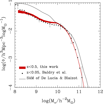
In Figure 1, we show the stellar mass function determined in this way for the galaxies in our sample. The error bars are estimated from the scatter among the mass functions of our 20 mock catalogues. As already noted by Croton et al. (2006) the mass function of this model agrees reasonably well with observation, and indeed the number of galaxies in the real catalogue lies well within the scatter of the numbers found for the 20 mock catalogues. The error bars should thus account correctly for the uncertainties due to sampling and cosmic variance, but they do not include systematic uncertainties in the NYU-VAGC estimates of stellar masses. Appendix A shows that these may be reasonably represented by a dex systematic uncertainty in the overall mass scale. Note that the error bars on neighboring points are strongly correlated.
The mass function of Figure 1 is in good agreement with estimates from the 2dFGRS (Cole et al., 2001) and from earlier releases of the SDSS (e.g. Bell et al., 2003; Wang et al., 2006; Panter et al., 2007; Baldry et al., 2008). In Appendix B we present an explicit comparison with Baldry et al. (2008) which allows us to assess the effect of a small but significant systematic, the incompleteness of the SDSS sample at low mass and low surface brightness. This causes a slight underestimate of abundances below The purely statistical error bars on our mass function are smaller than in earlier work because of the substantially larger size of the sample. It is well determined all the way from up to almost . A fit with a single Schechter function (Schechter, 1976) is not fully consistent with the data. In particular, it significantly underpredicts the abundance of the most massive galaxies. Nevertheless, it provides a reasonable and simple representation of our results. The parameters we obtain, , and are similar to those found in earlier studies. (The errors here are approximate uncertainties in each parameter marginalised over the uncertainties in the other parameters.) Our mass function data can be considerably better represented by fitting three different Schechter functions (i.e. with different parameters) over three disjoint mass ranges. This representation is also plotted on top of the data in Figure 1 and its parameters are listed in Table 1. It provides a compact and accurate summary of our results.
Another useful representation of the stellar mass function is in terms of the percentage points of the cumulative stellar mass distribution. According to our results, half of all the stellar mass in galaxies is in objects with individual stellar mass greater than . The corresponding 5%, 10%, 20%, 80%, 90% and 95% points are , , , , and respectively. (We have used our triple Schechter fit to extrapolate the low-mass end of the mass function when calculating these numbers.) Thus 60% of all stars are in galaxies with stellar mass within a factor of 2.75 of which is about half the stellar mass of the Milky Way. A related characteristic mass which will be of interest below is the mass-weighted mean stellar mass, which can also be thought of as the expected stellar mass of the host of a randomly chosen star. This is and is close to the stellar mass of the Milky Way.
A straightforward integration of our stellar mass function gives the mean comoving stellar mass density of the low-redshift Universe (at , see below). This is , where the error bar is again derived from the scatter among our 20 mock catalogues and so accounts for sampling and cosmic variance effects, but not for systematic errors in the mass determinations of individual galaxies. In the standard concordance cosmology (e.g. Komatsu et al., 2009) only 3.5% of the baryons in the low-redshift Universe are locked up in stars. Clearly, galaxy formation has been a very inefficient process.
| mass range | |||
|---|---|---|---|
| () | (Mpc) | () | |
| 0.0146(5) | -1.13(09) | 9.61(24) | |
| 0.0132(7) | -0.90(04) | 10.37(02) | |
| 0.0044(6) | -1.99(18) | 10.71(04) |
4 stellar mass correlation functions


To obtain a reliable estimate of the clustering of stellar mass, the observed sample must be compared with a “random sample” which is unclustered but fills the same region of the sky and has the same, stellar mass-dependent redshift distribution. We construct our random sample from the observed sample itself, as described in detail in Li et al. (2006a). For each real galaxy we generate 10 sky positions at random within our DR7 mask, and we assign to each of them the properties of the real galaxy, in particular, its values of redshift, stellar mass, and . The validity of the resulting random sample rests on two requirements: 1) the survey area should be large enough that structures in the real sample are wiped out by randomising in angle; 2) the effective depth of the survey must not vary from region to region. Both are true to good accuracy for our sample, which covers deg2, is complete down to and is little affected by foreground dust over the entire survey region. Extensive tests show that random samples constructed in this way produce indistinguishable results from those using the traditional method (Li et al., 2006a). The advantage of this technique in the current application is that it is guaranteed to maintain the complex relation between stellar mass and photometric properties (and thus sample selection criteria) which holds in the real data.
We begin by estimating the redshift-space, stellar mass correlation function, using an appropriate version of the Landy & Szalay (1993) estimator:
| (2) |
where the data-data, data-random and random-random pair counts are weighted as follows:
| (3) |
| (4) |
| (5) |
where the sums are over all pairs of the relevant type (, or ) with separations in the two-dimensional separation bin labelled by and , the pair separations perpendicular and parallel to the line of sight. Note that in the and sums each pair appears twice (as and ). In these expressions, and are the stellar masses of the members of each pair, and are their associated spectroscopic completeness fractions, and is the volume over which both galaxies would be included in the sample. To reduce sampling noise, random samples are usually constructed with many more particles than the real sample. To normalise appropriately, needs to be multiplied by and by where and are the numbers of galaxies in the real and random samples, respectively. In our case, .
The final weight in the above equations is the factor which appears in the data-data counts only. This is a function of the angular separation of the two galaxies, and is defined as the fraction of pairs of angular separation which are missing from our spectroscopic sample as a direct consequence of the fibre collision problem. We estimate this fraction in the same way as Li et al. (2006b) and Li et al. (2007). We calculate angular correlation functions for the spectroscopic sample and for its parent photometric sample, and we then define
| (6) |
Detailed tests of this procedure can be found in Li et al. (2006b).

Rather than analysing these two-dimensional correlation estimates, we integrate over the line-of-sight separation to obtain an estimate of the projected stellar mass correlation function, . This function is independent of redshift-space distortions and is related by a simple integral transform to the three-dimensional spatial autocorrelation function for stellar mass . Thus we take
| (7) |
where we choose Mpc as the outer limit for the depth integration (in order to limit noise from distant uncorrelated regions) so that the summation for computing runs from h-1 Mpc to h-1 Mpc, given that we use bins of width h-1 Mpc.
The measurements of obtained in this way are plotted as triangles in the top panel of Figure 2. Error bars are estimated from the scatter between estimates of made by applying exactly the same procedures to our 20 mock SDSS samples. We have also estimated error bars by bootstrap resampling of the SDSS data themselves. As shown in Figure 3, these two methods produce consistent results on small scales () but at larger separations the bootstrap estimates are consistently smaller than those obtained from the mock catalogues. This is because the former do not account properly for cosmic variance, which is the primary source of uncertainty on large scales. Over the range the measurements have errors below 10% and are remarkably well approximated by a power law. The rms scatter around the power law shown in the figure is only 6.9% over this range. At larger separations rolls off below the extrapolation of the power law. A similar result with a slightly but significantly shallower power law index was obtained by Hawkins et al. (2003) for galaxies (rather than stellar mass) in the 2dF Galaxy Redshift Survey, and only quite subtle deviations from power laws are seen in earlier SDSS measurements of galaxy correlations (e.g. Zehavi et al., 2004, 2005; Masjedi et al., 2006) This in turn echoes the very first galaxy correlation results obtained by Totsuji & Kihara (1969), Peebles (1974) and Davis & Peebles (1983).

For comparison, Figure 2 also shows predictions for the corresponding projected 2PCF for dark matter, , obtained from the snapshot of the Millennium Simulation (as we show below, this is the appropriate mean depth for our SDSS measurement). A maximum line-of-sight depth of 40 was adopted when computing this statistic in order to mimic our SDSS procedures. The result, plotted as a solid line in the top panel of the figure, shows much more pronounced features than stellar mass correlation function. The ratio between them is shown in the lower two panels, and can be thought of as an estimate of the scale-dependent bias between stars and dark matter. Our results are consistent with bias being independent of scale at , but the scale-dependence at smaller separations is strong, with a total range of a factor of 5.
In order to interpret the stellar mass autocorrelation function of Figure 2 it is helpful to see how the contributions to our estimate are distributed in redshift and across galaxies of differing individual stellar mass. Figure 4 illustrates the distribution in redshift. The solid curve histograms contributions to Equ. 3 from pairs with and . The median of this distribution is and the 10 and 90% points are and , respectively. (These results are very insensitive to the particular range chosen.) For comparison, the dotted line is a redshift histogram for all galaxies in our spectroscopic sample and has median at , and 10 and 90% points at and 0.16, while the dashed line is the histogram of contributions to our estimate of the cosmic stellar mass density (i.e. for galaxy at redshift ) with median at , and 10 and 90% points at and 0.16. The autocorrelation function is dominated by contributions from a narrower redshift range and peaking at lower redshift than is the parent sample or the stellar density estimate we derived from it. It is also remarkable that although our sample includes almost half a million galaxies and covers a sixth of the sky, the histograms of Figure 4 still show strong features which reflect large-scale structure. Our mock catalogues show that features at this level, although striking, are expected and do not appreciably affect our estimate of .
Figure 5 shows contributions to our estimate of histogrammed as a function of the stellar mass of the most massive (solid line) and of the least massive (dashed line) galaxy in each pair. As was the case for the redshift distributions, we find these curves to be almost independent of the range used; here we again use pairs with and . For comparison, we also show a histogram of contributions to our estimate of the cosmic stellar mass density as a function of the stellar mass of the individual galaxies. This is effectively the stellar mass function of Figure 1, multiplied by and plotted on a linear scale. In all three cases, the dominant contributions come from a relatively narrow range of stellar mass centred quite close to the mass of the Milky Way. The autocorrelations are dominated by contributions from galaxies in an even narrower mass range than those dominating the cosmic stellar mass density, by pairs quite similar to the Local Group.
5 Discussion
Our estimates of the mean stellar mass density and of the stellar mass autocorrelation function allow us to calculate the average stellar mass within distance of a randomly chosen star. This is
where the constant , the mean stellar mass of the chosen star’s own galaxy, was calculated from the stellar mass function in section 3. The second and third terms account for stars in other galaxies. It is interesting that these terms become comparable to only at . This is at least thirty times the size of the stellar component of a typical galaxy, a factor which quantifies how much dissipative effects have condensed the visible components of galaxies with respect to the larger scale dissipationless hierarchy.
It is striking that our measured stellar-mass autocorrelation function is very well fit by a power law over about three orders of magnitude in spatial scale. This behaviour breaks down dramatically on smaller scales where “one-galaxy” contributions cause to jump in amplitude by about two orders of magnitude (see equation (5)) but also on larger scales where we detect the roll-down in amplitude expected in CDM universes. When it was first seen in galaxy autocorrelations, such power-law behaviour was interpreted as evidence for the scale-free nature of hierarchical clustering under gravity (e.g. Peebles, 1980). High-quality numerical simulations have improved our understanding of this process considerably, showing that precise power-law behaviour should not be expected, either on highly nonlinear scales or in the transition between linear and nonlinear scales. Fig. 2 shows dark matter correlations in the Millennium Simulation to depart substantially from power-law behaviour in both these regimes. It is thus surprising that the observed stellar mass autocorrelation is an excellent power law between 10kpc and 10Mpc. In our standard structure formation model, this must be seen as a coincidence. Different processes are required to cause convergence towards the observed power law on different scales.
We use the Millennium Simulation to explore this issue further in Figure 6. This compares projected stellar and dark matter autocorrelation functions at and 3.0 using the semi-analytic model of De Lucia & Blaizot (2007) to specify the stellar masses of the “galaxies”. The upper panel shows the dark and stellar mass autocorrelations separately, while the lower panel shows their ratio, the “bias factor”, as a function of scale. The well-known result that galaxy correlations are predicted to evolve much more weakly than dark matter correlations is very clear in this plot. More interesting in the current context is the fact that the predicted stellar mass correlations are much closer to a power law for Mpc than are those for the dark matter, although the deviations are significantly larger than in the real data of Fig. 2. The two can be compared in the lower panel of Fig. 6 where the SDSS bias data are shown as symbols with error bars. Although the model reproduces the “two-halo” part of the observed function very well, it overpredicts the “one-halo” part by about 50% and this leads to the bulge above a power law which is visible in the upper panel. At higher redshifts the model stellar mass autocorrelations maintain their power-law behaviour on small scales, becoming even steeper than at . By the transition between one and two halo terms has become very obvious. This reinforces the conclusion that the remarkably precise power law of Fig. 2 is just a coincidence.


Another interesting feature of the model bias curves in Fig. 6 is the fact that they are smooth and almost constant over the range . They show at most a very weak feature at the transition between the 1-halo and 2-halo regimes, despite the fact that the projected correlation functions from which they were derived show such features quite clearly. In contrast, when we divide our featureless observed by the corresponding function for dark matter in the Millennium Simulation, the resulting bias curve shows an obvious step at the 1-halo/2-halo transition which reflects the marked change in slope of the dark matter correlations at this point (see the bottom panel of Fig. 2). This suggests that the amplitude of mass fluctuations is too high in the Millennium Simulation, and that the shape of our stellar mass correlation function can be used to estimate the value of the fluctuation amplitude parameter .
We illustrate this possibility in Fig. 7 where we use the projected dark matter correlations measured in the Millennium Simulation at redshifts of 0.32, 0.62 and 0.99 to represent those expected at in cosmologies with identical parameters except that is reduced to 0.8, 0.7 and 0.6 respectively333This scaling assumes that the nonlinear dark matter power spectrum depends on the shape of the linear power spectrum and its extrapolated amplitude, but not on other parameters such as or . This approximation is quite good over the range of scales relevant here, and is certainly good enough for the present, essentially qualitative argument.. We derive bias functions from our SDSS stellar mass correlations using these three functions in addition to the original data, and we compare their shapes to those of model bias functions at and 3 taken from Fig. 6. For the 1-halo/2-halo transition feature is clear and is much larger than any feature seen in the models. For the feature has reversed sign and the inferred bias function has a much more marked overall slope than any of the models. The “Goldilocks” solution appears to be close to where the bias function is quite flat and the transition feature is almost absent. This accords quite well with the values of suggested by joint analysis of WMAP5 and low-redshift supernova and BAO data (Komatsu et al., 2009).
If it can be shown that the smooth behaviour of the model bias functions of Fig. 7 is generic to all physically reasonable CDM galaxy formation models, then these results suggest a powerful cosmological test. Projected stellar mass correlation functions can be estimated as a function of redshift from any large galaxy survey with sufficiently good photometry to obtain robust and relatively precise photometric redshifts. The 1-halo/2-halo feature typically occurs at radii where these correlation function estimates have their best signal-to-noise, and thus is much easier to measure than, say, the baryon oscillation feature. Requiring the bias functions to be smooth and nearly flat will determine . In addition, the location of the transition feature in the individual correlation functions provides a length-scale which can be used to get an angular size distance to each redshift. If it works. this scheme thus provides measurements of both the functions of redshift which are needed to constrain the nature of Dark Energy.
Although the De Lucia & Blaizot (2007) galaxy catalogue provides a surprisingly good fit to the observed clustering of stellar mass, it does much less well when compared to the stellar mass function of Fig. 1. The very small error bars highlight discrepancies which could be ignored when comparing to previously published and less precise mass functions. The most important of these concerns the abundances at low mass, where the SDSS measurements are a factor of two below the galaxy formation models implemented on the Millennium Simulation over the full range (see Fig. 11 below). Clearly, galaxy formation in low-mass halos was considerably less efficient in the real Universe than these models predict. Precise statistics for the distribution of stellar mass of the kind obtained in this paper provide hard constraints for galaxy formation models, and learning what is required to fit them properly may teach us much about the physics of galaxy formation.
Acknowledgments
We thank the referee for helpful comments and Michael Blanton for help in understanding the stellar mass estimates in NYU-VAGC. CL is supported by the Joint Postdoctoral Programme in Astrophysical Cosmology of Max Planck Institute for Astrophysics and Shanghai Astronomical Observatory, by NSFC (10533030, 10633020), by 973 Program (No.2007CB815402) and by the Knowledge Innovation Program of CAS (No.KJCX2-YW-T05).
Funding for the SDSS and SDSS-II has been provided by the Alfred P. Sloan Foundation, the Participating Institutions, the National Science Foundation, the U.S. Department of Energy, the National Aeronautics and Space Administration, the Japanese Monbukagakusho, the Max Planck Society, and the Higher Education Funding Council for England. The SDSS Web Site is http://www.sdss.org/.
The SDSS is managed by the Astrophysical Research Consortium for the Participating Institutions. The Participating Institutions are the American Museum of Natural History, Astrophysical Institute Potsdam, University of Basel, University of Cambridge, Case Western Reserve University, University of Chicago, Drexel University, Fermilab, the Institute for Advanced Study, the Japan Participation Group, Johns Hopkins University, the Joint Institute for Nuclear Astrophysics, the Kavli Institute for Particle Astrophysics and Cosmology, the Korean Scientist Group, the Chinese Academy of Sciences (LAMOST), Los Alamos National Laboratory, the Max-Planck-Institute for Astronomy (MPIA), the Max-Planck-Institute for Astrophysics (MPA), New Mexico State University, Ohio State University, University of Pittsburgh, University of Portsmouth, Princeton University, the United States Naval Observatory, and the University of Washington.
References
- Abazajian et al. (2008) Abazajian K., et al., 2008, ApJS, 182, 543
- Adelman-McCarthy et al. (2006) Adelman-McCarthy J. K., et al., 2006, ApJS, 162, 38
- Baldry et al. (2008) Baldry I. K., Glazebrook K., Driver S. P., 2008, MNRAS, 388, 945
- Bell & de Jong (2001) Bell E. F., de Jong R. S., 2001, ApJ, 550, 212
- Bell et al. (2003) Bell E. F., McIntosh D. H., Katz N., Weinberg M. D., 2003, ApJS, 149, 289
- Bernardi et al. (2007) Bernardi M., Hyde J. B., Sheth R. K., Miller C. J., Nichol R. C., 2007, AJ, 133, 1741
- Blanton et al. (2003) Blanton M. R., Lin H., Lupton R. H., Maley F. M., Young N., Zehavi I., Loveday J., 2003, AJ, 125, 2276
- Blanton & Roweis (2007) Blanton M. R., Roweis S., 2007, AJ, 133, 734
- Blanton et al. (2005a) Blanton M. R., Lupton R. H., Schlegel D. J., Strauss M. A., Brinkmann J., Fukugita M., Loveday J., 2005a, ApJ, 631, 208
- Blanton et al. (2005b) Blanton M. R., Schlegel D. J., Strauss M. A., Brinkmann J., Finkbeiner D., Fukugita M., Gunn J. E., Hogg D. W., et al.,, 2005b, AJ, 129, 2562
- Boerner et al. (1989) Boerner G., Mo H., Zhou Y., 1989, A&A, 221, 191
- Chabrier (2003) Chabrier G., 2003, PASP, 115, 763
- Cole et al. (2001) Cole S., Norberg P., Baugh C. M., Frenk C. S., Bland-Hawthorn J., Bridges T., Cannon R., Colless M., et al.,, 2001, MNRAS, 326, 255
- Cowsik & McClelland (1973) Cowsik R., McClelland J., 1973, ApJ, 180, 7
- Croton et al. (2006) Croton D. J., Springel V., White S. D. M., De Lucia G., Frenk C. S., Gao L., Jenkins A., Kauffmann G., et al.,, 2006, MNRAS, 365, 11
- Davis & Peebles (1983) Davis M., Peebles P. J. E., 1983, ApJ, 267, 465
- De Lucia & Blaizot (2007) De Lucia G., Blaizot J., 2007, MNRAS, 375, 2
- Eisenstein et al. (2001) Eisenstein D. J., Annis J., Gunn J. E., Szalay A. S., Connolly A. J., Nichol R. C., Bahcall N. A., Bernardi M., et al.,, 2001, AJ, 122, 2267
- Forman & Jones (1982) Forman W., Jones C., 1982, ARA&A, 20, 547
- Fukugita, Hogan, & Peebles (1998) Fukugita M., Hogan C. J., Peebles P. J. E., 1998, ApJ, 503, 518
- Fukugita et al. (1996) Fukugita M., Ichikawa T., Gunn J. E., Doi M., Shimasaku K., Schneider D. P., 1996, AJ, 111, 1748
- Gallazzi et al. (2005) Gallazzi A., Charlot S., Brinchmann J., White S. D. M., Tremonti C. A., 2005, MNRAS, 362, 41
- Glazebrook et al. (2004) Glazebrook K., et al., 2004, Nature, 430, 181
- Gunn et al. (1998) Gunn J. E., Carr M., Rockosi C., Sekiguchi M., Berry K., Elms B., de Haas E., Ivezić Ž., et al.,, 1998, AJ, 116, 3040
- Gunn et al. (2006) Gunn J. E., Siegmund W. A., Mannery E. J., Owen R. E., Hull C. L., Leger R. F., Carey L. N., Knapp G. R., et al.,, 2006, AJ, 131, 2332
- Hawkins et al. (2003) Hawkins E., Maddox S., Cole S., Lahav O., Madgwick D. S., Norberg P., Peacock J. A., Baldry I. K., et al.,, 2003, MNRAS, 346, 78
- Hogg et al. (2001) Hogg D. W., Finkbeiner D. P., Schlegel D. J., Gunn J. E., 2001, AJ, 122, 2129
- Ivezić et al. (2004) Ivezić Ž., Lupton R. H., Schlegel D., Boroski B., Adelman-McCarthy J., Yanny B., Kent S., Stoughton C., et al.,, 2004, Astronomische Nachrichten, 325, 583
- Kauffmann et al. (2003) Kauffmann G., Heckman T. M., White S. D. M., Charlot S., Tremonti C., Brinchmann J., Bruzual G., Peng E. W., et al.,, 2003, MNRAS, 341, 33
- Komatsu et al. (2009) Komatsu E., Dunkley J., Nolta M. R., Bennett C. L., Gold B., Hinshaw G., Jarosik N., Larson D., et al.,, 2009, ApJS, 180, 330
- Kroupa (2001) Kroupa P., 2001, MNRAS, 322, 231
- Landy & Szalay (1993) Landy S. D., Szalay A. S., 1993, ApJ, 412, 64
- Lauer et al. (2007) Lauer T. R., et al., 2007, ApJ, 662, 808
- Li et al. (2007) Li C., Jing Y. P., Kauffmann G., Börner G., Kang X., Wang L., 2007, MNRAS, 376, 984
- Li et al. (2006a) Li C., Kauffmann G., Jing Y. P., White S. D. M., Börner G., Cheng F. Z., 2006a, MNRAS, 368, 21
- Li et al. (2006b) Li C., Kauffmann G., Wang L., White S. D. M., Heckman T. M., Jing Y. P., 2006b, MNRAS, 373, 457
- Lupton et al. (2001) Lupton R., Gunn J. E., Ivezić Z., Knapp G. R., Kent S., 2001, in Astronomical Data Analysis Software and Systems X, Harnden Jr. F. R., Primini F. A., Payne H., eds., Vol. 238, pp. 269–+
- Masjedi et al. (2006) Masjedi M., Hogg D. W., Cool R. J., Eisenstein D. J., Blanton M. R., Zehavi I., Berlind A. A., Bell E. F., et al.,, 2006, ApJ, 644, 54
- Panter et al. (2007) Panter B., Jimenez R., Heavens A. F., Charlot S., 2007, MNRAS, 378, 1550
- Peebles (1974) Peebles P. J. E., 1974, ApJ, 189, L51+
- Peebles (1980) —, 1980, The large-scale structure of the universe. Research supported by the National Science Foundation. Princeton, N.J., Princeton University Press, 1980. 435 p.
- Peebles (1982) —, 1982, ApJ, 258, 415
- Pier et al. (2003) Pier J. R., Munn J. A., Hindsley R. B., Hennessy G. S., Kent S. M., Lupton R. H., Ivezić Ž., 2003, AJ, 125, 1559
- Richards et al. (2002) Richards G. T., Fan X., Newberg H. J., Strauss M. A., Vanden Berk D. E., Schneider D. P., Yanny B., Boucher A., et al.,, 2002, AJ, 123, 2945
- Schechter (1976) Schechter P., 1976, ApJ, 203, 297
- Smith et al. (2002) Smith J. A., Tucker D. L., Kent S., Richmond M. W., Fukugita M., Ichikawa T., Ichikawa S.-i., Jorgensen A. M., et al.,, 2002, AJ, 123, 2121
- Springel et al. (2005) Springel V., White S. D. M., Jenkins A., Frenk C. S., Yoshida N., Gao L., Navarro J., Thacker R., et al.,, 2005, Nature, 435, 629
- Stoughton et al. (2002) Stoughton C., Lupton R. H., Bernardi M., Blanton M. R., Burles S., Castander F. J., Connolly A. J., Eisenstein D. J., et al.,, 2002, AJ, 123, 485
- Strauss et al. (2002) Strauss M. A., Weinberg D. H., Lupton R. H., Narayanan V. K., Annis J., Bernardi M., Blanton M., Burles S., et al.,, 2002, AJ, 124, 1810
- SubbaRao et al. (2002) SubbaRao M., Frieman J., Bernardi M., Loveday J., Nichol B., Castander F., Meiksin A., 2002, in Society of Photo-Optical Instrumentation Engineers (SPIE) Conference Series, Starck J.-L., Murtagh F. D., eds., Vol. 4847, pp. 452–460
- Totsuji & Kihara (1969) Totsuji H., Kihara T., 1969, PASJ, 21, 221
- Tucker et al. (2006) Tucker D. L., Kent S., Richmond M. W., Annis J., Smith J. A., Allam S. S., Rodgers C. T., Stute J. L., et al.,, 2006, Astronomische Nachrichten, 327, 821
- von der Linden et al. (2007) von der Linden A., Best P. N., Kauffmann G., White S. D. M., 2007, MNRAS, 379, 867
- Wang et al. (2006) Wang L., Li C., Kauffmann G., De Lucia G., 2006, MNRAS, 371, 537
- York et al. (2000) York D. G., Adelman J., Anderson Jr. J. E., Anderson S. F., Annis J., Bahcall N. A., Bakken J. A., Barkhouser R., et al.,, 2000, AJ, 120, 1579
- Zehavi et al. (2004) Zehavi I., Weinberg D. H., Zheng Z., Berlind A. A., Frieman J. A., Scoccimarro R., Sheth R. K., Blanton M. R., et al.,, 2004, ApJ, 608, 16
- Zehavi et al. (2005) Zehavi I., Zheng Z., Weinberg D. H., Frieman J. A., Berlind A. A., Blanton M. R., Scoccimarro R., Sheth R. K., et al.,, 2005, ApJ, 630, 1
- Zwicky (1933) Zwicky F., 1933, Helvetica Physica Acta, 6, 110
Appendix A Systematic biases due to the stellar mass definition
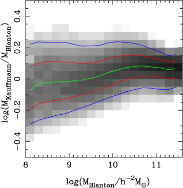
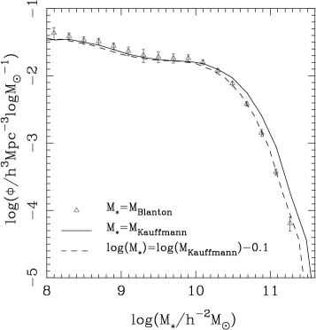

In order to explore possible systematics in our results due to the particular Blanton & Roweis (2007) stellar mass estimates we have used, we here repeat parts of our analysis using both the spectroscopy-photometry-based stellar masses of Kauffmann et al. (2003), , and the simpler colour-magnitude-based stellar masses of Bell et al. (2003), .
For we have had to go back to the Sample dr4 of NYU-VAGC, which is based on SDSS Data Release 4 (DR4; Adelman-McCarthy et al., 2006), since is not available for later releases. From Sample dr4 we have selected a sample of 300,596 galaxies using the same criteria as in § 2.1. Measurements of are taken from the MPA/JHU SDSS DR4 database444http://www.mpa-garching.mpg.de/SDSS/DR4/. The reader is referred to Kauffmann et al. (2003) for a detailed description of the methodology used to derive . In brief, the amplitude of the 4000-Å break and the strength of the H absorption line were obtained from stellar population synthesis models for a library of 32,000 diverse star formation histories. A maximum-likelihood estimate of the -band stellar mass-to-light ratio can then be estimated for each galaxy from its observed and H indices and applied to its observed -band luminosity to estimate its stellar mass.
The upper panel of Figure 8 shows a galaxy-by-galaxy comparison of to , the stellar mass estimate used in the main part of this paper, as a function of . As already shown in Blanton & Roweis 2007 (see their Fig. 17), the two estimates are very similar, with a typical scatter of 0.1 dex and with offsets below dex at all . The median of , , as a function of can be well represented by a hyperbolic tangent function,
| (9) |
which we show as a dotted line in the figure.
In the lower panel of Figure 8, the stellar mass function estimated from is plotted as a solid line, and is compared to that from shown as triangles. Both estimates are based on DR4 so the function differs from that of Figure 1. Error bars on the latter show the scatter between 20 mock catalogues constructed from the Millennium Simulation using the same sky mask, magnitude and redshift limits as for the real DR4 sample, as described in § 2.2. The two mass functions are consistent with each other at masses below . At higher masses, -based mass function lies above that based on . This difference almost disappears if the former is shifted to the left by as shown by the dashed line. With this small shift in mass scale, the difference in abundance between the two determinations nowhere exceeds 0.1 dex.
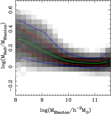
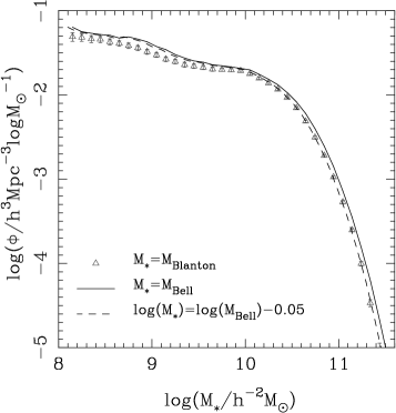
We now consider . Here we use the DR7 data as in the main text and we compute for each galaxy from its colour and its -band luminosity using the formulae given by Bell et al. (2003, see their Appendix 2 and Table 7) for a Kroupa IMF (Kroupa, 2001). This is the IMF adopted by Kauffmann et al. (2003) and it is quite similar to the Chabrier IMF assumed by Blanton & Roweis (2007).
Figure 9 is identical in format to Figure 8. The upper panel is a direct galaxy-by-galaxy comparison of and , while the lower panel compares DR7 mass functions obtained with the two stellar mass estimates The symbols and lines have the same meaning as in the previous figure. The median mass ratio is almost independent of at masses above , but it increases substantially at lower masses, reaching 0.3 dex at . This behaviour can be modelled by a quartic function,
| (10) |
where and . With a scale shift of , the stellar mass function based on is a good match to that based on at masses above , but is high by dex at lower masses.
In summary, differences between these three observational estimators of stellar mass affect our mass function determination primarily through small off-sets in the mass scale. Once this is taken into account, abundance offsets between the different estimates are quite small across the full range that we consider. As we now demonstrate, effects on our stellar mass autocorrelation function estimate are much smaller.
In Figure 10 we plot the ratio of the stellar mass autocorrelation function computed using to that computed using . The two measurements are indistinguishable on scales above about 30 kpc. For kpc, the amplitude of the -based correlation function is slightly higher, but still within the error bars of the measurements. This can be understood from the fact that, as shown in Figure 5, the mass autocorrelations are dominated by contributions from galaxies in a relatively narrow mass range where Figures 8 and 9 show the scatter between the various estimators to be small. Any scale off-set between them drops out in the definition of the autocorrelation function.
Appendix B Incompleteness for low surface brightness galaxies
As discussed by Blanton et al. (2005a) the SDSS galaxy samples are incomplete for low surface brightness (SB) objects. This affects a negligible fraction of high-mass galaxies but can become serious for dwarfs. Thus one may be concerned that our stellar mass functions underestimate the abundance of low-mass galaxies. Baldry et al. (2008) have examined this issue in some detail, deriving the bivariate distribution of SDSS galaxies in SB and stellar mass. They found that for the stellar masses studied here, the distribution of is approximately gaussian at given stellar mass, with a mean which decreases linearly with over the range to and a scatter which increases slightly towards lower masses (see their Fig.4). As stellar mass decreases, the fraction of galaxies with SB below the SDSS completeness limit thus steadily increases. Nevertheless, at the lower limit to which we plot our mass function ( in Fig. 4 of Baldry et al. (2008) since they adopt ) the estimated completeness is still well above 70%. We therefore expect incompleteness to have at most a minor effect on our results.
In Figure 11 we compare our DR7 stellar mass function explicitly to the one which Baldry et al. (2008) estimated for DR4 galaxies at . Baldry et al. (2008) used stellar masses estimated as the average of those obtained by four different published methods (Kauffmann et al., 2003; Glazebrook et al., 2004; Gallazzi et al., 2005; Panter et al., 2007). In the mean this should give a mass scale close to that of Blanton & Roweis (2007). Because of the substantially smaller volume of their sample, the Baldry et al. (2008) results are substantially noisier than our own. (In order to include cosmic variance effects, we have derived the error bars in the figure from mock catalogues in a similar way to those shown on our own mass functions in the main body of our paper.) Agreement is very good over the full mass range plotted. Furthermore, the analysis in their paper shows that SB incompleteness affects only the two or three lowest mass points plotted in Figure 11 and so is negligible for our purposes. This figure also shows the stellar mass function of the Millennium Simulation galaxy formation model of De Lucia & Blaizot (2007). This agrees well with the observations around the knee of the function, but it predicts the rarest and most massive galaxies to have stellar masses 0.2 dex larger than those estimated in SDSS, and, as noted in the final paragraph of our main text, it predicts an abundance of low-mass galaxies which is substantially larger than observed.
Finally we note that SB incompleteness has no effect on the stellar mass autocorrelations that we estimate because, as we show in Figure 5, these are dominated by contributions from galaxies of substantially larger stellar mass.