Spin Density Matrix Elements in Exclusive $\rho^{0}$ Electroproduction on ¹H and ²H Targets at 27.5 GeV Beam Energy

Abstract

Spin Density Matrix Elements (SDMEs) describing the angular distribution of exclusive $\rho^{0}$ electroproduction and decay are determined in the HERMES experiment with 27.6 GeV beam energy and unpolarized hydrogen and deuterium targets. Eight (fifteen) SDMEs that are related (unrelated) to the longitudinal polarization of the beam are extracted in the kinematic region $1~{}\rm{GeV}^{2}<Q^{2}<7$ GeV², $3.0~{}{\rm GeV}<W<6.3$ GeV, and $-t<0.4$ GeV². Within the given experimental uncertainties, a hierarchy of relative sizes of helicity amplitudes is observed. Kinematic dependences of all SDMEs on $Q^{2}$ and $t$ are presented, as well as the longitudinal-to-transverse $\rho^{0}$ electroproduction cross section ratio as a function of $Q^{2}$. A small but statistically significant deviation from the hypothesis of $s$-channel helicity conservation is observed. An indication is seen of a contribution of unnatural-parity-exchange amplitudes; these amplitudes are naturally generated with a quark-exchange mechanism.

1 Introduction

In exclusive production of vector mesons such as $\rho$, $\omega$ or $\phi$ from deep-inelastic lepton scattering (see Fig. 1), measurements of angular and momentum distributions of the scattered lepton and vector meson decay products allow one to study the production mechanism and, in a model-dependent way, the structure of the nucleon.

For more than 40 years, many basic features of vector meson production by a virtual photon have been successfully explained in terms of the Vector Meson Dominance (VMD) model vmd1 ; vmd2 . In this model, the virtual photon fluctuates into a vector meson whose interaction with the nucleon could be described, for example, using Regge phenomenology. More recently, in the context of perturbative Quantum Chromo-Dynamics (pQCD), exclusive meson production at sufficiently large values of the photon virtuality $Q^{2}$ and the invariant mass of the photon-nucleon system $W$ is assumed to be dominated by so-called handbag-diagrams (see Fig. 2) that involve various non-perturbative nucleon structure functions, known as Generalized Parton Distributions (GPDs) gpd1 ; gpd2 ; gpd3 ; strikman .

Figure 1: A generic $t$-channel exchange process for $\gamma^{\star}N\rightarrow\rho^{0}N^{\prime}$. Each particle’s four-momentum is denoted in parentheses.

In pQCD, the common model of the production of vector mesons at high $Q^{2}$ and $W$ can be considered as three consecutive steps brodsk : i) dissociation of the virtual photon into a quark-antiquark ($q\bar{q}$) pair, ii) scattering of the pair on a nucleon (nucleus), iii) formation of the observed vector meson from the $q\bar{q}$-pair. (A full quantum mechanical treatment includes all possible time orderings, which may be more important at lower energies.) The interaction of the $q\bar{q}$-pair with the nucleon can proceed via two distinct mechanisms. The first one, two-gluon exchange, is described by the Feynman diagram shown in Fig. 2a. This process transfers the same quantum numbers as pomeron exchange in the Regge picture, and is anticipated to exhibit a similar phenomenology. The second mechanism is described by the exchange of a $q\bar{q}$-pair, also possibly with additional gluons connecting them, and is called quark-exchange (Fig. 2b). The corresponding process in Regge phenomenology iwing is the exchange of “secondary” reggeons, such as $\rho$, $\omega$, $f_{2}$ and $a_{2}$ in the case of natural-parity exchange (NPE), in which the spin $J$ and parity $P$ associated with the reggeon trajectory are $J^{P}=0^{+},1^{-},2^{+},...$, or $\pi$, $a_{1}$, $b_{1}$ mesons with $J^{P}=0^{-},1^{+},...$ in the case of “unnatural-parity” exchange (UPE). In the GPD formalism, NPE (UPE) processes are described by $H$ and $E$ ($\widetilde{H}$ and $\widetilde{E}$) GPDs. In the intermediate energy range of the HERMES experiment ($3~{}\rm{GeV}<W<6$ GeV) and the moderate values of photon virtuality ($1~{}\rm{GeV}^{2}<Q^{2}<7$ GeV²) both Regge phenomenology and pQCD may be applied to describe exclusive vector meson production. The interpretations they offer of the experimental data are often complementary, although not necessarily consistent.

The main focus of this work is on the measurement of Spin Density Matrix Elements (SDMEs) of the $\rho^{0}$ meson, which describe the distribution of final spin states of this produced vector meson. These elements depend on amplitudes for the angle- and momentum-dependent transition processes between initial spin states of the virtual photon and final spin states of the produced vector meson. The values of SDMEs serve to establish the hierarchy of helicity amplitudes that are commonly used to describe exclusive $\rho^{0}$ production. In this way the relative importance of the various $\gamma^{*}\to\rho^{0}$ transitions is revealed. Two main ordering principles are observed in vector meson leptoproduction, $s$-channel helicity conservation (SCHC) and the dominance of NPE over UPE mechanisms. SCHC implies that only $\gamma^{*}\rightarrow\rho^{0}$ transitions with the same helicities of virtual photon and $\rho^{0}$ occur in the reaction when considered in the “hadronic” center-of-mass frame (defined below). These concepts apply both in the reggeon-exchange picture and in pQCD. In particular, we note that a signal of UPE is evidence of quark-antiquark exchange (Fig. 2b), as the pomeron has natural parity.

At high energies pomeron exchange dominates, and secondary-reggeon exchanges with natural parity are suppressed by a factor $\sim M/W$ iwing in their amplitudes; $M$ is an energy scale in Regge phenomenology chosen to be equal to the nucleon mass. Also suppressed, by a factor $\sim(M/W)^{2}$ iwing , are the most important unnatural-parity exchanges mediated by $\pi$, $a_{1}$, and $b_{1}$ reggeons. Therefore substantial UPE contributions can be expected only at lower values of $W$.

Figure 2: Examples of a) a two-gluon exchange diagram and b) a quark-exchange diagram, shown for the lowest order in the strong coupling constant $\alpha_{s}$.

In the pQCD framework, the leading-twist contribution describes the transition of longitudinal photons to longitudinal vector mesons, which is $s$-channel helicity conserving and corresponds to natural-parity exchange. As it is not agreed how strongly the various other contributions are suppressed at a given energy, measurements of SDMEs in the HERMES kinematics help to distinguish these contributions and are of particular interest. Non-conservation of $s$-channel helicity in exclusive $\rho^{0}$ production was already observed at collider energies zeussdme ; zeussdme2 ; H1 . At lower energies it was observed at HERMES tytgat , and for exclusive $\omega$ production at CLAS clasomega .

At sufficiently large values of $W$, experiments are typically sensitive to partons that carry small nucleon momentum fraction $x$, where the parton density in the nucleon is dominated by gluons. High-energy data of H1 and ZEUS zeussdme ; zeussdme2 ; H1 ; ipivanov are well described by two-gluon exchange. At lower values of $W$, larger values of $x$ are probed, where the parton density in the nucleon receives significant contributions from quarks. Indeed, a contribution from the quark-exchange mechanism has been suggested to be necessary to describe exclusive $\rho^{0}$ production at intermediate virtual-photon energies, as in the case of the HERMES data rho-xsec ; sdme-publ ; dsa-lipka ; twopion and corresponding calculations vgg ; lehm ; kochelev ; diehl .

In leptoproduction, the spin transfer from the virtual photon to the vector meson is commonly described by helicity amplitudes, from which SDMEs can be constructed. The detection of the scattered lepton and the vector meson decay products allows one to reconstruct the full reaction kinematics and the three-dimensional angular distribution of the production and decay of the $\rho^{0}$ meson. For an unpolarized or helicity-balanced lepton beam, the expression for this distribution contains a set of “unpolarized” SDMEs as coefficients. An additional set of “polarized” SDMEs, which appear in products with the beam polarization in the expression for the angular distribution with polarized beam, can be determined if information on the longitudinal polarization of the lepton beam is available wolf ; fraas . In a very recent new classification scheme of SDMEs mdiehl , also the cases of longitudinal and transverse target polarizations are described. However, the analysis in this paper follows the representation introduced in Ref. wolf .

Early theoretical calculations vmd2 of SDMEs in vector meson production were based on the VMD model. More recent calculations combining this model with pQCD models brodsk ; divanov ; royen ; kuraev-theor ; ryskin ; ivanov-theor and with Regge phenomenology manaenkov ; laget are mainly focused on the high-energy kinematics of the HERA collider data. A contemporary account of the various theoretical approaches is given in Ref. ipivanov . Recent model calculations based on GPDs present SDMEs for both high and intermediate energies, considering first only two-gluon exchange golos , and recently incorporating quark exchange golos2 ; golos3 .

In this analysis, the beam polarization is used for the first time in an SDME extraction, thereby making possible the determination of the additional 8 polarized SDMEs. The high-statistics data samples accumulated at HERMES in the years 1996–2005 on both hydrogen and deuterium targets are used to determine $\rho^{0}$ decay angle distributions with an accuracy superior to that of the previously published HERMES ³He data from 1995 sdme-publ and of the preliminary HERMES results from hydrogen data collected in 1996–1997 tytgat ; abb-spin01 . The improved statistical accuracy permits the study of the nature of the exchange mechanism, and in particular the testing of the hypothesis of $s$-channel helicity conservation. The availability of both hydrogen and deuterium targets offers the possibility to search for significant contributions of secondary reggeon exchange with isospin $I=1$ and natural parity.

The structure of this paper is as follows. The kinematics, SDME formalism, and HERMES experiment are described in the next three sections. The analysis procedure including event selection and background subtraction is discussed in section 5. The extraction of the SDMEs from the data using a Monte Carlo based maximum likelihood method is described in section 6. The experimental results on SDMEs integrated over the entire observed kinematic region are presented in section 7, and their kinematic dependences are shown in section 8. An indication of the contribution of unnatural-parity-exchange amplitudes is discussed in section 9. Contributions of helicity-flip and UPE amplitudes to the cross section are estimated in section 10. The ratio of longitudinal to transverse $\rho^{0}$ electroproduction cross-sections is presented in section 11. The results are summarized in section 12.

2 Kinematics

Figure 1 identifies the kinematic variables of $\rho^{0}$ leptoproduction,

$$\gamma^{*}+N\rightarrow\rho^{0}+N^{\prime},$$ (1)

where $N(N^{\prime})$ denotes the initial (scattered) nucleon. The four-momenta of the incoming and outgoing lepton are denoted by $k$ and $k^{\prime}$, the difference of which defines the four-momentum $q$ of the virtual photon $\gamma^{*}$. In the laboratory ($lab$) frame, $\vartheta$ is the scattering angle between the incoming and outgoing lepton, whose incoming and outgoing energies are denoted by $E$ and $E^{\prime}$. The photon virtuality is given by:

$$Q^{2}=-q^{2}=-(k-k^{\prime})^{2}\stackrel{{\scriptstyle lab}}{{\approx}}4\,E\,E^{\prime}\sin^{2}\frac{\vartheta}{2},$$ (2)

which is positive in leptoproduction. In this equation the electron rest mass is neglected. The four-momenta of the target nucleon and of the recoiling baryon are denoted by $p$ and $p^{\prime}$, respectively, and both have rest mass $M$ of the nucleon, irrespective of target.

The Bjorken scaling variable $x_{B}$ is defined as

$$x_{B}=\frac{Q^{2}}{2\,p\cdot q}=\frac{Q^{2}}{2\,M\,\nu},$$ (3)

with

$$\nu=\frac{p\cdot q}{M}\stackrel{{\scriptstyle lab}}{{=}}E-E^{\prime},$$ (4)

so that $\nu$ represents the energy transfer from the incoming lepton to the virtual photon in the laboratory frame. The squared invariant mass of the photon-nucleon system is given by:

$$W^{2}=(q+p)^{2}=M^{2}+2\,M\,\nu-Q^{2}.$$ (5)

The squared four-momentum transfer from virtual photon to vector meson equals that between the momenta of the initial and final nucleons or nuclei,

$$t=(q-v)^{2}=(p-p^{\prime})^{2},$$ (6)

where $v$ is the four-momentum of the vector meson. The variables $t$, $t_{0}$, and

$$t^{\prime}=t-t_{0}$$ (7)

are always negative, where $-t_{0}$ represents the smallest kinematically allowed value of $-t$ at fixed $\nu$ and $Q^{2}$. In the photon-nucleon center-of-mass frame considered here, the condition $t=t_{0}$ corresponds to the case where the momentum of the produced $\rho^{0}$ is collinear with that of the $\gamma^{*}$. Typically for exclusive processes at intermediate and high energies, $|t_{0}|$ is much smaller than $|t|$ and therefore $t^{\prime}\approx t$.

At very low $t$, the approximation $-t^{\prime}\approx v_{T}^{2}$ holds, where $v_{T}$ is the transverse momentum of the vector meson with respect to the direction of the virtual photon, i.e., the subtraction of $t_{0}$ removes the contribution of the longitudinal component of the momentum transfer.

The variable $\epsilon$ represents the ratio of fluxes of longitudinal and transverse virtual photons:

$$\epsilon = \frac{1-y-y^{2}\frac{Q^{2}}{4\nu^{2}}}{1-y+\frac{1}{4}y^{2}(\frac{Q^{2}}{\nu^{2}}+2)}$$

$$\stackrel{{\scriptstyle lab}}{{\approx}} \frac{1}{1+2(1+\frac{\nu^{2}}{Q^{2}})\tan^{2}\frac{\vartheta}{2}}$$

with $y=p\cdot q/p\cdot k\stackrel{{\scriptstyle lab}}{{=}}\nu/E$.

Figure 3: Definition of angles in the process $\gamma^{\star}N\rightarrow\rho^{o}N^{\prime}\rightarrow\pi^{+}\pi^{-}N^{\prime}$ DESY2 . Here $\Phi$ is the angle between the $\rho^{0}$ production plane and the lepton scattering plane in the “hadronic” center-of-mass system of virtual photon and target nucleon. $\Theta$ and $\phi$ are polar and azimuthal angles of the decay $\pi^{+}$ in the vector meson rest frame.

The “exclusivity” of $\rho^{0}$ production is characterized by the variable

$$\Delta E=\frac{M_{X}^{2}-M^{2}}{2M}\stackrel{{\scriptstyle lab}}{{=}}E_{V}-(E_{\pi^{+}}+E_{\pi^{-}}),$$ (9)

where $M_{X}$ is the invariant mass of the recoiling system, $E_{V}=\nu+t/(2M)$ is the energy of the exclusively produced $\rho^{0}$ meson, and $(E_{\pi^{+}}+E_{\pi^{-}})$ is the sum of the energies of the two pions. For exclusive vector meson production $(\ref{exclus})$, $M_{X}=M$ holds and hence $\Delta E=0$, given perfect detector and beam energy resolution.

Angles used for the description of the process $\gamma^{\star}N\rightarrow\rho^{o}N^{\prime}\rightarrow\pi^{+}\pi^{-}N^{\prime}$ are defined according to Ref. DESY2 and presented in Fig. 3. The helicity amplitudes are defined in the “hadronic” center-of-mass system of virtual photon and target nucleon, where the $Z$-axis is directed along the virtual photon three-momentum $\vec{q}$. The $Y$-axis of the right-handed system is parallel to $\vec{q}\times\vec{v}$. It is the normal to the $\rho^{0}$ production plane spanned by the three-momenta $\vec{q}$ and $\vec{v}$, of the virtual photon and $\rho^{0}$-meson, respectively. The angle $\Phi$ between the $\rho^{0}$-production plane and the lepton-scattering plane in the “hadronic” center-of-mass system is specified by:

$$\cos\Phi=\frac{(\vec{q}\times\vec{v})\cdot(\vec{k}\times\vec{k}^{\prime})}{|\vec{q}\times\vec{v}|\cdot|\vec{k}\times\vec{k}^{\prime}|},$$ (10)

$$\sin\Phi=\frac{[(\vec{q}\times\vec{v})\times(\vec{k}\times\vec{k}^{\prime})]\cdot\vec{q}}{|\vec{q}\times\vec{v}|\cdot|\vec{k}\times\vec{k}^{\prime}|\cdot|\vec{q}|}.$$

The angle $\phi$ between the $\rho^{0}$-production plane and $\rho^{0}$-decay plane is defined by:

$$\cos\phi=\frac{(\vec{q}\times\vec{v})\cdot(\vec{v}\times\vec{p}_{\pi^{+}})}{|\vec{q}\times\vec{v}|\cdot|\vec{v}\times\vec{p}_{\pi^{+}}|},$$ (11)

$$\sin\phi=\frac{[(\vec{q}\times\vec{v})\times\vec{v}]\cdot(\vec{p}_{\pi^{+}}\times\vec{v})}{|(\vec{q}\times\vec{v})\times\vec{v}|\cdot|\vec{p}_{\pi^{+}}\times\vec{v}|},$$

where $\vec{p}_{\pi^{+}}$ is the three-momentum of the positive decay pion in the “hadronic” center-of-mass system.

The polar angle $\Theta$ of the decay $\pi^{+}$ in the vector meson rest frame, with the $z$-axis aligned opposite to the outgoing nucleon momentum $\vec{P}^{\prime}$ and the $y$-axis parallel to $Y$ and directed along $\vec{P}^{\prime}\times\vec{q}$, is defined by:

$$\cos\Theta=\frac{-\vec{P}^{\prime}\cdot\vec{P}_{\pi^{+}}}{|\vec{P}^{\prime}|\cdot|\vec{P}_{\pi^{+}}|},$$ (12)

where $\vec{P}_{\pi^{+}}$ is the three-momentum of the positive decay pion.

Note that the relation between this notation and the notations of the so-called “Trento convention” trento and Ref. mdiehl is: $\Phi=-\phi_{\rm[25]}=-\phi_{h{\rm[38]}}$, $\phi=\varphi_{\rm[25]}$, $\Theta=\vartheta_{\rm[25]}$.

3 Formalism

3.1 Helicity Amplitudes

Exclusive vector meson leptoproduction $(\ref{exclus})$ is commonly described by helicity amplitudes $F_{\lambda_{V}\lambda^{\prime}_{N};\lambda_{\gamma}\lambda_{N}}$, defined in the “hadronic” center-of-mass system of virtual photon and target nucleon wolf (see Fig. 3). Helicity indices $\lambda_{\gamma}$ and $\lambda_{V}$ describe the spin states of virtual photon and $\rho$ meson, respectively, while $\lambda_{N}$ ($\lambda^{\prime}_{N}$) is the helicity of the initial (scattered) nucleon. The helicity amplitude can be expressed as the scalar product of the matrix element of the electromagnetic current vector $J^{\mu}$ and the virtual-photon polarization vector $e_{\mu}^{(\lambda_{\gamma})}$:

$$F_{\lambda_{V}\lambda^{\prime}_{N};\lambda_{\gamma}\lambda_{N}}=(-1)^{\lambda_{\gamma}}\langle v\lambda_{V};p^{\prime}\lambda^{\prime}_{N}|J^{\mu}|p\lambda_{N}\rangle e_{\mu}^{(\lambda_{\gamma})},$$ (13)

where $e_{\mu}^{(\pm 1)}$ describes the transverse and $e_{\mu}^{(0)}$ the longitudinal polarization of the virtual photon. The ket vector $|p\lambda_{N}\rangle$ corresponds to the incident nucleon and the bra vector $\langle v\lambda_{V};p^{\prime}\lambda^{\prime}_{N}|$ describes the final state of the $\rho^{0}$ meson and scattered nucleon. The amplitudes depend on $Q^{2}$, $W$ and $t$. For convenience, these dependences may be omitted in the following.

The amplitudes obey the relation wolf

$$F_{-\lambda_{V}-\lambda^{\prime}_{N};-\lambda_{\gamma}-\lambda_{N}}=$$ (14)

$$(-1)^{(\lambda_{V}-\lambda^{\prime}_{N})-(\lambda_{\gamma}-\lambda_{N})}F_{\lambda_{V}\lambda^{\prime}_{N};\lambda_{\gamma}\lambda_{N}},$$

which is a consequence of parity conservation in the strong and electromagnetic interactions.

3.2 Natural and Unnatural-Parity-Exchange Amplitudes

A helicity amplitude $F$ can be decomposed into an amplitude $T$ for natural-parity exchange and an amplitude $U$ for unnatural-parity exchange:

$$F_{\lambda_{V}\lambda^{\prime}_{N};\lambda_{\gamma}\lambda_{N}}=T_{\lambda_{V}\lambda^{\prime}_{N};\lambda_{\gamma}\lambda_{N}}+U_{\lambda_{V}\lambda^{\prime}_{N};\lambda_{\gamma}\lambda_{N}},$$ (15)

with

$$T_{\lambda_{V}\lambda^{\prime}_{N};\lambda_{\gamma}\lambda_{N}}=\hskip 99.58464pt$$

$$\frac{1}{2}\bigl{(}F_{\lambda_{V}\lambda^{\prime}_{N};\lambda_{\gamma}\lambda_{N}}+(-1)^{-\lambda_{V}+\lambda_{\gamma}}F_{-\lambda_{V}\lambda^{\prime}_{N};-\lambda_{\gamma}\lambda_{N}}\bigr{)},$$ (16)

$$U_{\lambda_{V}\lambda^{\prime}_{N};\lambda_{\gamma}\lambda_{N}}=\hskip 99.58464pt$$

$$\frac{1}{2}\bigl{(}F_{\lambda_{V}\lambda^{\prime}_{N};\lambda_{\gamma}\lambda_{N}}-(-1)^{-\lambda_{V}+\lambda_{\gamma}}F_{-\lambda_{V}\lambda^{\prime}_{N};-\lambda_{\gamma}\lambda_{N}}\bigr{)}.$$ (17)

From definitions $(\ref{defnpe})$, $(\ref{defupe})$ and relation $(\ref{parity})$ the amplitudes $T$ and $U$ obey the symmetry relations wolf :

$$T_{\lambda_{V}\lambda^{\prime}_{N};\lambda_{\gamma}\lambda_{N}} = (-1)^{-\lambda_{V}+\lambda_{\gamma}}T_{-\lambda_{V}\lambda^{\prime}_{N};-\lambda_{\gamma}\lambda_{N}}$$ (18)

$$= (-1)^{\lambda^{\prime}_{N}-\lambda_{N}}T_{\lambda_{V}-\lambda^{\prime}_{N};\lambda_{\gamma}-\lambda_{N}},$$

$$U_{\lambda_{V}\lambda^{\prime}_{N};\lambda_{\gamma}\lambda_{N}} = -(-1)^{-\lambda_{V}+\lambda_{\gamma}}U_{-\lambda_{V}\lambda^{\prime}_{N};-\lambda_{\gamma}\lambda_{N}}$$ (19)

$$= -(-1)^{\lambda^{\prime}_{N}-\lambda_{N}}U_{\lambda_{V}-\lambda^{\prime}_{N};\lambda_{\gamma}-\lambda_{N}}\;.$$

For convenience, we introduce the abbreviation $\widetilde{\sum}\equiv\frac{1}{2}{\sum}_{\lambda^{\prime}_{N}\lambda_{N}}$ for the summation over the final nucleon helicity indices and averaging over the initial spin states of the nucleon. In the following the nucleon helicity indices of the amplitudes are implicit, but will be included when required for clarity. If $T_{\lambda_{V}\lambda_{\gamma}}$ appears without the symbol $\widetilde{\sum}$, all nucleon helicity indices are equal to $1/2$.

For NPE amplitudes, transitions diagonal in nucleon spin ($\lambda^{\prime}_{N}=\lambda_{N}$) are dominant. Furthermore, since for scattering off an unpolarized target there is no interference between nucleon spin-flip and non-spin-flip amplitudes, the fractional contribution of nucleon spin-flip NPE amplitudes to SDMEs is of the order of $-t^{\prime}/(4M^{2})$, which is small at low $t^{\prime}$. In this case, neglecting the small nucleon spin-flip amplitudes $T_{\lambda_{V}\pm 1/2;\lambda_{\gamma}\mp 1/2}$ and using (18) reduces the summation and averaging $\widetilde{\sum}$ to one term:

$$\widetilde{\sum}T_{\lambda_{V}\lambda_{\gamma}}T^{*}_{\lambda^{\prime}_{V}\lambda^{\prime}_{\gamma}}\equiv\frac{1}{2}{\sum_{\lambda_{N}\lambda^{\prime}_{N}}}T_{\lambda_{V}\lambda^{\prime}_{N};\lambda_{\gamma}\lambda_{N}}T^{*}_{\lambda^{\prime}_{V}\lambda^{\prime}_{N};\lambda^{\prime}_{\gamma}\lambda_{N}}$$ (20)

$$= T_{\lambda_{V}1/2;\lambda_{\gamma}1/2}T^{*}_{\lambda^{\prime}_{V}1/2;\lambda^{\prime}_{\gamma}1/2}$$

$$\hskip 34.14322pt+T_{\lambda_{V}-1/2;\lambda_{\gamma}1/2}T^{*}_{\lambda^{\prime}_{V}-1/2;\lambda^{\prime}_{\gamma}1/2}$$

$$\approx \rule{0.0pt}{14.0pt}T_{\lambda_{V}1/2;\lambda_{\gamma}1/2}T^{*}_{\lambda^{\prime}_{V}1/2;\lambda^{\prime}_{\gamma}1/2}\equiv T_{\lambda_{V}\lambda_{\gamma}}T^{*}_{\lambda^{\prime}_{V}\lambda^{\prime}_{\gamma}},$$

where $T^{*}$ represents the complex conjugate quantity.

For UPE amplitudes in general, the dominance of diagonal transitions ($\lambda_{N}=\lambda_{N}^{\prime}$) cannot be proven, so that no relation similar to (20) can be derived and therefore $\widetilde{\sum}$ is always used.

For unpolarized targets, there is no interference between NPE and UPE amplitudes wolf as

$$\widetilde{\sum}T_{\lambda_{V}\lambda_{\gamma}}U^{*}_{\lambda^{\prime}_{V}\lambda^{\prime}_{\gamma}}=0\,,$$ (21)

following from relations (18) and (19) without additional assumptions.

3.3 Spin Density Matrices of Photon and Vector Meson

The photon spin density matrix normalized to unit flux of transverse photons comprises the unpolarized ($U$) and polarized ($L$) matrices, with $P_{beam}$ being the longitudinal polarization of the beam:

$$\varrho^{U+L}_{\lambda_{\gamma}\lambda^{\prime}_{\gamma}}=\varrho_{\lambda_{\gamma}\lambda^{\prime}_{\gamma}}^{U}+P_{beam}\;\varrho_{\lambda_{\gamma}\lambda^{\prime}_{\gamma}}^{L},$$ (22)

$$\varrho^{U}_{\lambda_{\gamma}\lambda^{\prime}_{\gamma}}(\epsilon,\Phi)=$$ (23)

$$\frac{1}{2}\!\left(\!\!\begin{array}[]{ccc}1&\sqrt{\epsilon(1+\epsilon)}e^{-i\Phi}&-\epsilon e^{-2i\Phi}\\ \sqrt{\epsilon(1+\epsilon)}e^{i\Phi}&2\epsilon&-\sqrt{\epsilon(1+\epsilon)}e^{-i\Phi}\\ -\epsilon e^{2i\Phi}&-\sqrt{\epsilon(1+\epsilon)}e^{i\Phi}&1\\ \end{array}\!\right)\!,$$

$$\varrho^{L}_{\lambda_{\gamma}\lambda^{\prime}_{\gamma}}(\epsilon,\Phi)=$$

$$\frac{\sqrt{1-\epsilon}}{2}\left(\begin{array}[]{ccc}\sqrt{1+\epsilon}&\sqrt{\epsilon}e^{-i\Phi}&0\\ \sqrt{\epsilon}e^{i\Phi}&0&\sqrt{\epsilon}e^{-i\Phi}\\ 0&\sqrt{\epsilon}e^{i\Phi}&-\sqrt{1+\epsilon}\\ \end{array}\right).$$ (24)

The spin density matrix $\rho_{\lambda_{V}\lambda^{\prime}_{V}}$ of the produced vector meson is related to that of the virtual photon, $\varrho^{U+L}_{\lambda_{\gamma}\lambda^{\prime}_{\gamma}}$, through the von Neumann formula:

$$\rho_{\lambda_{V}\lambda^{\prime}_{V}}=\hskip 170.71652pt$$

$$\frac{1}{2\mathcal{N}}\sum_{\lambda_{\gamma}\lambda^{\prime}_{\gamma}\lambda_{N}\lambda^{\prime}_{N}}\!\!\!\!F_{\lambda_{V}\lambda^{\prime}_{N};\lambda_{\gamma}\lambda_{N}}\;\varrho^{U+L}_{\lambda_{\gamma}\lambda^{\prime}_{\gamma}}\;F_{\lambda^{\prime}_{V}\lambda^{\prime}_{N};\lambda^{\prime}_{\gamma}\lambda_{N}}^{*},\hskip 14.22636pt$$ (25)

where $F_{\lambda_{V}\lambda^{\prime}_{N};\lambda_{\gamma}\lambda_{N}}$ denotes the helicity amplitude of the $\gamma^{*}N\to\rho^{0}N$ transition defined in (13). The normalization factor is given by

$$\mathcal{N}=\mathcal{N}_{T}+\epsilon\mathcal{N}_{L},$$ (26)

with

$$\mathcal{N}_{T}=\widetilde{\sum}(|T_{11}|^{2}+|T_{01}|^{2}+|T_{-11}|^{2}$$ (27)

$$\mbox{\hskip 28.45274pt}+|U_{11}|^{2}+|U_{01}|^{2}+|U_{-11}|^{2}),$$

$$\mathcal{N}_{L}=\widetilde{\sum}(|T_{00}|^{2}+2|T_{10}|^{2}+2|U_{10}|^{2}).$$ (28)

Equation (28) is obtained by using symmetry relations $(\ref{symmnat})$ and $(\ref{symmunn})$.

If the spin density matrix of the photon is decomposed into the standard set of nine hermitian matrices $\Sigma^{\alpha}$ ($\alpha=0,\;1,\;...,\;8$), a set of nine matrices $\rho^{\alpha}_{\lambda_{V}\lambda_{V}^{\prime}}$ is obtained for the vector meson wolf :

$$\rho_{\lambda_{V}\lambda^{\prime}_{V}}^{\alpha} = \frac{1}{2\mathcal{N}_{\alpha}}\!\!\sum_{\lambda_{\gamma}\lambda^{\prime}_{\gamma}\lambda^{\prime}_{N}\lambda_{N}}\!\!\!F_{\lambda_{V}\lambda^{\prime}_{N};\lambda_{\gamma}\lambda_{N}}\Sigma_{\lambda_{\gamma}\lambda^{\prime}_{\gamma}}^{\alpha}F_{\lambda^{\prime}_{V}\lambda^{\prime}_{N};\lambda^{\prime}_{\gamma}\lambda_{N}}^{*}$$ (29)

$$\equiv \frac{1}{\mathcal{N}_{\alpha}}\widetilde{\sum}_{\lambda_{\gamma}\lambda^{\prime}_{\gamma}}F_{\lambda_{V}\lambda_{\gamma}}\Sigma_{\lambda_{\gamma}\lambda^{\prime}_{\gamma}}^{\alpha}F_{\lambda^{\prime}_{V}\lambda^{\prime}_{\gamma}}^{*}.$$

The four matrices $\rho^{\alpha}$ for $\alpha=0,1,2,3$ in (29) describe vector meson production by transverse virtual photons: unpolarized, linearly polarized in two orthogonal directions, and circularly polarized, respectively. For these cases $\mathcal{N}_{\alpha}=\mathcal{N}_{T}$. Vector meson production by longitudinal virtual photons corresponds to $\alpha=4$ in (29) and $\mathcal{N}_{\alpha}=\mathcal{N}_{L}$. The interference between the amplitudes of vector meson production by transverse and longitudinal virtual photons is described by (29) for $\alpha=5,6,7,$ and $8$ with $\mathcal{N}_{\alpha}=\sqrt{\mathcal{N}_{T}\mathcal{N}_{L}}$.

3.4 Cross Sections

The differential cross section of the reaction $\gamma^{*}N\to\rho^{0}N\to\pi^{+}\pi^{-}N$ is given by

$$\frac{d\sigma_{full}(W,Q^{2})}{dt\;d\Phi\;d\phi\;d\cos\Theta}=\frac{f(W,Q^{2})}{4\pi}$$ (30)

$$\times \sum_{\lambda_{\gamma}\lambda^{\prime}_{\gamma}\lambda_{V}\lambda^{\prime}_{V}\lambda_{N}\lambda^{\prime}_{N}}F_{\lambda_{V}\lambda^{\prime}_{N};\lambda_{\gamma}\lambda_{N}}\;\varrho^{U+L}_{\lambda_{\gamma}\lambda^{\prime}_{\gamma}}(\epsilon,\Phi)\;F_{\lambda^{\prime}_{V}\lambda^{\prime}_{N};\lambda^{\prime}_{\gamma}\lambda_{N}}^{*}$$

$$\times\;Y_{1\lambda_{V}}(\phi,\cos\Theta)\;\;Y_{1\lambda^{\prime}_{V}}^{*}(\phi,\cos\Theta),$$

in terms of $\varrho^{U+L}_{\lambda_{\gamma}\lambda_{\gamma}^{\prime}}$, the virtual-photon spin density matrix, the helicity amplitudes $F_{\lambda_{V}\lambda^{\prime}_{N};\lambda_{\gamma}\lambda_{N}}$ describing the transition of the virtual photon with helicity $\lambda_{\gamma}$ to the vector meson with helicity $\lambda_{V}$, and the spherical harmonics $Y_{1m}(\phi,\cos\Theta),m=\pm 1,0$ (defined as in wolf ; ipivanov ; mdiehl ) that describe the angular distribution of the pions from the decay $\rho^{0}\rightarrow\pi^{+}+\pi^{-}$. It is assumed here that the branching ratio of the $\rho^{0}$-meson decay into $\pi^{+}\pi^{-}$ is 100%. The kinematic factor

$$f(W,Q^{2})=\frac{1}{16\pi(\nu^{2}+Q^{2})}$$ (31)

in (30) accounts for the fact that the flux of transverse photons in electroproduction is not unity (see Ref. wolf for the relation of the differential virtual-photon cross section to the differential electroproduction cross section).

The singly differential cross section $\frac{d\sigma_{full}}{dt}$ for $\rho^{0}$ meson production is obtained by integrating (30) over $\Phi,\;\phi,\;\cos\Theta$. The integration over $\Phi$ eliminates the interference between contributions of transverse and longitudinal photons and makes the photon density matrix diagonal. For this case, the full differential cross section becomes the linear combination of the cross sections $\frac{d\sigma_{T}}{dt}$ and $\frac{d\sigma_{L}}{dt}$ of vector meson production with transverse and longitudinal photons, respectively:

$$\frac{d\sigma_{full}}{dt}=\epsilon\frac{d\sigma_{L}}{dt}+\frac{d\sigma_{T}}{dt},$$ (32)

where

$$\frac{d\sigma_{i}}{dt}(W,Q^{2},t)=f(W,Q^{2})\mathcal{N}_{i}(W,Q^{2},t),$$ (33)

for $i=L,T$, where $\mathcal{N}_{T}$ and $\mathcal{N}_{L}$ are defined in (27) and (28), respectively.

The “differential” longitudinal-to-transverse cross section ratio is defined as:

$$R(W,Q^{2},t)\equiv\frac{d\sigma_{L}}{dt}/\frac{d\sigma_{T}}{dt}=\frac{\mathcal{N}_{L}}{\mathcal{N}_{T}}\;.$$ (34)

The complete representation for $R$ in terms of helicity amplitudes is obtained by inserting (28) and (27) into (34). Approximate expressions for $R$ related to SCHC or NPE will be discussed in section 11.

3.5 Accessible Spin Density Matrix Elements

For an unpolarized target and a longitudinally polarized beam, the 3-dimensional angular distribution of $\rho^{0}$ production and decay is described by 26 matrix elements $\rho_{\lambda_{V}\lambda_{V}^{\prime}}^{\alpha}$ wolf . If the experiment can be performed only at one beam energy, the matrix elements $\rho^{0}_{\lambda_{V}\lambda^{\prime}_{V}}$ and $\rho^{4}_{\lambda_{V}\lambda^{\prime}_{V}}$ cannot be disentangled, so that only 23 elements are accessible. It is customary to extract from the experimental data the following elements:

$$r^{04}_{\lambda_{V}\lambda^{\prime}_{V}}=(\rho^{0}_{\lambda_{V}\lambda^{\prime}_{V}}+\epsilon R\rho^{4}_{\lambda_{V}\lambda^{\prime}_{V}})/(1+\epsilon R),$$

$$r^{\alpha}_{\lambda_{V}\lambda^{\prime}_{V}}=\begin{cases}\frac{\rho^{\alpha}_{\lambda_{V}\lambda^{\prime}_{V}}}{(1+\epsilon R)},\;\alpha=1,2,3,\\ \frac{\sqrt{R}\rho^{\alpha}_{\lambda_{V}\lambda^{\prime}_{V}}}{(1+\epsilon R)},\;\alpha=5,6,7,8.\end{cases}\hskip 7.11317pt$$ (35)

From now on, we will designate $r^{04}_{\lambda_{V}\lambda^{\prime}_{V}}$ and $r^{\alpha}_{\lambda_{V}\lambda^{\prime}_{V}}$ ($\alpha=$ 1-3, 5-8) as the Spin Density Matrix Elements (SDMEs).

In Appendix A,  $(\ref{a1})$-$(\ref{a17})$, the SDMEs are expressed in terms of NPE and UPE amplitudes, as obtained by combining (29) and (35).

3.6 Extraction of SDMEs from Measured Angular Distributions

Measurement of the 3-dimensional $\rho^{0}$ production and decay angular distribution

$$\mathcal{W}^{U+L}(W,Q^{2},t,\Phi,\phi,\cos\Theta)$$ (36)

$$\equiv\frac{d\sigma_{full}}{dt\;d\Phi\;d\phi\;d\cos\Theta}/\frac{d\sigma_{full}}{dt}$$

reveals the helicity structure of the $\gamma^{*}N\to\rho^{0}N$ transition. Its integral over the variables $\Phi$, $\phi$, and $\cos\Theta$ is equal to unity. The $W,Q^{2}$ and $t$ dependences of $\mathcal{W}^{U+L}$ are contained in the corresponding dependences of the SDMEs $r^{\alpha}_{\lambda_{V}\lambda^{\prime}_{V}}$. The full angular dependence of $\mathcal{W}^{U+L}(\Phi,\phi,\cos{\Theta})$, as a linear function of the SDMEs $r^{\alpha}_{\lambda_{V}\lambda^{\prime}_{V}}$, is given in (37-39) as derived in Ref. wolf . (Note that these formulae are on the next page.)

$$\mathcal{W}^{U+L}(\Phi,\phi,\cos{\Theta})=\mathcal{W}^{U}(\Phi,\phi,\cos{\Theta})+\mathcal{W}^{L}(\Phi,\phi,\cos{\Theta}),\hskip 204.85974pt$$ (37)

$$\mathcal{W}^{U}(\Phi,\phi,\cos{\Theta}) = \frac{3}{8\pi^{2}}\Bigg{[}\frac{1}{2}(1-r^{04}_{00})+\frac{1}{2}(3r^{04}_{00}-1)\cos^{2}{\Theta}-\sqrt{2}\mathrm{Re}\{r^{04}_{10}\}\sin 2\Theta\cos\phi-r^{04}_{1-1}\sin^{2}\Theta\cos 2\phi\hskip 28.45274pt$$ (38)

$$- \epsilon\cos 2\Phi\Big{(}r^{1}_{11}\sin^{2}\Theta+r^{1}_{00}\cos^{2}{\Theta}-\sqrt{2}\mathrm{Re}\{r^{1}_{10}\}\sin 2\Theta\cos\phi-r^{1}_{1-1}\sin^{2}\Theta\cos 2\phi\Big{)}$$

$$- \epsilon\sin 2\Phi\Big{(}\sqrt{2}\mathrm{Im}\{r^{2}_{10}\}\sin 2\Theta\sin\phi+\mathrm{Im}\{r^{2}_{1-1}\}\sin^{2}\Theta\sin 2\phi\Big{)}$$

$$+ \sqrt{2\epsilon(1+\epsilon)}\cos\Phi\Big{(}r^{5}_{11}\sin^{2}{\Theta}+r^{5}_{00}\cos^{2}\Theta-\sqrt{2}\mathrm{Re}\{r^{5}_{10}\}\sin 2\Theta\cos\phi-r^{5}_{1-1}\sin^{2}\Theta cos2\phi\Big{)}$$

$$+ \sqrt{2\epsilon(1+\epsilon)}\sin\Phi\Big{(}\sqrt{2}\mathrm{Im}\{r^{6}_{10}\}\sin 2\Theta\sin\phi+\mathrm{Im}\{r^{6}_{1-1}\}\sin^{2}\Theta\sin 2\phi\Big{)}\Bigg{]},$$

$$\mathcal{W}^{L}(\Phi,\phi,\cos\Theta) = \frac{3}{8\pi^{2}}P_{beam}\Bigg{[}\sqrt{1-\epsilon^{2}}\Big{(}\sqrt{2}\mathrm{Im}\{r^{3}_{10}\}\sin 2\Theta\sin\phi+\mathrm{Im}\{r^{3}_{1-1}\}\sin^{2}\Theta\sin 2\phi\Big{)}$$ (39)

$$+ \sqrt{2\epsilon(1-\epsilon)}\cos\Phi\Big{(}\sqrt{2}\mathrm{Im}\{r^{7}_{10}\}\sin 2\Theta\sin\phi+\mathrm{Im}\{r^{7}_{1-1}\}\sin^{2}\Theta\sin 2\phi\Big{)}$$

$$+ \sqrt{2\epsilon(1-\epsilon)}\sin\Phi\Big{(}r^{8}_{11}\sin^{2}\Theta+r^{8}_{00}\cos^{2}\Theta-\sqrt{2}\mathrm{Re}\{r^{8}_{10}\}\sin 2\Theta\cos\phi-r^{8}_{1-1}\sin^{2}\Theta\cos 2\phi\Big{)}\Bigg{]}.$$

3.7 $s$-Channel Helicity Conservation.

The measurement of SDMEs allows the determination of the extent to which $s$-channel helicity is conserved for a given process and kinematic conditions. SCHC implies that the contributions from all non-diagonal transitions $F_{\lambda_{V}\lambda^{\prime}_{N};\lambda_{\gamma}\lambda_{N}}$ with $\lambda_{\gamma}\neq\lambda_{V}$ are zero. In terms of NPE and UPE amplitudes, only $T_{00}$, $T_{11}$, and $U_{11}$ remain. As a consequence, all spin density matrix elements vanish except the unpolarized SDMEs $r_{00}^{04}$, $r^{1}_{1-1}$, Im$\{r^{2}_{1-1}\}$, Re$\{r^{5}_{10}\}$, Im$\{r^{6}_{10}\}$, and the polarized ones Im$\{r^{7}_{10}\}$ and Re$\{r^{8}_{10}\}$, as can be seen from (77-99) of Appendix A. If SCHC holds, SDMEs are not independent, as the following relations apply:

$$r^{1}_{1-1} = -\mathrm{Im}\{r^{2}_{1-1}\},$$ (40)

$$\mathrm{Re}\{r^{5}_{10}\} = -\mathrm{Im}\{r^{6}_{10}\},$$ (41)

$$\mathrm{Re}\{r^{8}_{10}\} = \mathrm{Im}\{r^{7}_{10}\}.$$ (42)

The measurement of SDMEs also allows the determination of the extent to which the unnatural-parity-exchange mechanism is relevant for a given process and kinematic conditions. If natural-parity exchange dominates, so that the amplitude $U_{11}$ can be neglected, an additional relation is obtained:

$$1-r_{00}^{04}=2r^{1}_{1-1}=-2\mathrm{Im}\{r^{2}_{1-1}\}.$$ (43)

4 The HERMES Experiment

The HERMES experiment at DESY used a 27.6 GeV longitudinally polarized positron or electron beam impinging on pure hydrogen or deuterium gas targets internal to the HERA storage ring. Parts of the data set were collected with longitudinally or transversely polarized targets, the polarization of which was flipped approximately every minute. The average over the target polarization values was confirmed to be consistent with zero, as required for the extraction of SDMEs in this analysis. The lepton beam was transversely self-polarized by the emission of synchrotron radiation sokolov . Longitudinal polarization at the interaction point was achieved by spin rotators located upstream and downstream of the HERMES apparatus. For both positive and negative beam helicities, the beam polarization was continuously measured by two Compton polarimeters tpol ; lpol . The average beam polarization for the hydrogen (deuterium) data set was 0.45 (0.47) after requiring $0.15<P_{beam}<0.8$, and the fractional systematic uncertainty of the beam polarization was 3.4% (2.0%) tpol ; lpol .

The data sample recorded with a longitudinally polarized hydrogen (deuterium) target, representing 14% (38%), of the total statistics, has a residual polarization of $0.0221\pm 0.0001$ ($-0.0036\pm 0.0009$). The data sample recorded with a transversely polarized hydrogen target, representing 35%, has a residual polarization of $0.0028\pm 0.0001$. The systematic uncertainty of the target polarization measurement is typically 0.04.

The HERMES spectrometer is described in detail in  Ref. herspec . It was a forward spectrometer in which both scattered lepton and produced hadrons were detected within an angular acceptance $\pm$170 mrad horizontally, and $\pm$(40 - 140) mrad vertically. The scattered-lepton trigger was formed from a coincidence between three scintillator hodoscopes and a lead-glass calorimeter. The trigger required an energy of more than 3.5 GeV deposited in the calorimeter. The tracking system had a momentum resolution of $\approx 1.5\%$ and an angular resolution of $\approx 1$ mrad. Lepton identification was accomplished using a lead-glass calorimeter, a preshower detector consisting of a scintillator hodoscope preceded by a lead sheet, and a transition-radiation detector. Until 1998 the particle identification system included a gas threshold $\breve{\mathrm{C}}$erenkov counter, which was replaced in 1999 with a dual-radiator ring-imaging $\breve{\mathrm{C}}$erenkov detector (RICH) rich . Combining the responses of these detectors in a likelihood method leads to an average lepton identification efficiency of 98% with a hadron contamination of less than 1%.

5 Data Analysis

5.1 Exclusive $\mathbf{\rho^{0}}$ Events

Events accepted for the analysis are required to fulfill the following criteria (see Refs. tytgat ; craig for details):

• three tracks originate from the target and are recorded in the spectrometer;

• two oppositely charged hadrons and one lepton with the same charge as the beam are identified through the likelihood analysis of the combined responses of the four particle-identification detectors herspec ;

• the reconstructed virtual photon satisfies the kinematic constraint $1~{}\rm{GeV}^{2}<Q^{2}<7$ GeV²;

• the $\rho^{0}$ meson is selected by requirements on the invariant mass of the two hadrons of opposite charge: $0.6~{}{\rm GeV}<M_{\pi^{+}\pi^{-}}<1.0$ GeV when both hadrons are assumed to be pions, and the veto constraint $M_{K^{+}K^{-}}\geq 1.06$ GeV, the latter under the hypothesis that both hadrons are kaons. The veto constraint excludes contamination from $\phi\to K^{+}K^{-}$ decay. Two-pion invariant mass distributions in the HERMES acceptance for proton and deuteron data are presented in Fig. 4. A detailed description of the invariant mass peak of exclusive $\rho^{0}$ events is published in Refs. rho-xsec ; twopion and also presented in Ref.tytgat . The distribution of these events in both $\Delta E$ and $t^{\prime}$ is presented in Fig. 5.

• exclusive $\rho^{0}$ events are selected by the requirement $-1.0~{}{\rm GeV}<\Delta E<0.6$ GeV (called the “exclusive region” in the remainder of the text). The applicability of such a constraint was explained in detail in Ref. twopion , as well as in Refs. rho-xsec ; sdme-publ ; tytgat . In the $\Delta E$ spectrum the resolution due to instrumental effects ranges between 0.26 and 0.38 GeV depending on the spectrometer configuration.

• the “final event sample” of $\rho^{0}$ events is obtained from the sample of exclusive events by the additional requirement $-t^{\prime}<0.4$ GeV². This requirement ensures that the semi-inclusive background does not exceed a level of about 10% in the kinematic bins of $Q^{2}$ and $t^{\prime}$ presented below.

Figure 4: Two-pion invariant mass distribution in the spectrometer acceptance, fitted with a skewed Breit-Wigner function (solid line). The dotted line represents a constant background contribution.

After the application of all the above requirements, the entire kinematic region contains 16362 $\rho^{0}$ events from hydrogen and 25940 events from deuterium, which are used in the subsequent physics analysis.

5.2 Backgrounds for Exclusive $\rho^{0}$ Events

In exclusive vector meson production, the target nucleon remains intact. At HERMES the recoiling target nucleon was not detected and hence, given the experimental resolution, also a certain number of non-exclusive events will satisfy the requirements for exclusive events. They appear as background remaining underneath the $\Delta E$ peak.

a) Background from Semi-Inclusive Deep-Inelastic Scattering

Background events originate mainly from fragmentation processes in Semi-Inclusive Deep-Inelastic Scattering (SIDIS), in which the final state contains a pair of oppositely charged hadrons in the spectrometer. Only a small fraction of this background passes the above-described $\Delta E$ and $-t^{\prime}$ requirements for exclusive $\rho^{0}$ production.

Figure 5: The distribution of $\rho^{0}$ mesons in $\Delta E$, and $t^{\prime}$ from the 1996-2005 hydrogen data sample in the range $1~{}\rm{GeV}^{2}<Q^{2}<7$ GeV².

Figure 6: Distribution of $\Delta E$ for the 1996-2005 hydrogen data sample shown for four intervals in $t^{\prime}$ after application of all event selection requirements, except the one for $\Delta E$. The shaded areas represent the SIDIS background calculated by PYTHIA, normalized to the data in the region $2~{}{\rm GeV}<\Delta E<20$ GeV.

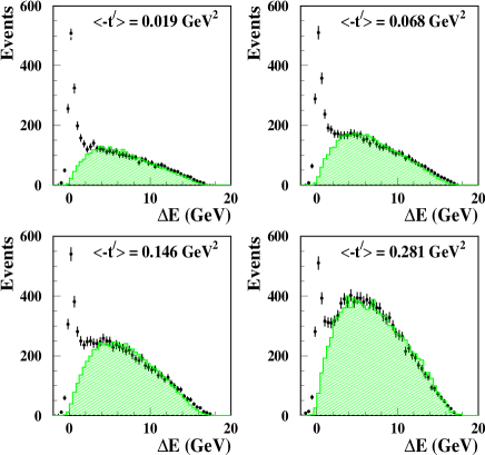
The amount of SIDIS background and its angular distributions in the exclusive region can not be determined with the present apparatus. Therefore, the PYTHIA code sjo03 tuned for HERMES kinematic conditions lieb04 ; vanm05 ; ulie06 is used. Exclusive processes were excluded from the simulated sample. The simulated SIDIS events were passed through the same chain of kinematic requirements as the experimental ones. Very good agreement between the experimental data and the simulation is observed for the shape of the $\Delta E$ distributions in the region $\Delta E>2$ GeV for each kinematic interval in $Q^{2}$, $x$ or $t^{\prime}$, and for both targets. This agreement in shape is demonstrated in Fig. 6, which shows four intervals in $t^{\prime}$ as an example. Since no absolute normalization between data and simulation is required to determine the SDMEs (as shown in the next section), for every kinematic interval the fractional background contribution $f_{bg}$ in the exclusive region can be obtained by normalizing the simulation to the data in the region $2~{}{\rm GeV}<\Delta E<20$ GeV. That is,

$$f_{bg}=(N_{excl}^{MC}/N_{excl}^{data})\;(N_{2-20}^{data}/N_{2-20}^{MC}),$$ (44)

where $N^{data}_{2-20}$, $N^{MC}_{2-20}$ and $N^{data}_{excl}$, $N^{MC}_{excl}$ are the total number of measured and simulated events at $2~{}{\rm GeV}<\Delta E<20$ GeV and in the exclusive region, respectively. This contribution amounts to 8% for the entire kinematic region and ranges between 3 and 12% in the different kinematic intervals. These values will be used for the subtraction of the SIDIS background angular distributions, as described in section 6.2.

b) Background from Non-resonant Exclusive $\pi^{+}\pi^{-}$ Pairs

The contribution of non-resonant $\pi^{+}\pi^{-}$ production and its interference soeding with resonant $\rho^{0}\to\pi^{+}$ $\pi^{-}$ production are determined using a modified Breit-Wigner fit to the invariant mass distribution. We do not distinguish between resonant and non-resonant contributions in $\rho^{0}$ production, following the practice of previous experimental zeussdme ; compasssdme and theoretical publications ryskin ; manaenkov ; golos ; golos2 . Therefore the present data were not corrected for non-resonant background, which amounts to $\sim 4$ – $8$% depending on the kinematics rho-xsec ; dsa-lipka ; tytgat . Note that the contribution of $\rho^{0}$-$\omega$ interference has been found to be negligible rho-xsec .

c) Background from Proton-Dissociative Processes

Another possible background consists of events in which the target proton is excited to some other baryonic resonance, which then decays to a proton and typically a soft pion. In the absence of a recoil detector, such events cannot be distinguished, but their contribution to the exclusive $\rho^{0}$ production cross section at HERMES was found to be small ($4\pm 2\%$) rho-xsec . No correction has been applied for this background, as the extracted SDMEs were found to change negligibly at a value of $\Delta E$=0.2 GeV, where this background is strongly suppressed. This approach is supported by results from ZEUS, where the decay angle distributions of the proton-dissociative reaction have been found to be consistent with those of exclusive events zeussdme ; zeussdme2 .

6 Extraction of SDMEs

6.1 Maximum Likelihood Method

In each bin of $Q^{2}$ or $t^{\prime}$, or the entire acceptance, the SDMEs are obtained by minimizing the difference between the 3-dimensional $(\cos\Theta,\phi,\Phi)$ production and decay angle distribution of the experimental events and that of a sample of fully reconstructed Monte Carlo events, using a binned maximum likelihood method. For the Monte Carlo simulation, events are generated isotropically in ($\Phi,\phi,\cos\Theta$) using the rhoMC generator rho-xsec ; sdme-publ ; craig for exclusive $\rho^{0}$ production, simulated in the instrumental context of the spectrometer, and passed through the same reconstruction chain as the experimental data. Introduction of estimated misalignments of the spectrometer into the Monte Carlo simulation used for the SDME extraction was found to have a negligible effect on the results. The variables $\cos\Theta$, $\phi$, and $\Phi$ are binned in $8\times 8\times 8$ cells. The content of each of the 512 cells is weighted using (37), whereby the 23 matrix elements are treated as free parameters. The number of events $d_{i}$ in each cell is assumed to obey a Poisson distribution:

$$P(d_{i},c_{N}m^{\prime}_{i})=\frac{(c_{N}m^{\prime}_{i})^{d_{i}}}{d_{i}!}e^{-c_{N}m^{\prime}_{i}},$$ (45)

with mean value $c_{N}m^{\prime}_{i}$, where $c_{N}=(\sum_{j}d_{j})/(\sum_{j}m^{\prime}_{j})$ is a normalization factor accounting for the difference in the total number of events in the data ($d_{j}$) and simulated ($m^{\prime}_{j}$) sample, and $m^{\prime}_{i}$ is the (re)weighted number of simulated events in cell $i$. The likelihood function is then defined as zech

$$L(\lambda)=\prod_{i}^{cells}P\left(d_{i},c_{N}(\lambda)m^{\prime}_{i}(\lambda)\right),$$ (46)

where $\lambda$ represents the 23 fit parameters that are the 23 SMDEs. The best fit parameters were determined by maximizing the logarithm of the likelihood function,

$$\ln L(\lambda) = \sum_{i}\left[d_{i}\ln\left(c_{N}(\lambda)m^{\prime}_{i}(\lambda)\right)-c_{N}(\lambda)m^{\prime}_{i}\right]$$ (47)

$$\hskip 21.33955pt+{\it\ constant},$$

or equivalently by minimizing $-\ln L(\lambda)$.

The minimization itself and the uncertainty calculation are performed using the MINUIT package minuit . In the fitting procedure the samples with negative and positive beam helicity are fitted simultaneously. The values of $\chi^{2}$ per degree of freedom ($\chi^{2}/d.o.f.$) for the 16 kinematic intervals ($Q^{2}$, $t^{\prime}$ or $x$), calculated after completing their likelihood fits, range between 0.6 and 1.2 for $8\times 8\times 8-23$ degrees of freedom. For every SDME, the averages of the SDMEs extracted from the two separate beam helicity samples are found to be consistent with each other and the result from the common fit.

In Fig. 7 one-dimensional angular distributions are shown for the hydrogen and deuterium data samples, where the positive-helicity sample is chosen as representative. In addition to distributions in $\cos\Theta$, $\phi$, and $\Phi$, the angular distribution in $\psi=\phi-\Phi$ is shown, which embodies the entire azimuthal dependence in the case of SCHC. For each panel, the data are compared with the isotropic input distributions as modified by instrumental effects such as acceptance, tracking resolution, and reconstruction efficiencies, as well as the one-dimensional projections of the fitted 3-dimensional angular distribution. These projections are clearly in agreement with the data.

Figure 7: Angular distributions with common arbitrary normalization for $\rho^{0}$ meson production and decay. Data points represent the positive helicity sample of the proton (deuteron) data in the left (right) half of the figure. The dotted lines represent isotropic input Monte Carlo distributions as modified by the HERMES acceptance, while the dashed lines are the results of the 23-parameter fit. Here 16 bins are chosen for a more detailed comparison. The data correspond to the full kinematic region of the analysis.

6.2 Background Subtraction

Before fitting SDMEs to the ($\cos\Theta,\phi,\Phi$) angular distributions, the SIDIS background in the exclusive region is subtracted. This subtraction is performed separately for each interval in $t^{\prime}$, $Q^{2}$ or $x$. In a given ($\cos\Theta,\phi,\Phi$) cell, the number of background events in the exclusive region is calculated as follows:

$$N^{bg}_{cell}=N^{MC}_{cell}\;\frac{N^{data}_{2-20}}{N^{MC}_{2-20}},$$ (48)

where the number of SIDIS Monte Carlo events in a given cell is $N^{MC}_{cell}$, while $N^{data}_{2-20}$ and $N^{MC}_{2-20}$ are defined as in equation (44).

6.3 Systematic Uncertainties

a) Background Subtraction

The systematic uncertainty of the background subtraction procedure is estimated as the difference between the SDMEs obtained with and without any background correction.

b) rhoMC Input Parameters

The SDME extraction procedure starts from isotropic distributions in $\cos\Theta$, $\phi$, and $\Phi$ generated by rhoMC, as explained above. The parameterization of the total electroproduction cross section in rhoMC is chosen in the context of a VMD model that incorporates a propagator-type $Q^{2}$ dependence, and also contains a dependence on $R(Q^{2})$. As the HERMES spectrometer acceptance depends on $Q^{2}$, different input parameters result in slightly different reconstructed angular distributions. The corresponding systematic uncertainty of the resulting SDMEs is obtained by varying these parameters within one standard deviation in the total uncertainty of the parameters given in Refs. rho-xsec ; sdme-publ .

The total systematic uncertainty is obtained by adding in quadrature the uncertainty from the background subtraction procedure and that due to the uncertainty in the rhoMC input parameters, which are approximately of equal size.

c) Further Systematic Studies

Several further studies using generated and reconstructed event samples are performed to estimate possible systematic uncertainties:

i) A consistency check of the extraction method is performed by using several known sets of SDMEs as input to the rhoMC rho-xsec ; sdme-publ ; craig simulation and comparing the SDMEs extracted from the simulated data with those used as input to the rhoMC generator. First, isotropic angular distributions were simulated, corresponding to all SDMEs vanishing except $r^{04}_{00}=\frac{1}{3}$. Alternatively, events were generated assuming SCHC, implying that only five unpolarized and two polarized SDMEs are non-zero, as explained in section 3.7. Finally, the extracted 23 SDMEs are used as input parameters. In all cases, good agreement is found between input and extracted SDMEs at the given level of statistical accuracy.

ii) Several tests are performed to ensure that the choice of the ($\cos\Theta,\phi,\Phi$) cell size does not bias the results of the maximum likelihood procedure. A sample of about 40000 simulated events with angular dependences determined by the (normally) extracted 23 SDMEs is fitted after binning the data in several numbers of angular cells, varying from $5\times 5\times 5$ to $12\times 12\times 12$. The $\chi^{2}/d.o.f.$ calculated between sets of SDMEs extracted with $8\times 8\times 8$ and $12\times 12\times 12$ binning is $0.14$. Hence the cell size used in the maximum likelihood procedure is not treated as a source of systematic uncertainty.

iii) Variations of the restrictions on $M_{\pi^{+}\pi^{-}}$, $t^{\prime}$, and $\Delta E$ result in slightly different amounts of SIDIS background. The resulting systematic uncertainty is much smaller than that estimated for the background subtraction procedure, and hence is neglected.

iv) In the SDME extraction procedure, only the shape of the 3-dimensional angular distribution matters. As events in which a radiative photon is emitted with an energy larger than 0.6 GeV are removed from the analysis by the constraint $\Delta E<0.6$ GeV, the impact of radiative effects on the shape of the 3-dimensional angular distribution is strongly reduced. Two approaches are used to quantify this effect. First, the DIFFRAD code is used to calculate the radiative effects for exclusive $\rho^{0}$ production akush ; akush2 , as was done also in Refs. zeussdme ; tytgat . As the emission of a real photon by the positron alters the direction of the virtual photon, the angle $\Phi$ between lepton scattering plane and $\rho^{0}$ production plane also changes. The effect of a small variation ($<2.5$ %, as suggested in Ref. akush2 ) of the shape of the $\Phi$-distribution is studied by re-weighting the isotropic input angular distribution. The difference between SDMEs obtained with and without re-weighting is found to be less than 0.0012 for all SDMEs ($\chi^{2}/d.o.f.<0.1$), i.e., radiative effects are negligible.

As an independent cross check, radiative effects on the extracted SDMEs are studied using a Monte Carlo simulation of exclusive $\rho^{0}$ production with events from the PYTHIA generator sjo03 . Two statistically independent isotropic angular distributions are generated, with and without the emission of radiative photons. A set of SDMEs is extracted from the (real) data sample for each of these isotropic input angular distributions. The difference between the resulting SDMEs is statistically indistinguishable ($\chi^{2}/d.o.f.\leq 0.2$).

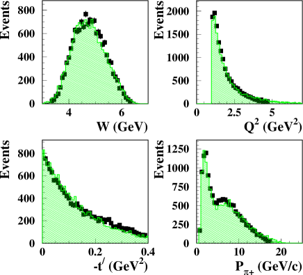
As a further check we use the extracted 23 SDMEs as input parameters to rhoMC and compare the shapes of the simulated distributions with the data. In order to restrict the comparison to exclusive $\rho^{0}$ events, properly normalized SIDIS background distributions from PYTHIA are subtracted from the data. In the maximum likelihood fit method, the extraction of SDMEs only requires simulated event distributions normalized to the data. The shape comparison reveals good agreement for all variables, some of which are presented in Fig. 8.

Figure 8: Shape comparison of the distributions in $W$, $Q^{2}$, $t^{\prime}$ and $P_{\pi^{+}}$, the momentum of the $\pi^{+}$ from $\rho^{0}$ decay in the laboratory system, for the hydrogen data sample (squares). The shaded areas show rhoMC results using the extracted 23 SDMEs as input for the simulation, normalized to the data. Background has been subtracted from the data.

7 Results on SDMEs Integrated over the Entire Kinematic Region

7.1 Classification of SDMEs

The presentation of the extracted SDMEs will be based on a hierarchy of NPE helicity amplitudes:

$$|T_{00}|\sim|T_{11}|\gg|T_{01}|>|T_{10}|\gtrsim|T_{1-1}|.$$ (49)

A similar hierarchy was discussed for the first time in Ref. divanov . In perturbative QCD this is valid at asymptotically high $Q^{2}$. It was experimentally confirmed at the HERA collider zeussdme ; zeussdme2 ; H1 and discussed in Refs. ipivanov ; manaenkov ; golos . In the following it will be shown that it applies also at $Q^{2}$ values typical of the HERMES experiment.

The extracted 23 SDMEs are categorized into five classes according to the hierarchy shown above. Class A comprises SDMEs dominated by the helicity-conserving amplitudes $T_{00}$ and $T_{11}$ which describe the transitions $\gamma^{*}_{L}\to\rho^{0}_{L}$ and $\gamma^{*}_{T}\to\rho^{0}_{T}$, respectively. Class B contains SDMEs that correspond to the interference of the above two amplitudes. Class C consists of all those SDMEs in which the main term contains a contribution linear in the $s$-channel helicity non-conserving amplitude $T_{01}$, corresponding to the $\gamma^{*}_{T}\to\rho^{0}_{L}$ transition, except for a term involving $r^{1}_{00}$ for which the $T_{01}$ contribution is quadratic. The classes D and E are composed of the SDMEs in which the main terms contain a contribution linear in the small helicity-flip amplitudes $T_{10}$ ($\gamma^{*}_{L}\to\rho^{0}_{T}$) and $T_{1-1}$ ($\gamma^{*}_{-T}\to\rho^{0}_{T}$), respectively. Equations (77-99) in Appendix A show the representation of all the SDMEs in terms of helicity amplitudes ordered according to the five classes defined above.

7.2 Representation of the Integrated Data

Separate maximum likelihood fits to the proton and deuteron data samples are performed in the entire kinematic region: $1~{}{\rm GeV}^{2}<Q^{2}<7$ GeV², $3~{}{\rm GeV}<W<6.3$ GeV (corresponding to $0.03<x_{B}<0.25$), and $0~{}{\rm GeV}^{2}<-t^{\prime}<0.4$ GeV². The resulting $\rho^{0}$ meson SDMEs $r^{\alpha}_{\lambda_{V}\lambda^{\prime}_{V}}$ are listed in Tab. 1 and displayed in Fig. 9, ordered according to the classes described above. The statistical uncertainties are larger for the eight polarized SDMEs (shown in the shaded areas of the figure) due to the non-unity of the beam polarization and the kinematic suppression factor $\sqrt{1-\epsilon}$ (see (39)). In order to facilitate comparison with a recently introduced new representation of SDMEs mdiehl , the proton SDMEs in that representation are shown in Tab. 14 of Appendix E.

Table 1: Values of $\rho^{0}$ SDMEs for proton and deuteron data ordered in classes by horizontal lines according to the expected hierarchy of helicity amplitudes. Elements $r^{\alpha}_{ij}$ with $\alpha=3,7,8$ are polarized. The first uncertainty is statistical, the second systematic. The statistical significance of the magnitude of each SDME expected to vanish in the case of SCHC is shown in column three or five as its absolute value in units of standard deviations of its total uncertainty, denoted as SDME/$tot$. Similarly, the four bottom rows of the table show deviations from zero of certain combinations of SDMEs that would thereby violate SCHC and NPE dominance (see text).

	proton		deuteron
element	SDME $\pm stat\pm syst$	SDME/$tot$	SDME $\pm stat\pm syst$	SDME/$tot$
$r^{04}_{00}$	0.412 $\pm$ 0.010 $\pm$ 0.010		0.416 $\pm$ 0.007 $\pm$ 0.013
$r^{1}_{1-1}$	0.246 $\pm$ 0.011 $\pm$ 0.019		0.247 $\pm$ 0.008 $\pm$ 0.014
Im $r^{2}_{1-1}$	$-0.227$ $\pm$ 0.010 $\pm$ 0.012		$-0.234$ $\pm$ 0.008 $\pm$ 0.019
Re $r^{5}_{10}$	0.161 $\pm$ 0.004 $\pm$ 0.010		0.165 $\pm$ 0.003 $\pm$ 0.010
Im $r^{6}_{10}$	$-0.167$ $\pm$ 0.003 $\pm$ 0.009		$-0.156$ $\pm$ 0.003 $\pm$ 0.006
Im $r^{7}_{10}$	0.112 $\pm$ 0.021 $\pm$ 0.011		0.104 $\pm$ 0.016 $\pm$ 0.004
Re $r^{8}_{10}$	0.074 $\pm$ 0.019 $\pm$ 0.006		0.114 $\pm$ 0.014 $\pm$ 0.009
Re $r^{04}_{10}$	0.031 $\pm$ 0.004 $\pm$ 0.008	3.5	0.030 $\pm$ 0.003 $\pm$ 0.008	3.5
Re $r^{1}_{10}$	$-0.032$ $\pm$ 0.007 $\pm$ 0.012	2.3	$-0.020$ $\pm$ 0.006 $\pm$ 0.010	1.7
Im $r^{2}_{10}$	0.022 $\pm$ 0.007 $\pm$ 0.015	1.3	0.014 $\pm$ 0.006 $\pm$ 0.017	0.8
$r^{5}_{00}$	0.109 $\pm$ 0.009 $\pm$ 0.009	8.7	0.111 $\pm$ 0.007 $\pm$ 0.008	10.4
$r^{1}_{00}$	0.011 $\pm$ 0.019 $\pm$ 0.008	0.6	$-0.038$ $\pm$ 0.015 $\pm$ 0.016	1.7
Im $r^{3}_{10}$	$-0.017$ $\pm$ 0.015 $\pm$ 0.004	1.1	0.031 $\pm$ 0.011 $\pm$ 0.003	2.7
$r^{8}_{00}$	0.035 $\pm$ 0.050 $\pm$ 0.010	0.7	0.053 $\pm$ 0.038 $\pm$ 0.006	1.4
$r^{5}_{11}$	$-0.01$ $\pm$ 0.003 $\pm$ 0.013	1.2	$-0.021$ $\pm$ 0.003 $\pm$ 0.013	1.6
$r^{5}_{1-1}$	0.005 $\pm$ 0.004 $\pm$ 0.006	0.7	0.013 $\pm$ 0.003 $\pm$ 0.006	1.9
Im $r^{6}_{1-1}$	$-0.002$ $\pm$ 0.004 $\pm$ 0.007	0.3	$-0.007$ $\pm$ 0.003 $\pm$ 0.006	1.0
Im $r^{7}_{1-1}$	$-0.035$ $\pm$ 0.030 $\pm$ 0.005	1.2	$-0.058$ $\pm$ 0.023 $\pm$ 0.009	2.3
$r^{8}_{11}$	0.036 $\pm$ 0.024 $\pm$ 0.001	1.6	0.026 $\pm$ 0.018 $\pm$ 0.003	1.4
$r^{8}_{1-1}$	0.019 $\pm$ 0.029 $\pm$ 0.005	0.6	$-0.066$ $\pm$ 0.022 $\pm$ 0.008	2.8
$r^{04}_{1-1}$	$-0.011$ $\pm$ 0.005 $\pm$ 0.005	1.5	$-0.002$ $\pm$ 0.004 $\pm$ 0.008	0.2
$r^{1}_{11}$	$-0.025$ $\pm$ 0.007 $\pm$ 0.008	2.3	$-0.002$ $\pm$ 0.006 $\pm$ 0.013	0.1
Im $r^{3}_{1-1}$	$-0.024$ $\pm$ 0.018 $\pm$ 0.001	1.3	$-0.004$ $\pm$ 0.014 $\pm$ 0.004	0.3
relation	SCHC?		SCHC?
$r^{1}_{1-1}$ + Im $r^{2}_{1-1}$	0.018 $\pm$ 0.012 $\pm$ 0.011	1.1	0.013 $\pm$ 0.009 $\pm$ 0.014	0.8
Re $r^{5}_{10}+$ Im $r^{6}_{10}$	$-0.006$ $\pm$ 0.004 $\pm$ 0.001	1.5	0.010 $\pm$ 0.003 $\pm$ 0.005	1.7
Im $r^{7}_{10}-$ Re $r^{8}_{10}$	0.038 $\pm$ 0.029 $\pm$ 0.006	1.3	$-0.011$ $\pm$ 0.022 $\pm$ 0.006	0.5
relation	SCHC and NPE?		SCHC and NPE?
$1-r^{04}_{00}-2r^{1}_{1-1}$	0.097 $\pm$ 0.017 $\pm$ 0.046	2.0	0.091 $\pm$ 0.013 $\pm$ 0.038	2.3

Figure 9: The 23 SDMEs extracted from $\rho^{0}$ data: proton (squares) and deuteron (circles) in the entire HERMES kinematics with $\langle x\rangle=0.08,\langle Q^{2}\rangle=1.95$ GeV², $\langle-t^{\prime}\rangle=0.13$ GeV². The SDMEs are multiplied by prefactors in order to represent the normalized leading contribution of the corresponding amplitude (see (77-99)). The inner error bars represent the statistical uncertainties, while the outer ones indicate the statistical and systematic uncertainties added in quadrature. SDMEs measured with unpolarized (polarized) beam are displayed in the unshaded (shaded) areas. The vertical dashed line at zero is indicated for SDMEs expected to be zero under the hypothesis of SCHC.

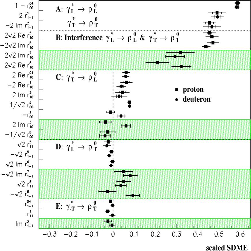
In Fig. 9 the SDMEs are shown multiplied by certain factors in order to allow their comparison at the level of dominant amplitudes (see (77-99)). For all classes numerical factors are chosen in such a way that the coefficient of the dominant terms is equal to unity. The plotted representatives for the elements of class A are chosen so that their main terms are equal to $|T_{11}|^{2}/\mathcal{N}$; in particular this requires that the term $1-r^{04}_{00}$ be chosen. The coefficients for class B are chosen to have the main contribution to the plotted representatives for the unpolarized and polarized SDMEs equal to $\mathrm{Re}\{T_{11}T^{*}_{00}\}/\mathcal{N}$ and $\mathrm{Im}\{T_{11}T^{*}_{00}\}/\mathcal{N}$, respectively. This corresponds to the general rule that is applicable to classes B to E: the dominant contribution of the unpolarized (polarized) element presented in Fig. 9 is proportional to the real (imaginary) part of a product of two amplitudes. Class C contains the main terms $T_{01}T^{*}_{00}/\mathcal{N}$ (for $r^{5}_{00}/\sqrt{2}$ and $r^{8}_{00}/\sqrt{2}$) and $T_{01}T^{*}_{11}/\mathcal{N}$. The dominant contributions for classes D and E contain terms $T_{10}T^{*}_{11}/\mathcal{N}$ and $T_{1-1}T^{*}_{11}/\mathcal{N}$, respectively.

Given the scaled SDMEs in Fig. 9, it easily can be seen that the two unpolarized SDMEs of class B have large values, similar to those of class A. This suggests the presence of a substantial interference between the two dominant amplitudes $T_{00}$ and $T_{11}$. The two polarized class B SDMEs are significantly non-zero for proton and deuteron as well. It is also seen that the values of elements in class C that contain the dominant term $T_{01}T^{*}_{11}$ are similar for the unpolarized SDMEs ($\mathrm{Re}\{r^{04}_{10}\}$, $\mathrm{Re}\{r^{1}_{10}\}$, $\mathrm{Im}\{r^{2}_{10}\}$). Those unpolarized class C elements measured with good accuracy, $\mathrm{Re}\{r^{04}_{10}\}$ and $r^{5}_{00}$, are much smaller than the class B SDMEs, whereas the unpolarized class C elements are larger than the unpolarized class D and class E SDMEs. This shows that the anticipated hierarchy is supported by the data. For class D SDMEs, slightly positive (negative) values are observed in the polarized (unpolarized) case. Finally, values of class E SDMEs for the proton target tend to deviate from zero, while those for the deuteron ones are consistent with zero.

We note that no significant difference is found between the sets of SDMEs for proton and deuteron, as a $\chi^{2}/d.o.f.=22.5/23$ is obtained taking into account the total uncertainties. Hence there appears to be no indication of significant contributions of secondary reggeons with isospin $I=1$ and natural parity.

7.3 Test of the SCHC Hypothesis

As explained in section 3.7, only the following seven SDMEs are not restricted to be zero in the case of $s$-channel helicity conservation: $r^{04}_{00}$, $r^{1}_{1-1}$, Im$\{r^{2}_{1-1}\}$, Re$\{r^{5}_{10}\}$, Im$\{r^{6}_{10}\}$ and Im$\{r^{7}_{10}\}$, Re$\{r^{8}_{10}\}$. All other SDMEs are required by SCHC to be zero. The magnitudes of their measured offsets from zero, expressed in units of the standard deviation of their uncertainty, are shown in one of two separate columns of Tab. 1, next to the respective SDME. Several elements are inconsistent with the hypothesis of SCHC, in particular several members of class C.

The SDME $r^{5}_{00}$ is observed to be non-zero at the level of nine (ten) standard deviations in the total uncertainty for the proton (deuteron) result, proving $s$-channel helicity non-conservation. This was already observed earlier by the HERA collider experiments zeussdme ; H1 at a lower significance level, and with high significance very recently zeussdme2 . For the first time, HERMES observes $s$-channel helicity non-conservation also in other class C SDMEs, in particular $\mathrm{Re}\{r^{04}_{10}\}$.

The polarized elements $r^{8}_{00}$ and $\mathrm{Im}\{r^{3}_{10}\}$, related to the terms Im$\{T_{01}T_{00}^{*}\}$ and Im$\{T_{01}T_{11}^{*}\}$ respectively (89,90), are extracted using a longitudinally polarized lepton beam for the first time. Both elements are consistent with zero (Figs. 9, 13) within the uncertainties.

The relations imposed by the hypothesis of SCHC (40-42) are satisfied within about one standard deviation of the total uncertainty, as can be seen from the corresponding rows of Tab. 1. The sensitivity of these relations to SCHC is low. In the case of the relation (40) only the contributions of small double-helicity-flip amplitudes (see (78,79) ) violate SCHC. For the relations (41-42), equations (80-83) show that the largest SCHC amplitude $T_{00}$ is multiplied by the smallest $T_{1-1}$ amplitude in the terms that violate SCHC. The relation corresponding to the combined hypotheses of SCHC and NPE dominance (43) is marginally violated by two standard deviations in the total uncertainty. In evaluating the uncertainties of these relations, correlations between the corresponding elements (see Tabs. 15,16), are taken into account.

7.4 Phase Difference between $\mathbf{T_{11}}$ and $\mathbf{T_{00}}$

The phase difference $\delta$ between the amplitudes $T_{11}$ and $T_{00}$ can be evaluated as follows:

$$\cos\delta=\frac{2\sqrt{\epsilon}(\mathrm{Re}\{r^{5}_{10}\}-\mathrm{Im}\{r^{6}_{10}\})}{\sqrt{r^{04}_{00}(1-r^{04}_{00}+r^{1}_{1-1}-\mathrm{Im}\{r^{2}_{1-1}\})}}.$$ (50)

This results in $|\delta|=26.4\pm 2.3_{stat}\pm 4.9_{syst}$ degrees for the proton and $|\delta|=29.3\pm 1.6_{stat}\pm 3.6_{syst}$ degrees for the deuteron (see Fig. 12). Using polarized SDMEs, also the sign of $\delta$ can be determined:

$$\sin\delta=\frac{2\sqrt{\epsilon}(\mathrm{Re}\{r^{8}_{10}\}+\mathrm{Im}\{r^{7}_{10}\})}{\sqrt{r^{04}_{00}(1-r^{04}_{00}+r^{1}_{1-1}-\mathrm{Im}\{r^{2}_{1-1}\})}}.$$ (51)

Equations (50) and (51) are derived in Appendix B. Second order contributions of spin-flip amplitudes are neglected in obtaining these formulae.

Using (51) it is determined, for the first time, that the sign of $\delta$ is positive: $\delta=30.6\pm 5.0_{stat}\pm 2.4_{syst}$ degrees for the proton and $\delta=36.3\pm 3.9_{stat}\pm 1.7_{syst}$ for the deuteron. These values are consistent with each other and their magnitudes are in agreement with the results obtained with (50) for $\cos{\delta}$.

We note that in the GPD-based model of Ref. golos3 , the phase difference between the amplitudes $T_{11}$ and $T_{00}$ is found to have a value of about 3 degrees. This appears to be inconsistent with the HERMES results and also, to a lesser extent, with the H1 results H1 ; the two experimental results agree within their total uncertainties.

Figure 10: $Q^{2}$ and $t^{\prime}$ dependences of class A SDMEs describing the dominant transitions $\gamma^{*}_{L}\to\rho^{0}_{L}$ and $\gamma^{*}_{T}\to\rho^{0}_{T}$. Filled squares (circles) correspond to proton (deuteron) data. Total uncertainties are depicted, calculated as statistical and systematic uncertainties combined in quadrature. Deuterium data points are presented with a small horizontal offset here and in Figs. (11-18) to improve their visibility.

Figure 11: $Q^{2}$ and $t^{\prime}$ dependences of the class B SDMEs describing the interference of the dominant transitions $\gamma^{*}_{L}\to\rho^{0}_{L}$ and $\gamma^{*}_{T}\to\rho^{0}_{T}$. Filled squares (circles) correspond to proton (deuteron) data. Total uncertainties are depicted, calculated as statistical and systematic uncertainties combined in quadrature.

Figure 12: The $Q^{2}$ dependence of the phase difference $\delta$ between $T_{11}$ and $T_{00}$ amplitudes calculated according to (50) for the proton (filled squares) and deuteron (filled circles) data. The values of $\delta$, for yields integrated over the range $1~{}{\rm GeV}^{2}<Q^{2}<7$ GeV², are shown as open symbols. The inner (outer) bars represent the statistical (total) uncertainty.

8 The $\mathbf{Q^{2}}$ and $\mathbf{t^{\prime}}$ Dependences of the SDMEs

In the following, the $Q^{2}$ dependences are presented in four bins, where the first bin is defined by $0.5~{}{\rm GeV}^{2}<Q^{2}<1$ GeV² with $\langle Q^{2}\rangle=0.83$ GeV². For the $t^{\prime}$ dependences, also shown in four bins, only data with $Q^{2}>1$ GeV² are included. The average value of $t^{\prime}$ is almost independent of $Q^{2}$ and $W$.

8.1 Class A: Dominant Transitions $\mathbf{\gamma^{*}_{L}\to\rho^{0}_{L}}$ and $\mathbf{\gamma^{*}_{T}\to\rho^{0}_{T}}$

Class A comprises SDMEs corresponding to the dominant transitions, $\gamma^{*}_{T}\rightarrow\rho^{0}_{T}$ and $\gamma^{*}_{L}\rightarrow\rho^{0}_{L}$, described by the amplitudes $T_{11}$ and $T_{00}$. The $Q^{2}$ and $t^{\prime}$ dependences for the class A SDMEs $1-r^{04}_{00}$, $r^{1}_{1-1}$, and $\mathrm{Im}\{r^{2}_{1-1}\}$ are shown in Fig. 11. The three elements exhibit somewhat similar $Q^{2}$ dependences. They are found to be approximately constant over the measured $t^{\prime}$ range, as also observed by ZEUS zeussdme2 for $r^{04}_{00}$ at average $Q^{2}$ values of 3 and 10 GeV². Such a $t^{\prime}$ independence indicates similar $t^{\prime}$-slopes for longitudinal and transverse components of the vector meson production cross section.

We note that there is good agreement between the highest $Q^{2}$ points of the HERMES proton data and the GPD-based model calculations of Ref. golos3 .

8.2 Class B: Interference of $\mathbf{\gamma^{*}_{L}\to\rho^{0}_{L}}$ and $\mathbf{\gamma^{*}_{T}\to\rho^{0}_{T}}$ Transitions

Class B comprises SDMEs describing the interference of the dominant transitions $\gamma^{*}_{T}\rightarrow\rho^{0}_{T}$ and $\gamma^{*}_{L}\rightarrow\rho^{0}_{L}$, i.e., those corresponding to a product of the amplitude $T_{11}$ and the complex conjugate of $T_{00}$. Polarized (unpolarized) SDMEs correspond to the real (imaginary) part of this product.

Figure 11 shows the $Q^{2}$ and $t^{\prime}$ dependence of these SDMEs. It is apparent that the SCHC relations (41) and (42) are approximately fulfilled over the measured kinematic ranges. Considering (80-83), this implies that contributions of single- and double-helicity-flip amplitudes are small.

An indication of a $Q^{2}$ dependence of the phase difference $\delta$ between the amplitudes $T_{11}$ and $T_{00}$ (see (50)) is presented in Fig. 12. The result of a fit with a linear $Q^{2}$ dependence has a $\chi^{2}/d.o.f.=$ 1.41/2 (1.42/2) for the proton (deuteron) data, which is smaller than the fit result with no $Q^{2}$ dependence: $\chi^{2}/d.o.f.=$ 4.52/3 (4.38/3). Note that at the lowest $Q^{2}$, the value of $\delta$ has the largest systematic uncertainty due to the rapidly falling acceptance of the HERMES spectrometer. No $t^{\prime}$ dependence of $\delta$ is observed, for either target.

Figure 13: $Q^{2}$ and $t^{\prime}$ dependence of the class C SDMEs describing the interference of the helicity-flip transition $\gamma^{*}_{T}\to\rho^{0}_{L}$ and one of the dominant helicity-conserving transition. Filled squares (circles) correspond to proton (deuteron) data. Total uncertainties are depicted, calculated as statistical and systematic uncertainties combined in quadrature.

Figure 14: $Q^{2}$ and $t^{\prime}$ dependences of class D SDMEs describing the interference of the helicity-flip transition $\gamma^{*}_{L}\to\rho^{0}_{T}$ and the dominant transition $\gamma^{*}_{T}\to\rho^{0}_{T}$. Filled squares (circles) correspond to proton (deuteron) data. Total uncertainties are depicted, calculated as statistical and systematic uncertainties combined in quadrature.

Figure 15: $Q^{2}$ and $t^{\prime}$ dependences of the class E SDMEs describing the interference of the double-helicity-flip transition $\gamma^{*}_{-T}\to\rho^{0}_{T}$ and the dominant transition $\gamma^{*}_{T}\to\rho^{0}_{T}$. Filled squares (circles) correspond to proton (deuteron) data. Total uncertainties are depicted, calculated as statistical and systematic uncertainties combined in quadrature.

8.3 Class C: Helicity-Flip Transition $\mathbf{\gamma^{*}_{T}\to\rho^{0}_{L}}$

Class C consists of all those SDMEs with the main term containing a product of the s-channel helicity violating amplitude $T_{01}$ describing the helicity-flip transition $\gamma^{*}_{T}\to\rho^{0}_{L}$, and the complex conjugate of $T_{00}$, $T_{11}$ or $T_{01}$, (see (84-90)). No clear $Q^{2}$ dependence is observed for class C SDMEs (see Fig. 13).

As suggested by general properties of helicity-flip kinematics at low $t^{\prime}$ values, a dependence on $\sqrt{-t^{\prime}}$ that monotonically increases from zero is expected for the amplitude $T_{01}$ mdiehl . This is consistent with the measured SDMEs containing this amplitude, as is clearly seen for $r^{5}_{00}$ and $\mathrm{Re}\{r^{04}_{10}\}$ in the third row of Fig. 13.

8.4 Class D: Helicity-Flip Transition $\mathbf{\gamma^{*}_{L}\to\rho^{0}_{T}}$

Class D consists of SDMEs for which the main terms in (91-96) contain a product of the small helicity-flip amplitude $T_{10}$ with the complex conjugate of $T_{11}$. Unpolarized (polarized) SDMEs represent the real (imaginary) part of this product. Correspondingly, they describe the interference of the helicity-flip transition $\gamma^{*}_{L}\rightarrow\rho^{0}_{T}$ with the helicity-conserving transition $\gamma^{*}_{T}\rightarrow\rho^{0}_{T}$. Figure 14 shows that the class D SDMEs depends only weakly on $Q^{2}$ and $t^{\prime}$, and are consistent with zero as $-t^{\prime}\to 0$, as expected.

8.5 Class E: Double Helicity-Flip Transition $\mathbf{\gamma^{*}_{-T}\to\rho^{0}_{T}}$

Class E consists of the SDMEs with the main term describing the interference of the transition $\gamma^{*}_{-T}\rightarrow\rho^{0}_{T}$ with $\gamma^{*}_{T}\rightarrow\rho^{0}_{T}$. This corresponds to a product of the double spin-flip amplitude $T_{1-1}$ with the complex conjugate of the helicity-conserving amplitude $T_{11}$. Unpolarized (polarized) SDMEs represent the real (imaginary) part of this product. Their $Q^{2}$ and $t^{\prime}$ dependences are presented in Fig. 15, where it can be seen that the class D SDMEs depend only weakly on $Q^{2}$ and $t^{\prime}$, and are consistent with zero as $-t^{\prime}\to 0$, as expected.

9 Unnatural-Parity Exchange

For $\rho^{0}$ production on the proton, or incoherent production on the deuteron, the existence of unnatural-parity exchange can be tested by evaluating the following combinations of SDMEs:

$$u_{1}=1-r_{00}^{04}+2r_{1-1}^{04}-2r_{11}^{1}-2r_{1-1}^{1},$$ (52)

$$u_{2}=r^{5}_{11}+r^{5}_{1-1},$$ (53)

$$u_{3}=r^{8}_{11}+r^{8}_{1-1}.$$ (54)

If UPE is absent, all three combinations are expected to vanish without resort to SCHC. A non-zero result for

$$u_{1}=\widetilde{\sum}\{4\epsilon|U_{10}|^{2}+2|U_{11}+U_{-11}|^{2}\}/\mathcal{N}$$ (55)

indicates the existence of UPE contributions, while the value for

$$u_{2}+iu_{3}=\sqrt{2}\;\widetilde{\sum}\{(U_{11}+U_{-11})^{*}U_{10}\}/\mathcal{N}$$ (56)

can vanish despite the existence of UPE contributions. Such a behavior can be explained if a hierarchy exists also for unnatural-parity-exchange amplitudes:

$$\widetilde{\sum}|U_{11}|^{2}\gg\widetilde{\sum}|U_{10}|^{2},\widetilde{\sum}|U_{01}|^{2},\widetilde{\sum}|U_{-11}|^{2}.$$ (57)

This hierarchy is analogous to (49) and can be assumed to be a general property of UPE amplitudes.

The proton result $u_{1}=0.125\pm 0.021_{stat}\pm 0.050_{syst}$ for the entire HERMES kinematic region differs from zero at a level of more than two standard deviations in the total uncertainty, suggesting the existence of unnatural-parity-exchange contributions. The deuteron result $u_{1}=0.091\pm 0.016_{stat}\pm 0.046_{syst}$ also exceeds zero, but with smaller significance. Note that for both targets, systematic uncertainties strongly dominate. The dependences on $Q^{2}$ and $t^{\prime}$ of $u_{1}$ for the proton and deuteron are presented in Fig. 16 and Tab. 10. Although the uncertainties are large due to the large number of SDMEs involved in relation (52), all measured values of $u_{1}$ are positive over the whole kinematic range. For the calculation of uncertainties in (52), the correlations between SDMEs are taken into account (see Tabs. 15,16).

Figure 16: The $Q^{2}$ and $t^{\prime}$ dependence of $u_{1}=1-r_{00}^{04}+2r_{1-1}^{04}-2r_{11}^{1}-2r_{1-1}^{1}$ for proton (filled squares) and deuteron (filled circles) data. The values of $u_{1}$ for yields integrated over the range $1~{}{\rm GeV}^{2}<Q^{2}<7$ GeV² are shown as open symbols. The inner (outer) error bars represent the statistical (total) uncertainties.

For coherent $\rho^{0}$ production on the deuteron (isospin zero), only isoscalar meson exchange is allowed; hence there are no contributions from $\pi$, $a_{1}$, or $b_{1}$ exchange.

The incoherent contribution to the cross section on the neutron is expected to have an unnatural-parity-exchange contribution similar to that for the proton. The resulting value of $u_{1}$ for the deuteron is hence expected to be smaller than that for the proton due to the admixture of coherent scattering. A possible indication of this behavior is observed in the lowest $t^{\prime}$ bin of the right section of Fig. 16, where $u_{1}$ of the proton exceeds that of the deuteron.

The HERMES results on $u_{1},u_{2}$, and $u_{3}$ are presented in Fig. 17 and in the top section of Tab. 11. The value of $u_{3}$ is measured here for the first time. The combination of proton and deuteron data shows the existence of UPE amplitudes on the level of almost three standard deviations in the total uncertainty: $u_{1}^{p+d}=0.106\pm 0.036$. In addition, results on $u_{1}$ and $u_{2}$ from other experiments are given in Fig. 17 and in the bottom panel of Tab. 11. While $u_{2}$ is measured to be compatible with zero by all experiments, $u_{1}$ is found to be consistent with zero only for high values of $W$, as expected for $\pi$, $a_{1}$, and $b_{1}$ exchanges. For low values of $W$, the averaged result from the older measurements, $u_{1}^{lowW}=0.70\pm 0.16$, is in agreement with the conclusion that UPE amplitudes exist at HERMES kinematics.

It is worth recalling that the existence of unnatural-parity exchange in $\rho^{0}$production by a virtual photon, with longitudinally polarized beam and target, results in a double-spin asymmetry kochelev . At HERMES dsa-lipka this asymmetry was found to be non-zero for the proton, with a significance of 1.7 standard deviations of the total uncertainty; the asymmetry for the deuteron was smaller, as discussed in Refs. ipivanov ; kochelev .

We note that there is no agreement between the HERMES measured value of $u_{1}$ at $Q^{2}=3$ GeV² and values of $u_{1}$ calculated in variants of a GPD-based model golos3 .

Figure 17: Average values of $u_{1}$, $u_{2}$ and $u_{3}$ calculated according to (52-54) from HERMES proton (filled squares) and deuteron (filled circles) SDMEs are shown together with the values calculated from published SDMEs from DESY DESY2 , SLAC’79 SLAC1 , SLAC’74 SLAC3 , ZEUS BPS zeussdme , ZEUS DIS zeussdme2 and H1 H1 . For HERMES (other experiments) systematic uncertainties are combined in quadrature with (without) accounting for correlations between the SDMEs. The HERMES deuteron and SLAC’74 data points are presented with a small horizontal offset to improve their visibility.

10 Contribution of the Helicity-Flip and UPE Amplitudes to the Full Cross Section

Figure 18: Ratios of certain helicity-flip amplitudes to the square root of the sum of all amplitudes squared: $\tau_{01}$, $\tau_{10}$, and $\tau_{1-1}$. HERMES results on proton (filled squares) and deuteron (filled circles) are calculated according to (59-61), while results from DESY DESY2 , SLAC’79 SLAC1 , SLAC’74 SLAC3 , ZEUS BPS zeussdme , ZEUS DIS zeussdme2 and H1 H1 are calculated according to (62-64). For HERMES (other experiments) systematic uncertainties are combined in quadrature with (without) accounting for correlations between the SDMEs. The HERMES deuteron and SLAC’74 data points are presented with a small horizontal offset to improve their visibility.

Non-conservation of $s$-channel helicity arises from the existence of non-zero helicity-single-flip and/or helicity-double-flip amplitudes. It can be quantified by measuring ratios $\tau_{ij}$, of helicity-flip amplitudes $T_{ij}$ to the square root of the sum of all amplitudes squared,

$$\tau_{ij}=\frac{|T_{ij}|}{\sqrt{\mathcal{N}}},$$ (58)

with $\mathcal{N}=\epsilon\mathcal{N}_{L}+\mathcal{N}_{T}$ as defined in Section 3. The squared ratio $\tau_{ij}^{2}$ represents the fractional contribution from the amplitude $T_{ij}$ to the full cross section. The $\tau_{ij}$’s can be expressed in terms of SDMEs, as shown in Appendix C.

For the helicity-flip amplitude $T_{01}$, describing the transition $\gamma^{*}_{T}\to\rho^{0}_{L}$, the quantity $\tau_{01}$ is approximated as:

$$\tau_{01}\approx\sqrt{\epsilon}\frac{\sqrt{(r_{00}^{5})^{2}+(r_{00}^{8})^{2}}}{\sqrt{2r_{00}^{04}}}.$$ (59)

For the helicity-flip amplitude $T_{10}$, describing the transition $\gamma^{*}_{L}\to\rho^{0}_{T}$, the quantity $\tau_{10}$ is given by

$$\tau_{10}\approx\frac{\sqrt{(r_{11}^{5}+\mathrm{Im}\{r_{1-1}^{6}\})^{2}+(\mathrm{Im}\{r_{1-1}^{7}\}-r_{11}^{8})^{2}}}{\sqrt{2(r_{1-1}^{1}-\mathrm{Im}\{r_{1-1}^{2}\})}},\;\;\;\;$$ (60)

and for the helicity-double-flip amplitude $T_{1-1}$, describing the transition $\gamma^{*}_{-T}\to\rho^{0}_{T}$, the quantity $\tau_{1-1}$ is given by

$$\tau_{1-1}\approx\frac{\sqrt{(r_{11}^{1})^{2}+(\mathrm{Im}\{r_{1-1}^{3}\})^{2}}}{\sqrt{r_{1-1}^{1}-\mathrm{Im}\{r_{1-1}^{2}\}}}.\hskip 28.45274pt$$ (61)

The resulting $\tau_{ij}$ values for proton and deuteron data are presented in Fig. 18 and in the top section of Tab. 12 for the entire HERMES kinematic region. Non-conservation of $s$-channel helicity is clearly observed for the amplitude $T_{01}$ and, for the first time, for the amplitude $T_{10}$, although with somewhat lower statistical significance.

Polarized SDMEs cannot be determined from collider data, as the collider kinematic conditions imply $\epsilon\approx 1$. According to (39), this suppresses the contribution of polarized SDMEs to $\mathcal{W}^{L}$.

In Ref. zeussdme the amplitude ratios are approximated as follows:

$$\widetilde{\tau}_{01} \approx \frac{r^{5}_{00}}{\sqrt{2r^{04}_{00}}},$$ (62)

$$\widetilde{\tau}_{10} \approx \frac{\mathrm{Re}\{r^{04}_{10}\}+\mathrm{Re}\{r^{1}_{10}\}}{\sqrt{r^{04}_{00}}},$$ (63)

$$\widetilde{\tau}_{1-1} \approx \frac{|r^{1}_{11}|}{\sqrt{2r^{1}_{1-1}}}.\hskip 28.45274pt$$ (64)

In contrast to (59-61), these expressions rely on the assumption of zero phase difference between the considered amplitude ($T_{01},T_{10}$, or $T_{1-1}$) and the corresponding dominant amplitude ($T_{00}$ or $T_{11}$). Results for the quantities $\widetilde{\tau}_{ij}$ from ZEUS and other experiments, calculated from unpolarized proton SDMEs, are shown in Fig. 18 and in the bottom section of Tab. 12.

The combined effect of $s$-channel helicity non-conservation and of a contribution of UPE to the full cross section can be estimated according to (32,33, 27,28) as follows. First note that

$$\frac{d\sigma_{full}}{dt}\approx f\mathcal{N}_{0}\bigl{(}1+\tau_{T}^{2}+\tau_{UPE}^{2}\bigr{)},$$ (65)

where

$$\mathcal{N}_{0}=\epsilon|T_{00}|^{2}+|T_{11}|^{2}$$ (66)

contains only the contributions of $s$-channel helicity conserving NPE amplitudes. The $s$-channel helicity non-conserving fractional contribution of NPE amplitudes to the cross section is defined as

$$\tau_{T}^{2} = \bigl{(}2\epsilon|T_{10}|^{2}+|T_{01}|^{2}+|T_{1-1}|^{2}\bigl{)}/\mathcal{N}_{0}$$ (67)

$$\approx 2\epsilon\tau_{10}^{2}+\tau_{01}^{2}+\tau_{1-1}^{2}.\hskip 28.45274pt$$

The HERMES result for $\tau_{T}^{2}$ is $0.025\pm 0.003_{stat}\pm 0.003_{syst}$ and $0.028\pm 0.002_{stat}\pm 0.002_{syst}$ for the proton and deuteron, respectively.

Correspondingly, the UPE contribution is defined as:

$$\tau_{UPE}^{2} =$$ (68)

$$\widetilde{\sum}\bigl{(}2\epsilon|U_{10}|^{2}+|U_{01}|^{2}+|U_{1-1}|^{2}+|U_{11}|^{2}\bigl{)}/\mathcal{N}_{0}.$$

Because the contributions of amplitudes $U_{01}$ and $U_{1-1}$ to (68) are negligibly small, $\tau_{UPE}^{2}$ and $u_{1}$ (55) can be approximately related to one another as: $\tau_{UPE}^{2}\approx u_{1}/2$. Accordingly, the first determination of the fractional UPE contribution to the full cross section $\tau_{UPE}^{2}$ is $0.063\pm 0.011_{stat}\pm 0.025_{syst}$ and $0.046\pm 0.008_{stat}\pm 0.023_{syst}$ for the proton and deuteron, respectively.

11 Longitudinal-to-Transverse Cross Section Ratio

In principle the longitudinal-to-transverse cross section ratio $R$ (34) can experimentally be determined directly from the two cross sections if they can be extracted separately from the data using, e.g., the Rosenbluth decomposition technique rosenbluth . For given values of $Q^{2}$ and $W$ (or $Q^{2}$ and $x_{B}$), this requires data sets at different values of $\epsilon$, so that measurements at different beam energies are necessary wolf . No data on vector meson production using such a decomposition have been published.

11.1 Approximations for $\mathbf{R}$

A common approximation to the ratio $R$ is experimentally determined from the measured SDME $r^{04}_{00}$:

$$R^{04}=\frac{1}{\epsilon}\frac{r^{04}_{00}}{1-r^{04}_{00}}.$$ (69)

The quantity $R^{04}$ represents the ratio of cross sections for longitudinal and transverse $\rho^{0}$ polarization, and it is not identical to the true $R$ that represents the ratio of the cross sections with respect to the polarization of the virtual photon. The relation between $R^{04}$ and $R$ is obtained by comparing (69,77) with (34,28,27):

$$R=R^{04}-\frac{\eta(1+\epsilon R^{04})}{\epsilon(1+\eta)},$$ (70)

with

$$\eta=\frac{(1+\epsilon R^{04})}{N}$$ (71)

$$\times\widetilde{\sum}\{|T_{01}|^{2}+|U_{01}|^{2}-2\epsilon(|T_{10}|^{2}+|U_{10}|^{2})\}$$

(see Appendix D). In the case of SCHC, $\eta=0$ and $R^{04}=R$. The quantity $R^{04}$ can be either smaller or larger than $R$, depending on the sign of the small parameter $\eta$. The latter can be calculated from data by neglecting the small contributions of the helicity-flip UPE amplitudes $U_{10}$, $U_{01}$ in (71):

$$\eta\approx(1+\epsilon R^{04})(\tau_{01}^{2}-2\epsilon\tau_{10}^{2})\;,$$ (72)

where $\tau_{01}$ and $\tau_{10}$ are given in (59-60).

Figure 19: $Q^{2}$ dependence of the longitudinal-to-transverse cross section ratio measured at HERMES. Results from proton (deuteron) data are shown in the left (right) panel. Filled symbols represent the value of $R^{04}$ calculated from $r^{04}_{00}$ (69), open symbols correspond to the true value of $R$ calculated according to (70,72), and crosses (diamonds) represent $R^{NPE}$ (75). Total uncertainties are shown, calculated by combining the statistical and systematic uncertainties in quadrature. The data points for $R$ and $R^{NPE}$ are presented with a small horizontal offset to improve their visibility.

Regge phenomenology suggests that contributions of unnatural-parity exchange are more significant at the lower energies typical of this experiment, and decrease at collider energies. In order to allow a comparison of HERMES results on $R$ with those at high energy and also with GPD-based calculations, the ratio $R^{NPE}$ is determined from $R^{04}$ by subtracting the contributions of all UPE amplitudes. The dependence of the difference $\Delta R^{UPE}=R^{04}-R^{NPE}$ on $|U_{ij}|^{2}$ can be determined in a linear approximation as

$$\Delta R^{UPE}=\sum_{ij}\frac{\partial R^{04}}{\partial|U_{ij}|^{2}}|U_{ij}|^{2}\;.$$

Assuming the hierarchy (57) of UPE amplitudes, this can be approximated by retaining only $U_{11}$:

$$\Delta R^{UPE}\approx\frac{\partial R^{04}}{\partial|U_{11}|^{2}}|U_{11}|^{2}\;.$$ (73)

According to (70) and (71), $R^{04}$ can be approximated by $R=\mathcal{N}_{L}/\mathcal{N}_{T}$, which yields, along with (27,28),

$$\Delta R^{UPE} \approx -\frac{\mathcal{N}_{L}}{\mathcal{N}_{T}^{2}}\widetilde{\sum}|U_{11}|^{2}$$ (74)

$$= -R\cdot\frac{\widetilde{\sum}|U_{11}|^{2}}{\mathcal{N}_{T}+\epsilon\mathcal{N}_{L}}\cdot\frac{\mathcal{N}_{T}+\epsilon\mathcal{N}_{L}}{\mathcal{N}_{T}}$$

$$\approx -R^{04}\cdot\frac{u_{1}}{2}\cdot(1+\epsilon R^{04})\;.\hskip 14.22636pt$$

Here $u_{1}\approx 2\widetilde{\sum}|U_{11}|^{2}/(\mathcal{N}_{T}+\epsilon\mathcal{N}_{L})$ is used instead of (55). The final approximate formula for $R^{NPE}=R^{04}-\Delta R^{UPE}$ is

$$R^{NPE}\approx R^{04}[1+\frac{u_{1}}{2}(1+\epsilon R^{04})]\;.$$ (75)

Figure 20: $Q^{2}$ dependence of the longitudinal-to-transverse cross section ratio for exclusive $\rho^{0}$ production on the proton. Left panel: $R^{04}$ calculated from the SDME $r^{04}_{00}$ according to (69). HERMES proton data (filled squares) are compared to measurements of CLAS clas1 ; clas2 , Cornell CORNELL , E665 E665 , H1 H1 , and ZEUS zeussdme ; zeussdme2 . The more recent CLAS data clas2 (small squares) are from a narrow bin in $x_{B}$ with approximately the same $\langle x_{B}\rangle$ as the HERMES data, which are integrated over the $x_{B}$ acceptance. Right panel: $R^{04}$ for ZEUS (triangles) and $R^{NPE}$ for HERMES (squares), fitted separately according to (76). For all data points, total uncertainties are shown. Theoretical calculations golos3 of $R_{0}=|T_{00}|^{2}/|T_{11}|^{2}$ are shown as dashed line at $W$= 5 GeV; the uncertainties arising from the uncertainties in the parton distribution functions are shown as a shaded band golos3 .

11.2 HERMES Results on $\mathbf{R}$

Evaluations of $R$ from HERMES data are performed for the entire interval $0~{}{\rm GeV}^{2}<-t^{\prime}<0.4$ GeV². The $Q^{2}$ dependences of the quantities $R^{04}$ (69) and $R$ (70,72) are presented in Fig. 19. In the HERMES kinematic conditions, at $\epsilon\approx 0.8$, the value of $\eta$ is about 0.1 ($-0.1$) for the proton (deuteron), and the magnitude of the difference between $R$ and $R^{04}$ is small, of the order of $0.1$.

In section 10 it was shown that by analyzing the amplitudes that comprise the SDMEs, a statistically significant, non-zero UPE contribution to the cross section exists. At the intermediate energy of the HERMES experiment this contribution is small. If it is caused by exchange of $\pi$, $a_{1}$, or $b_{1}$, this contribution would be negligible at higher energies iwing . In order to compare the HERMES results on $R$ with those of experiments at higher energy, it is appropriate to correct $R^{04}$ for the UPE contribution and consider $R^{NPE}$. The value of $\Delta R^{UPE}$ is about $-0.11$ ($-0.08$) for the proton (deuteron) at HERMES kinematics. The resulting values of $R^{NPE}$ are shown in Fig. 19 and Tab. 13.

11.3 Comparison to World Data and Models

Results for $R$ from different experiments can be compared only if either $R$ is independent of $t^{\prime}$, or the $t^{\prime}$ dependences of the cross sections $\frac{d\sigma_{L}}{dt}$ and $\frac{d\sigma_{T}}{dt}$ and the $t^{\prime}$ intervals of the measurements of $R$ are the same. The $t^{\prime}$ dependence of $R$ is determined essentially by the $t^{\prime}$ dependence of the SDME $r^{04}_{00}$ (see (77)), which is found to be approximately flat in $t^{\prime}$ both at HERMES (see Fig. 11) and at H1 H1 and ZEUS zeussdme2 kinematics. For this case, the ratio of the total cross sections coincides with the ratio of the cross sections that are differential in $t$ (see (34)).

The left panel of Fig. 20 shows HERMES results on the $Q^{2}$ dependence of $R^{04}$, as measured on the proton, in comparison to world data. Given the experimental uncertainties, there is no discrepancy with the data at lower energies from CLAS clas1 ; clas2 and CORNELL CORNELL . The HERMES data at intermediate energies are not expected to agree exactly with those at high energies because of the UPE contributions observed in the HERMES data, as discussed in sections 9 and 10. We note that SCHC violating amplitudes are also observed in the new CLAS data clas2 . Additional reasons may be the importance of valence-quark exchange for NPE amplitudes and also a generally different $W$ dependence of the longitudinal and transverse cross sections, as recently discussed in Ref. golos3 in the context of a GPD-based model.

The right panel of Fig. 20 presents the HERMES results on the longitudinal-to-transverse cross section ratio $R^{NPE}$, which is corrected for the UPE contributions shown in the previous section to be of substantial size at intermediate energy. The HERMES data are compared to the recent high energy data on $R^{04}$ from ZEUS zeussdme2 , for which the UPE contribution is expected to be strongly suppressed.

In order to investigate a possible $W$ dependence of the longitudinal-to-transverse cross section ratio, the HERMES and ZEUS data are fitted separately to a $Q^{2}$ dependence suggested by VMD models vmd2 ; brodsk ; pichow :

$$R(Q^{2})=c_{0}\left(\frac{Q^{2}}{M_{V}^{2}}\right)^{c_{1}},$$ (76)

where $c_{0}$ and $c_{1}$ are free parameters and $M_{V}$ is the mass of the $\rho^{0}$ meson. The fit results are $c_{0}=0.56\pm 0.08$, $c_{1}=0.47\pm 0.12$ for HERMES and $c_{0}=0.69\pm 0.22$, $c_{1}=0.59\pm 0.15$ for ZEUS, with $\chi^{2}/d.o.f.=0.45$ and 0.15 respectively. These $\chi^{2}$ values indicate that the fits are dominated by systematic uncertainties.

A $W$ dependence of the $Q^{2}$ slope is consistent with recent calculations using a GPD-based model golos3 . We note the agreement of these calculations performed at $W=5$ GeV for $Q^{2}$ values down to 3 GeV² (see dashed curve in Fig. 20) with the highest $Q^{2}=3$ GeV² point of HERMES. Uncertainties in the model calculations originating from uncertainties in the parton distributions employed are shown as a shaded band superimposed on the curve.

12 Summary

HERMES has studied exclusive $\rho^{0}$ production on the proton and deuteron at intermediate energies ($\langle W\rangle=4.8$ GeV), at the average values of $\langle Q^{2}\rangle=1.95$ GeV², $\langle-t^{\prime}\rangle=0.13$ GeV², and $\langle x_{B}\rangle=0.08$, using polarized beams and unpolarized targets.

By performing a maximum likelihood fit, fifteen unpolarized SDMEs and, for the first time, eight polarized SDMEs are obtained. The measured SDMEs are grouped according to their theoretically expected hierarchy. This facilitates the investigation of the relative importance of various helicity amplitudes describing different $\gamma^{*}\to\rho^{0}$ transitions. Within the given experimental uncertainties, the expected hierarchy of relative sizes of helicity amplitudes is observed.

Non-zero values are observed for the two helicity-flip amplitudes $T_{01}$ and $T_{10}$, indicating a small but statistically significant deviation from the hypothesis of $s$-channel helicity conservation.

The phase difference between the helicity-conserving amplitudes $T_{11}$ and $T_{00}$ is confirmed to be significantly non-zero and is also seen to have a possible $Q^{2}$ dependence. For the first time, the sign of the phase difference is determined using the polarized SDMEs.

The kinematic dependences of all 23 SDMEs are measured for both hydrogen and deuterium targets. Clear dependences on $Q^{2}$ and $t^{\prime}$ are observed for certain SDMEs. No significant difference between proton and deuteron results is seen.

The evaluation of certain linear combinations of SDMEs provides an indication that at the intermediate energy of the HERMES experiment, contributions of unnatural-parity-exchange amplitudes exist. Such amplitudes are naturally generated by a quark-exchange mechanism.

In order to determine the longitudinal-to-transverse cross section ratio with respect to the polarization of the virtual photon, an approximation $R^{04}$ to the ratio $R$ of the cross sections for longitudinal and transverse $\rho^{0}$ polarizations is calculated from the SDME $r^{04}_{00}$ as a function of $Q^{2}$. The results obtained for other SDMEs permit us to improve this approximation of $R$ by taking into account transitions of natural parity that do not conserve s-channel helicity. In order to facilitate comparison with high-energy collider data, a correction is applied to $R^{04}$ to exclude contributions from unnatural-parity exchange. The comparison of the $Q^{2}$ dependences of $R$ at low and high values of $W$ suggests a possible $W$ dependence of the ratio.

Appendix A. The 23 Spin-Density Matrix Elements Expressed in Terms of Helicity Amplitudes

The basic expressions for the 23 spin density matrix elements measurable with a polarized lepton beam and an unpolarized target, ordered according to the expected hierarchy of amplitudes, are given in (77)–(99). (COMMENT FOR THE EDITORS: these formulae appear on the next page).

$$\mathbf{A:}\;\;\;\gamma^{*}_{L}\to\rho^{0}_{L}\;\;\;\mathrm{and}\;\;\;\gamma^{*}_{T}\to\rho^{0}_{T}$$

$$r_{00}^{04}=\widetilde{\sum}\{\epsilon|T_{00}|^{2}+|T_{01}|^{2}+|U_{01}|^{2}/\}/\mathcal{N}\,,$$ (77)

$$r_{1-1}^{1}=\frac{1}{2}\widetilde{\sum}\{|T_{11}|^{2}+|T_{1-1}|^{2}-|U_{11}|^{2}-|U_{1-1}|^{2}\}/\mathcal{N}\,,$$ (78)

$$\mathrm{Im}\{r_{1-1}^{2}\}=\frac{1}{2}\widetilde{\sum}\{-|T_{11}|^{2}+|T_{1-1}|^{2}+|U_{11}|^{2}-|U_{1-1}|^{2}\}/\mathcal{N}\,,$$ (79)

$$\vspace{0.750cm}\mathbf{B:}\;\;\;\mathrm{interference}\;\;\;\mathrm{of}\;\;\;\gamma^{*}_{L}\to\rho^{0}_{L}\;\;\;\mathrm{and}\;\;\;\gamma^{*}_{T}\to\rho^{0}_{T}$$

$$\mathrm{Re}\{r_{10}^{5}\}=\frac{1}{\sqrt{8}}\widetilde{\sum}\mathrm{Re}\{2T_{10}T_{01}^{*}+(T_{11}-T_{1-1})T_{00}^{*}\}/\mathcal{N}\,,$$ (80)

$$\mathrm{Im}\{r_{10}^{6}\}=\frac{1}{\sqrt{8}}\widetilde{\sum}\mathrm{Re}\{2U_{10}U_{01}^{*}-(T_{11}+T_{1-1})T_{00}^{*}\}/\mathcal{N}\,,$$ (81)

$$\mathrm{Im}\{r_{10}^{7}\}=\frac{1}{\sqrt{8}}\widetilde{\sum}\mathrm{Im}\{2U_{10}U_{01}^{*}+(T_{11}+T_{1-1})T_{00}^{*}\}/\mathcal{N}\,,$$ (82)

$$\mathrm{Re}\{r_{10}^{8}\}=\frac{1}{\sqrt{8}}\widetilde{\sum}\mathrm{Im}\{-2T_{10}T_{01}^{*}+(T_{11}-T_{1-1})T_{00}^{*}\}/\mathcal{N}\,,$$ (83)

$$\vspace{0.750cm}{\mathbf{C}:}\;\;\;\gamma^{*}_{T}\to\rho^{0}_{L}$$

$$\mathrm{Re}\{r_{10}^{04}\}=\widetilde{\sum}\mathrm{Re}\{\epsilon T_{10}T_{00}^{*}+\frac{1}{2}T_{01}(T_{11}-T_{1-1})^{*}+\frac{1}{2}U_{01}(U_{11}+U_{1-1})^{*}\}/\mathcal{N}\,,$$ (84)

$$\vspace{0.20cm}\mathrm{Re}\{r_{10}^{1}\}=\frac{1}{2}\widetilde{\sum}\mathrm{Re}\{-T_{01}(T_{11}-T_{1-1})^{*}+U_{01}(U_{11}+U_{1-1})^{*}\}/\mathcal{N}\,,$$ (85)

$$\mathrm{Im}\{r_{10}^{2}\}=\frac{1}{2}\widetilde{\sum}\mathrm{Re}\{T_{01}(T_{11}+T_{1-1})^{*}-U_{01}(U_{11}-U_{1-1})^{*}\}/\mathcal{N}\,,$$ (86)

$$r_{00}^{5}=\sqrt{2}\widetilde{\sum}\mathrm{Re}\{T_{01}T_{00}^{*}\}/\mathcal{N}\,,$$ (87)

$$r_{00}^{1}=\widetilde{\sum}\{-|T_{01}|^{2}+|U_{01}|^{2}\}/\mathcal{N}\,,$$ (88)

$$\mathrm{Im}\{r_{10}^{3}\}=-\frac{1}{2}\widetilde{\sum}\mathrm{Im}\{T_{01}(T_{11}+T_{1-1})^{*}+U_{01}(U_{11}-U_{1-1})^{*}\}/\mathcal{N}\,,$$ (89)

$$r_{00}^{8}=\sqrt{2}\widetilde{\sum}\mathrm{Im}\{T_{01}T_{00}^{*}\}/\mathcal{N}\,,$$ (90)

$$\vspace{0.750cm}{\mathbf{D}:}\;\;\;\gamma^{*}_{L}\to\rho^{0}_{T}$$

$$r_{11}^{5}=\frac{1}{\sqrt{2}}\widetilde{\sum}\mathrm{Re}\{T_{10}(T_{11}-T_{1-1})^{*}+U_{10}(U_{11}-U_{1-1})^{*}\}/\mathcal{N}\,,$$ (91)

$$r_{1-1}^{5}=\frac{1}{\sqrt{2}}\widetilde{\sum}\mathrm{Re}\{-T_{10}(T_{11}-T_{1-1})^{*}+U_{10}(U_{11}-U_{1-1})^{*}\}/\mathcal{N}\,,$$ (92)

$$\mathrm{Im}\{r^{6}_{1-1}\}=\frac{1}{\sqrt{2}}\widetilde{\sum}\mathrm{Re}\{T_{10}(T_{11}+T_{1-1})^{*}-U_{10}(U_{11}+U_{1-1})^{*}\}/\mathcal{N}\,,$$ (93)

$$\mathrm{Im}\{r_{1-1}^{7}\}=\frac{1}{\sqrt{2}}\widetilde{\sum}\mathrm{Im}\{T_{10}(T_{11}+T_{1-1})^{*}-U_{10}(U_{11}+U_{1-1})^{*}\}/\mathcal{N},$$ (94)

$$r^{8}_{11}=-\frac{1}{\sqrt{2}}\widetilde{\sum}\mathrm{Im}\{T_{10}(T_{11}-T_{1-1})^{*}+U_{10}(U_{11}-U_{1-1})^{*}\}/\mathcal{N}\,,$$ (95)

$$r_{1-1}^{8}=\frac{1}{\sqrt{2}}\widetilde{\sum}\mathrm{Im}\{T_{10}(T_{11}-T_{1-1})^{*}-U_{10}(U_{11}-U_{1-1})^{*}\}/\mathcal{N}\,,$$ (96)

$$\vspace{0.750cm}{\mathbf{E}:}\;\;\;\gamma^{*}_{-T}\to\rho^{0}_{T}$$

$$r_{1-1}^{04}=\widetilde{\sum}\mathrm{Re}\{-\epsilon|T_{10}|^{2}+\epsilon|U_{10}|^{2}+T_{1-1}T_{11}^{*}-U_{1-1}U_{11}^{*}\}/\mathcal{N}\,,$$ (97)

$$r_{11}^{1}=\widetilde{\sum}\mathrm{Re}\{T_{1-1}T_{11}^{*}+U_{1-1}U_{11}^{*}\}/\mathcal{N}\,,$$ (98)

$$\mathrm{Im}\{r_{1-1}^{3}\}=-\widetilde{\sum}\mathrm{Im}\{T_{1-1}T_{11}^{*}-U_{1-1}U_{11}^{*}\}/\mathcal{N}\,,$$ (99)

Appendix B. Derivation of Formulae for $\cos\delta$ and $\sin\delta$

Neglecting small contributions of the products of spin-flip amplitudes $T_{10}T_{01}^{*}$ and $U_{10}U_{01}^{*}$ in (80)-(83) we obtain the approximate relations:

$$\sqrt{2}(\mathrm{Re}\{r^{5}_{10}\}-\mathrm{Im}\{r^{6}_{10}\})\approx\mathrm{Re}(T_{11}T_{00}^{*})/\mathcal{N}$$

$$=|T_{11}||T_{00}|\cos\delta/\mathcal{N}\;,$$ (100)

$$\sqrt{2}(\mathrm{Re}\{r^{8}_{10}\}+\mathrm{Im}\{r^{7}_{10}\})\approx\mathrm{Im}(T_{11}T_{00}^{*})/\mathcal{N}$$

$$=|T_{11}||T_{00}|\sin\delta/\mathcal{N}\;.$$ (101)

Neglecting $|T_{01}|^{2}$ and $|U_{01}|^{2}$ in the numerator in relation (77) we get

$$r^{04}_{00}/\epsilon\approx|T_{00}|^{2}/\mathcal{N}\;.$$ (102)

Recalling the formulae (27), (28), and (26) for $\mathcal{N}$, we obtain from (77) the approximate relation

$$1-r^{04}_{00}\approx\widetilde{\sum}\Bigl{[}|T_{11}|^{2}+|U_{11}|^{2}\Bigr{]}/\mathcal{N}$$ (103)

if we neglect small contributions of spin-flip amplitudes in the numerator of (103). As seen from relation (103) the difference $1-r^{04}_{00}$ contains $|U_{11}|^{2}$; to cancel this contribution, the difference of two SDMEs defined by (78) and (79) is considered:

$$r^{1}_{1-1}-\mathrm{Im}\{r^{2}_{1-1}\}=\widetilde{\sum}\Bigl{[}|T_{11}|^{2}-|U_{11}|^{2}\Bigr{]}/\mathcal{N}\;.\hskip 14.22636pt$$ (104)

Adding (103) and (104) together the relation

$$(1-r^{04}_{00}+r^{1}_{1-1}-\mathrm{Im}\{r^{2}_{1-1}\})/2\approx|T_{11}|^{2}/\mathcal{N}\;$$ (105)

is obtained. Dividing (Appendix B. Derivation of Formulae for $\cos\delta$ and $\sin\delta$) and (Appendix B. Derivation of Formulae for $\cos\delta$ and $\sin\delta$) by the square root of the product of (102) and (105), formulae (50) and (51) are obtained respectively.

Appendix C. Derivation of Formula for $\tau_{10}$

Here we derive the formula for $\tau_{10}$ only; formulae for $\tau_{01}$ and $\tau_{1-1}$ can be derived in an analogous way. If we retain only linear contributions of small $s$-channel helicity-flip amplitudes in the basic formulae for SDMEs (77)-(99), neglecting unnatural-parity-exchange contributions and bilinear products of helicity-flip amplitudes we obtain:

$$r_{00}^{04}=\epsilon|T_{00}|^{2}/\mathcal{N}_{0}\;,$$ (106)

$$\mathrm{Re}\{r_{10}^{04}\}=\mathrm{Re}\{\epsilon T_{10}T_{00}^{*}+\frac{1}{2}T_{01}T_{11}^{*}\}/\mathcal{N}_{0}\;,$$ (107)

$$\mathrm{Re}\{r_{10}^{1}\}=-\frac{1}{2}\mathrm{Re}\{T_{01}T_{11}^{*}\}/\mathcal{N}_{0}\;,$$ (108)

$$r_{1-1}^{1}=-\mathrm{Im}\{r_{1-1}^{2}\}=\frac{1}{2}|T_{11}|^{2}/\mathcal{N}_{0}\;,$$ (109)

$$r_{11}^{5}=\mathrm{Im}\{r_{1-1}^{6}\}=\frac{1}{\sqrt{2}}\mathrm{Re}\{T_{10}T_{11}^{*}\}/\mathcal{N}_{0}\;,$$ (110)

$$\mathrm{Im}\{r_{1-1}^{7}\}=-r_{11}^{8}=\frac{1}{\sqrt{2}}\mathrm{Im}\{T_{10}T_{11}^{*}\}/\mathcal{N}_{0}\;,$$ (111)

where $\mathcal{N}_{0}=\epsilon|T_{00}|^{2}+|T_{11}|^{2}$ (see (66)).

The parameter $\widetilde{\tau}_{10}$ was defined in zeussdme by the relation

$$\widetilde{\tau}_{10}=|T_{10}|/\sqrt{|T_{00}|^{2}+|T_{11}|^{2}}$$ (112)

and estimated from (106,107,108) with the formula

$$\widetilde{\tau}_{10}\approx\frac{\mathrm{Re}\{r_{10}^{04}\}+\mathrm{Re}\{r_{10}^{1}\}}{\sqrt{r_{00}^{04}}}$$

$$=\frac{|T_{10}|\cos\delta_{10}}{\sqrt{|T_{00}|^{2}+|T_{11}|^{2}/\epsilon}}$$ (113)

where $\delta_{10}=arg(T_{10})-arg(T_{00})$. Comparison of
(112) and $(\ref{zeustau10})$ shows that they are equal to each other if $\epsilon\approx 1$ and $\delta_{10}\approx 0$.

Instead of $(\ref{zeustau10})$ we derive a formula which is applicable for any values of $\delta_{10}$ and $\epsilon$. Combining $(\ref{r5-11})$ and $(\ref{r7-1-1})$, we obtain

$$(r_{11}^{5}+\mathrm{Im}\{r_{1-1}^{6}\})^{2}+(\mathrm{Im}\{r_{1-1}^{7}\}-r_{11}^{8})^{2}$$

$$=\frac{2}{\mathcal{N}_{0}^{2}}\Bigl{[}(\mathrm{Re}\{T_{10}T_{11}^{*}\})^{2}+(\mathrm{Im}\{T_{10}T_{11}^{*}\})^{2}\Bigr{]}$$

$$=\frac{2}{\mathcal{N}_{0}^{2}}|T_{10}|^{2}|T_{11}|^{2}.\;\hskip 93.89418pt$$ (114)

Dividing $(\ref{auxtau10})$ by $2r_{1-1}^{1}-2\mathrm{Im}\{r_{1-1}^{2}\}=2|T_{11}|^{2}/\mathcal{N}_{0}$ (see $(\ref{r1-1-1})$) we get the final approximate formula

$$\tau_{10} \approx |T_{10}|/\sqrt{\mathcal{N}_{0}}$$

$$\approx \frac{\sqrt{(r_{11}^{5}+\mathrm{Im}\{r_{1-1}^{6}\})^{2}+(\mathrm{Im}\{r_{1-1}^{7}\}-r_{11}^{8})^{2}}}{\sqrt{2(r_{1-1}^{1}-\mathrm{Im}\{r_{1-1}^{2}\})}}.$$

Since $\mathcal{N}_{0}=\mathcal{N}$ within the approximation under consideration, formula $(\ref{tau10app})$ corresponds to definition $(\ref{tau000})$ of $\tau_{10}$. In the case $\epsilon=1$, which was considered in Ref. zeussdme , the estimate $(\ref{tau10app})$ for $\tau_{10}$ coincides with the definition given in (112).

Appendix D. Derivation of Relations
between $\mathbf{R^{04}}$ and $\mathbf{R}$

From (69,77,26) it follows that

$$\epsilon R^{04}=\frac{\widetilde{\sum}\{\epsilon|T_{00}|^{2}+|T_{01}|^{2}+|U_{01}|^{2}\}}{\mathcal{N}_{T}+\epsilon\mathcal{N}_{L}-\widetilde{\sum}\{\epsilon|T_{00}|^{2}+|T_{01}|^{2}+|U_{01}|^{2}\}}=$$

$$\frac{\epsilon\mathcal{N}_{L}+\widetilde{\sum}\{-2\epsilon(|T_{10}|^{2}+|U_{10}|^{2})+|T_{01}|^{2}+|U_{01}|^{2}\}}{\mathcal{N}_{T}-\widetilde{\sum}\{-2\epsilon(|T_{10}|^{2}+|U_{10}|^{2})+|T_{01}|^{2}+|U_{01}|^{2}\}},$$

(116)

where in the second step we have used the formula for $\mathcal{N}_{L}$ $(\ref{sigmalong})$ for the transformation of $(\ref{eq1rschc})$. Dividing both the numerator and denominator in $(\ref{eq1rschc})$ by $\mathcal{N}_{T}$ and remembering the definition $(\ref{eqr})$ of $R$ we get

$$\epsilon R^{04}=\frac{\epsilon R+\zeta}{1-\zeta}$$ (117)

with

$$\zeta=\widetilde{\sum}\{-2\epsilon(|T_{10}|^{2}+|U_{10}|^{2})+|T_{01}|^{2}+|U_{01}|^{2}\}/\mathcal{N}_{T}$$

$$=\frac{\eta(1+\epsilon R)}{1+\epsilon R^{04}}\;.\qquad\qquad\qquad\qquad\qquad\qquad\qquad\;\;\;\;\;$$ (118)

The last relation follows from comparison of $(\ref{zeta})$ and the definition (71) of $\eta$. Equation (117) can be easily rewritten in the form

$$R=R^{04}-\frac{\zeta}{\epsilon}(1+\epsilon R^{04})$$ (119)

which is equivalent to (70) if we take into account the relation $(\ref{zeta})$ between $\eta$ and $\zeta$.

Appendix E. Kinematic Intervals, Mean Values for Kinematic Variables and SDMEs, for Proton and Deuteron

The resulting SDMEs with statistical and systematic uncertainties are presented below in tabular form for hydrogen and deuterium targets. First, in Tab. 2 the mean kinematic values are presented for the entire kinematic region of the measurement and for each bin used in the $Q^{2}$, $t^{\prime}$ and $x_{B}$ dependences. In Tabs. 3, 4, 5 (6, 7, 8) the results of the measurement of the $Q^{2}$, $t^{\prime}$ and $x_{B}$-dependences, respectively, for the proton (deuteron) are listed. The values of the phase difference $\delta$ between $T_{11}$ and $T_{00}$ amplitudes, from proton and deuteron data, are contained in Tab. 9. The kinematic dependences of the $u_{1}$ value used for the study of unnatural-parity-exchange amplitudes are in Tab. 10. The SDMEs measured over the entire kinematic region from proton data, but presented using the recent representation of Ref. mdiehl are listed in Tab. 14. The correlation matrices of the 23 SDMEs measured for the proton and deuteron over the entire kinematic region are presented in Tabs. 15 and 16.

Table 2: The definition of intervals and the mean values for kinematic variables for hydrogen (deuterium) data.

bin	$\langle Q^{2}\rangle$, GeV2
$1~{}{\rm GeV}^{2}<Q^{2}<7$ GeV2	1.95 (1.94)
$0.5~{}{\rm GeV}^{2}<Q^{2}<1.0$ GeV2	0.82 (0.82)
$1.0~{}{\rm GeV}^{2}<Q^{2}<1.4$ GeV2	1.19 (1.18)
$1.4~{}{\rm GeV}^{2}<Q^{2}<2$ GeV2	1.66 (1.66)
$2~{}{\rm GeV}^{2}<Q^{2}<7$ GeV2	3.06 (3.04)
	$\langle t^{\prime}\rangle$, GeV2
$0.0~{}{\rm GeV}^{2}<-t^{\prime}<0.04$ GeV2	0.019 (0.018)
$0.04~{}{\rm GeV}^{2}<-t^{\prime}<0.10$ GeV2	0.068 (0.068)
$0.10~{}{\rm GeV}^{2}<-t^{\prime}<0.20$ GeV2	0.146 (0.145)
$0.20~{}{\rm GeV}^{2}<-t^{\prime}<0.40$ GeV2	0.281 (0.283)
	$\langle x_{B}\rangle$
$0.0<x_{B}<0.05$	0.042 (0.042)
$0.05<x_{B}<0.08$	0.064 (0.064)
$0.08<x_{B}<0.35$	0.120 (0.119)
$1~{}{\rm GeV}^{2}<Q^{2}<7$ GeV2	$\langle\epsilon\rangle=0.80\pm 0.01$

Table 3: The 23 unpolarized and polarized SDMEs for $\rho^{0}$ production from the proton in $Q^{2}$ bins defined by the limits 0.5, 1.0, 1.4, 2.0, and 7.0 GeV². The first uncertainties are statistical, the second systematic.

Element	$\langle Q^{2}\rangle=0.82$ GeV2	$\langle Q^{2}\rangle=1.19$ GeV2	$\langle Q^{2}\rangle=1.66$ GeV2	$\langle Q^{2}\rangle=3.06$ GeV2
$r^{04}_{00}$	0.349 $\pm$ 0.026 $\pm$ 0.061	0.368 $\pm$ 0.018 $\pm$ 0.011	0.397 $\pm$ 0.017 $\pm$ 0.018	0.454 $\pm$ 0.014 $\pm$ 0.011
$r^{1}_{1-1}$	0.283 $\pm$ 0.023 $\pm$ 0.049	0.262 $\pm$ 0.018 $\pm$ 0.024	0.274 $\pm$ 0.019 $\pm$ 0.024	0.204 $\pm$ 0.017 $\pm$ 0.012
Im $r^{2}_{1-1}$	$-$0.294 $\pm$ 0.019 $\pm$ 0.038	$-$0.255 $\pm$ 0.016 $\pm$ 0.022	$-$0.239 $\pm$ 0.017 $\pm$ 0.011	$-$0.197 $\pm$ 0.017 $\pm$ 0.012
Re $r^{5}_{10}$	0.151 $\pm$ 0.028 $\pm$ 0.026	0.171 $\pm$ 0.007 $\pm$ 0.000	0.161 $\pm$ 0.006 $\pm$ 0.004	0.141 $\pm$ 0.006 $\pm$ 0.008
Im $r^{6}_{10}$	$-$0.149 $\pm$ 0.015 $\pm$ 0.010	$-$0.167 $\pm$ 0.007 $\pm$ 0.003	$-$0.167 $\pm$ 0.006 $\pm$ 0.005	$-$0.156 $\pm$ 0.006 $\pm$ 0.010
Im $r^{7}_{10}$	0.079 $\pm$ 0.068 $\pm$ 0.011	0.092 $\pm$ 0.038 $\pm$ 0.010	0.039 $\pm$ 0.036 $\pm$ 0.004	0.187 $\pm$ 0.034 $\pm$ 0.018
Re $r^{8}_{10}$	0.040 $\pm$ 0.043 $\pm$ 0.011	0.020 $\pm$ 0.031 $\pm$ 0.008	0.074 $\pm$ 0.034 $\pm$ 0.002	0.098 $\pm$ 0.032 $\pm$ 0.005
Re $r^{04}_{10}$	0.028 $\pm$ 0.028 $\pm$ 0.020	0.029 $\pm$ 0.007 $\pm$ 0.003	0.035 $\pm$ 0.007 $\pm$ 0.011	0.026 $\pm$ 0.007 $\pm$ 0.003
Re $r^{1}_{10}$	$-$0.037 $\pm$ 0.044 $\pm$ 0.032	$-$0.043 $\pm$ 0.012 $\pm$ 0.006	$-$0.036 $\pm$ 0.012 $\pm$ 0.012	$-$0.009 $\pm$ 0.013 $\pm$ 0.010
Im $r^{2}_{10}$	0.023 $\pm$ 0.019 $\pm$ 0.007	0.022 $\pm$ 0.012 $\pm$ 0.018	0.005 $\pm$ 0.012 $\pm$ 0.024	0.022 $\pm$ 0.013 $\pm$ 0.008
$r^{5}_{00}$	0.121 $\pm$ 0.038 $\pm$ 0.039	0.094 $\pm$ 0.017 $\pm$ 0.017	0.057 $\pm$ 0.015 $\pm$ 0.019	0.151 $\pm$ 0.015 $\pm$ 0.007
$r^{1}_{00}$	$-$0.054 $\pm$ 0.039 $\pm$ 0.013	0.011 $\pm$ 0.032 $\pm$ 0.018	0.007 $\pm$ 0.031 $\pm$ 0.009	0.037 $\pm$ 0.034 $\pm$ 0.002
Im $r^{3}_{10}$	0.002 $\pm$ 0.041 $\pm$ 0.008	$-$0.041 $\pm$ 0.026 $\pm$ 0.005	$-$0.074 $\pm$ 0.025 $\pm$ 0.005	0.048 $\pm$ 0.024 $\pm$ 0.006
$r^{8}_{00}$	0.022 $\pm$ 0.079 $\pm$ 0.026	0.040 $\pm$ 0.084 $\pm$ 0.014	0.054 $\pm$ 0.086 $\pm$ 0.011	0.010 $\pm$ 0.085 $\pm$ 0.016
$r^{5}_{11}$	$-$0.015 $\pm$ 0.010 $\pm$ 0.007	$-$0.011 $\pm$ 0.006 $\pm$ 0.006	$-$0.008 $\pm$ 0.006 $\pm$ 0.011	$-$0.021 $\pm$ 0.006 $\pm$ 0.016
$r^{5}_{1-1}$	0.009 $\pm$ 0.011 $\pm$ 0.019	0.008 $\pm$ 0.007 $\pm$ 0.006	$-$0.013 $\pm$ 0.007 $\pm$ 0.003	0.020 $\pm$ 0.007 $\pm$ 0.008
Im $r^{6}_{1-1}$	$-$0.011 $\pm$ 0.010 $\pm$ 0.013	0.002 $\pm$ 0.007 $\pm$ 0.007	0.002 $\pm$ 0.007 $\pm$ 0.004	$-$0.010 $\pm$ 0.007 $\pm$ 0.007
Im $r^{7}_{1-1}$	$-$0.003 $\pm$ 0.078 $\pm$ 0.021	0.023 $\pm$ 0.056 $\pm$ 0.013	$-$0.005 $\pm$ 0.055 $\pm$ 0.010	$-$0.109 $\pm$ 0.047 $\pm$ 0.004
$r^{8}_{11}$	0.019 $\pm$ 0.053 $\pm$ 0.007	0.056 $\pm$ 0.045 $\pm$ 0.004	0.051 $\pm$ 0.044 $\pm$ 0.006	$-$0.002 $\pm$ 0.035 $\pm$ 0.005
$r^{8}_{1-1}$	0.013 $\pm$ 0.062 $\pm$ 0.008	0.072 $\pm$ 0.053 $\pm$ 0.011	$-$0.018 $\pm$ 0.054 $\pm$ 0.004	0.004 $\pm$ 0.045 $\pm$ 0.014
$r^{04}_{1-1}$	$-$0.024 $\pm$ 0.013 $\pm$ 0.021	$-$0.014 $\pm$ 0.010 $\pm$ 0.010	$-$0.019 $\pm$ 0.010 $\pm$ 0.003	0.001 $\pm$ 0.009 $\pm$ 0.007
$r^{1}_{11}$	$-$0.039 $\pm$ 0.017 $\pm$ 0.018	$-$0.034 $\pm$ 0.013 $\pm$ 0.013	$-$0.023 $\pm$ 0.013 $\pm$ 0.008	$-$0.018 $\pm$ 0.012 $\pm$ 0.010
Im $r^{3}_{1-1}$	0.021 $\pm$ 0.051 $\pm$ 0.010	0.000 $\pm$ 0.033 $\pm$ 0.004	$-$0.031 $\pm$ 0.032 $\pm$ 0.007	$-$0.026 $\pm$ 0.028 $\pm$ 0.005

Table 4: The 23 unpolarized and polarized SDMEs for $\rho^{0}$ production from the proton in $-t^{\prime}$ bins defined by the limits 0.0, 0.04, 0.1, 0.2, and 0.4 GeV². The first uncertainties are statistical, the second systematic.

Element	$\langle-t^{\prime}\rangle=0.019$  GeV2	$\langle-t^{\prime}\rangle=0.068$ GeV2	$\langle-t^{\prime}\rangle=0.146$ GeV2	$\langle-t^{\prime}\rangle=0.281$  GeV 2
$r^{04}_{00}$	0.393 $\pm$ 0.018 $\pm$ 0.019	0.394 $\pm$ 0.018 $\pm$ 0.025	0.415 $\pm$ 0.019 $\pm$ 0.021	0.481 $\pm$ 0.019 $\pm$ 0.028
$r^{1}_{1-1}$	0.235 $\pm$ 0.021 $\pm$ 0.014	0.265 $\pm$ 0.021 $\pm$ 0.012	0.260 $\pm$ 0.020 $\pm$ 0.031	0.203 $\pm$ 0.020 $\pm$ 0.030
Im $r^{2}_{1-1}$	$-$0.204 $\pm$ 0.020 $\pm$ 0.008	$-$0.243 $\pm$ 0.019 $\pm$ 0.011	$-$0.232 $\pm$ 0.019 $\pm$ 0.041	$-$0.231 $\pm$ 0.019 $\pm$ 0.021
Re $r^{5}_{10}$	0.156 $\pm$ 0.007 $\pm$ 0.005	0.156 $\pm$ 0.007 $\pm$ 0.010	0.153 $\pm$ 0.007 $\pm$ 0.007	0.153 $\pm$ 0.008 $\pm$ 0.009
Im $r^{6}_{10}$	$-$0.162 $\pm$ 0.007 $\pm$ 0.005	$-$0.170 $\pm$ 0.007 $\pm$ 0.010	$-$0.155 $\pm$ 0.007 $\pm$ 0.006	$-$0.153 $\pm$ 0.008 $\pm$ 0.008
Im $r^{7}_{10}$	0.103 $\pm$ 0.040 $\pm$ 0.007	0.112 $\pm$ 0.040 $\pm$ 0.007	0.081 $\pm$ 0.042 $\pm$ 0.011	0.163 $\pm$ 0.047 $\pm$ 0.033
Re $r^{8}_{10}$	0.042 $\pm$ 0.037 $\pm$ 0.011	0.059 $\pm$ 0.037 $\pm$ 0.006	0.100 $\pm$ 0.036 $\pm$ 0.013	0.114 $\pm$ 0.039 $\pm$ 0.015
Re $r^{04}_{10}$	0.018 $\pm$ 0.008 $\pm$ 0.004	0.027 $\pm$ 0.008 $\pm$ 0.011	0.035 $\pm$ 0.008 $\pm$ 0.007	0.038 $\pm$ 0.008 $\pm$ 0.003
Re $r^{1}_{10}$	$-$0.009 $\pm$ 0.014 $\pm$ 0.005	$-$0.045 $\pm$ 0.014 $\pm$ 0.024	$-$0.013 $\pm$ 0.015 $\pm$ 0.009	$-$0.046 $\pm$ 0.016 $\pm$ 0.015
Im $r^{2}_{10}$	$-$0.001 $\pm$ 0.014 $\pm$ 0.011	0.030 $\pm$ 0.014 $\pm$ 0.019	0.015 $\pm$ 0.013 $\pm$ 0.019	0.030 $\pm$ 0.015 $\pm$ 0.013
$r^{5}_{00}$	0.039 $\pm$ 0.016 $\pm$ 0.001	0.068 $\pm$ 0.016 $\pm$ 0.030	0.136 $\pm$ 0.018 $\pm$ 0.010	0.219 $\pm$ 0.020 $\pm$ 0.022
$r^{1}_{00}$	0.019 $\pm$ 0.035 $\pm$ 0.020	0.015 $\pm$ 0.035 $\pm$ 0.027	$-$0.026 $\pm$ 0.036 $\pm$ 0.021	$-$0.005 $\pm$ 0.041 $\pm$ 0.013
Im $r^{3}_{10}$	$-$0.035 $\pm$ 0.028 $\pm$ 0.001	$-$0.044 $\pm$ 0.027 $\pm$ 0.004	0.018 $\pm$ 0.029 $\pm$ 0.007	0.009 $\pm$ 0.032 $\pm$ 0.025
$r^{8}_{00}$	$-$0.013 $\pm$ 0.103 $\pm$ 0.011	0.128 $\pm$ 0.097 $\pm$ 0.012	$-$0.028 $\pm$ 0.095 $\pm$ 0.028	0.066 $\pm$ 0.097 $\pm$ 0.012
$r^{5}_{11}$	$-$0.009 $\pm$ 0.007 $\pm$ 0.004	$-$0.011 $\pm$ 0.006 $\pm$ 0.009	$-$0.009 $\pm$ 0.007 $\pm$ 0.011	$-$0.031 $\pm$ 0.006 $\pm$ 0.024
$r^{5}_{1-1}$	$-$0.009 $\pm$ 0.008 $\pm$ 0.003	0.005 $\pm$ 0.008 $\pm$ 0.004	0.003 $\pm$ 0.008 $\pm$ 0.008	0.012 $\pm$ 0.008 $\pm$ 0.008
Im $r^{6}_{1-1}$	0.010 $\pm$ 0.008 $\pm$ 0.002	$-$0.010 $\pm$ 0.008 $\pm$ 0.008	0.006 $\pm$ 0.008 $\pm$ 0.003	$-$0.009 $\pm$ 0.008 $\pm$ 0.002
Im $r^{7}_{1-1}$	$-$0.034 $\pm$ 0.064 $\pm$ 0.011	$-$0.040 $\pm$ 0.060 $\pm$ 0.004	$-$0.076 $\pm$ 0.060 $\pm$ 0.015	$-$0.005 $\pm$ 0.058 $\pm$ 0.008
$r^{8}_{11}$	0.018 $\pm$ 0.050 $\pm$ 0.003	$-$0.010 $\pm$ 0.048 $\pm$ 0.009	0.061 $\pm$ 0.045 $\pm$ 0.006	0.068 $\pm$ 0.042 $\pm$ 0.006
$r^{8}_{1-1}$	0.021 $\pm$ 0.062 $\pm$ 0.005	0.024 $\pm$ 0.058 $\pm$ 0.009	$-$0.019 $\pm$ 0.055 $\pm$ 0.007	0.051 $\pm$ 0.053 $\pm$ 0.006
$r^{04}_{1-1}$	0.008 $\pm$ 0.011 $\pm$ 0.003	0.008 $\pm$ 0.011 $\pm$ 0.010	$-$0.033 $\pm$ 0.011 $\pm$ 0.008	$-$0.029 $\pm$ 0.010 $\pm$ 0.003
$r^{1}_{11}$	$-$0.022 $\pm$ 0.015 $\pm$ 0.016	0.002 $\pm$ 0.015 $\pm$ 0.009	$-$0.036 $\pm$ 0.014 $\pm$ 0.003	$-$0.034 $\pm$ 0.014 $\pm$ 0.012
Im $r^{3}_{1-1}$	$-$0.038 $\pm$ 0.036 $\pm$ 0.008	$-$0.015 $\pm$ 0.035 $\pm$ 0.001	$-$0.014 $\pm$ 0.036 $\pm$ 0.006	$-$0.036 $\pm$ 0.036 $\pm$ 0.010

Table 5: The 23 unpolarized and polarized SDMEs for $\rho^{0}$ production from the proton in $x_{B}$ bins defined by the limits 0.0, 0.05, 0.08, and 0.35. The first uncertainties are statistical, the second systematic.

Element	$\langle x_{B}\rangle$ =0.042	$\langle x_{B}\rangle$=0.064	$\langle x_{B}\rangle$=0.120
$r^{04}_{00}$	0.349 $\pm$ 0.044 $\pm$ 0.031	0.405 $\pm$ 0.017 $\pm$ 0.013	0.448 $\pm$ 0.014 $\pm$ 0.012
$r^{1}_{1-1}$	0.297 $\pm$ 0.036 $\pm$ 0.006	0.253 $\pm$ 0.014 $\pm$ 0.023	0.216 $\pm$ 0.015 $\pm$ 0.019
Im $r^{2}_{1-1}$	$-$0.308 $\pm$ 0.032 $\pm$ 0.024	$-$0.229 $\pm$ 0.031 $\pm$ 0.008	$-$0.198 $\pm$ 0.014 $\pm$ 0.015
Re $r^{5}_{10}$	0.151 $\pm$ 0.027 $\pm$ 0.014	0.176 $\pm$ 0.008 $\pm$ 0.007	0.146 $\pm$ 0.006 $\pm$ 0.012
Im $r^{6}_{10}$	$-$0.172 $\pm$ 0.015 $\pm$ 0.006	$-$0.169 $\pm$ 0.005 $\pm$ 0.003	$-$0.157 $\pm$ 0.006 $\pm$ 0.012
Im $r^{7}_{10}$	0.132 $\pm$ 0.067 $\pm$ 0.015	0.045 $\pm$ 0.061 $\pm$ 0.016	0.160 $\pm$ 0.032 $\pm$ 0.018
Re $r^{8}_{10}$	0.021 $\pm$ 0.041 $\pm$ 0.002	0.067 $\pm$ 0.042 $\pm$ 0.000	0.092 $\pm$ 0.032 $\pm$ 0.011
Re $r^{04}_{10}$	0.023 $\pm$ 0.021 $\pm$ 0.005	0.038 $\pm$ 0.017 $\pm$ 0.010	0.033 $\pm$ 0.006 $\pm$ 0.005
Re $r^{1}_{10}$	$-$0.013 $\pm$ 0.035 $\pm$ 0.014	$-$0.050 $\pm$ 0.011 $\pm$ 0.010	$-$0.021 $\pm$ 0.011 $\pm$ 0.019
Im $r^{2}_{10}$	0.035 $\pm$ 0.021 $\pm$ 0.017	0.009 $\pm$ 0.022 $\pm$ 0.015	0.027 $\pm$ 0.011 $\pm$ 0.017
$r^{5}_{00}$	0.079 $\pm$ 0.051 $\pm$ 0.034	0.056 $\pm$ 0.013 $\pm$ 0.017	0.130 $\pm$ 0.013 $\pm$ 0.014
$r^{1}_{00}$	0.044 $\pm$ 0.064 $\pm$ 0.016	0.000 $\pm$ 0.029 $\pm$ 0.005	0.067 $\pm$ 0.030 $\pm$ 0.007
Im $r^{3}_{10}$	$-$0.025 $\pm$ 0.042 $\pm$ 0.001	$-$0.067 $\pm$ 0.033 $\pm$ 0.001	0.014 $\pm$ 0.022 $\pm$ 0.005
$r^{8}_{00}$	0.100 $\pm$ 0.092 $\pm$ 0.011	0.030 $\pm$ 0.074 $\pm$ 0.003	$-$0.005 $\pm$ 0.090 $\pm$ 0.031
$r^{5}_{11}$	0.005 $\pm$ 0.022 $\pm$ 0.011	$-$0.014 $\pm$ 0.011 $\pm$ 0.005	$-$0.019 $\pm$ 0.004 $\pm$ 0.016
$r^{5}_{1-1}$	$-$0.014 $\pm$ 0.020 $\pm$ 0.002	0.017 $\pm$ 0.007 $\pm$ 0.004	0.000 $\pm$ 0.006 $\pm$ 0.005
Im $r^{6}_{1-1}$	0.000 $\pm$ 0.017 $\pm$ 0.003	0.003 $\pm$ 0.014 $\pm$ 0.007	$-$0.001 $\pm$ 0.006 $\pm$ 0.007
Im $r^{7}_{1-1}$	0.019 $\pm$ 0.099 $\pm$ 0.012	0.071 $\pm$ 0.135 $\pm$ 0.019	$-$0.142 $\pm$ 0.044 $\pm$ 0.010
$r^{8}_{11}$	0.042 $\pm$ 0.060 $\pm$ 0.007	0.081 $\pm$ 0.079 $\pm$ 0.008	$-$0.002 $\pm$ 0.033 $\pm$ 0.009
$r^{8}_{1-1}$	0.089 $\pm$ 0.065 $\pm$ 0.003	0.031 $\pm$ 0.077 $\pm$ 0.003	0.005 $\pm$ 0.043 $\pm$ 0.009
$r^{04}_{1-1}$	$-$0.025 $\pm$ 0.020 $\pm$ 0.007	$-$0.001 $\pm$ 0.012 $\pm$ 0.010	$-$0.016 $\pm$ 0.008 $\pm$ 0.003
$r^{1}_{11}$	$-$0.067 $\pm$ 0.030 $\pm$ 0.008	$-$0.018 $\pm$ 0.014 $\pm$ 0.011	$-$0.032 $\pm$ 0.010 $\pm$ 0.009
Im $r^{3}_{1-1}$	$-$0.020 $\pm$ 0.067 $\pm$ 0.014	$-$0.017 $\pm$ 0.061 $\pm$ 0.009	$-$0.001 $\pm$ 0.026 $\pm$ 0.004

Table 6: The 23 unpolarized and polarized SDMEs for $\rho^{0}$ production from the deuteron in $Q^{2}$ bins defined by the limits 0.5, 1.0, 1.4, 2.0, and 7.0 GeV². The first uncertainties are statistical, the second systematic.

SDME	$\langle Q^{2}\rangle=0.82$ GeV2	$\langle Q^{2}\rangle=1.18$ GeV2	$\langle Q^{2}\rangle=1.66$ GeV2	$\langle Q^{2}\rangle=3.04$ GeV2
$r^{04}_{00}$	0.365 $\pm$ 0.015 $\pm$ 0.058	0.386 $\pm$ 0.017 $\pm$ 0.010	0.445 $\pm$ 0.012 $\pm$ 0.022	0.407 $\pm$ 0.011 $\pm$ 0.013
$r^{1}_{1-1}$	0.294 $\pm$ 0.013 $\pm$ 0.060	0.278 $\pm$ 0.016 $\pm$ 0.022	0.235 $\pm$ 0.013 $\pm$ 0.012	0.216 $\pm$ 0.014 $\pm$ 0.008
Im $r^{2}_{1-1}$	$-$0.287 $\pm$ 0.014 $\pm$ 0.047	$-$0.267 $\pm$ 0.013 $\pm$ 0.034	$-$0.194 $\pm$ 0.014 $\pm$ 0.020	$-$0.219 $\pm$ 0.014 $\pm$ 0.017
Re $r^{5}_{10}$	0.159 $\pm$ 0.008 $\pm$ 0.025	0.173 $\pm$ 0.005 $\pm$ 0.002	0.160 $\pm$ 0.005 $\pm$ 0.006	0.154 $\pm$ 0.005 $\pm$ 0.005
Im $r^{6}_{10}$	$-$0.159 $\pm$ 0.008 $\pm$ 0.015	$-$0.165 $\pm$ 0.005 $\pm$ 0.001	$-$0.155 $\pm$ 0.005 $\pm$ 0.003	$-$0.139 $\pm$ 0.005 $\pm$ 0.007
Im $r^{7}_{10}$	0.070 $\pm$ 0.042 $\pm$ 0.004	0.080 $\pm$ 0.028 $\pm$ 0.011	0.102 $\pm$ 0.030 $\pm$ 0.004	0.125 $\pm$ 0.026 $\pm$ 0.007
Re $r^{8}_{10}$	0.080 $\pm$ 0.028 $\pm$ 0.012	0.080 $\pm$ 0.023 $\pm$ 0.003	0.132 $\pm$ 0.026 $\pm$ 0.006	0.117 $\pm$ 0.024 $\pm$ 0.012
Re $r^{04}_{10}$	0.021 $\pm$ 0.007 $\pm$ 0.019	0.036 $\pm$ 0.006 $\pm$ 0.004	0.026 $\pm$ 0.006 $\pm$ 0.016	0.023 $\pm$ 0.005 $\pm$ 0.006
Re $r^{1}_{10}$	$-$0.025 $\pm$ 0.011 $\pm$ 0.031	$-$0.017 $\pm$ 0.009 $\pm$ 0.002	$-$0.014 $\pm$ 0.010 $\pm$ 0.015	$-$0.031 $\pm$ 0.010 $\pm$ 0.013
Im $r^{2}_{10}$	$-$0.006 $\pm$ 0.011 $\pm$ 0.017	0.016 $\pm$ 0.009 $\pm$ 0.018	0.015 $\pm$ 0.010 $\pm$ 0.038	0.004 $\pm$ 0.010 $\pm$ 0.018
$r^{5}_{00}$	0.097 $\pm$ 0.017 $\pm$ 0.035	0.088 $\pm$ 0.013 $\pm$ 0.011	0.113 $\pm$ 0.012 $\pm$ 0.018	0.119 $\pm$ 0.012 $\pm$ 0.006
$r^{1}_{00}$	0.019 $\pm$ 0.028 $\pm$ 0.014	$-$0.018 $\pm$ 0.024 $\pm$ 0.019	$-$0.031 $\pm$ 0.025 $\pm$ 0.020	$-$0.036 $\pm$ 0.026 $\pm$ 0.009
Im $r^{3}_{10}$	0.005 $\pm$ 0.029 $\pm$ 0.004	0.003 $\pm$ 0.019 $\pm$ 0.008	0.024 $\pm$ 0.021 $\pm$ 0.003	0.062 $\pm$ 0.018 $\pm$ 0.003
$r^{8}_{00}$	0.138 $\pm$ 0.061 $\pm$ 0.010	0.221 $\pm$ 0.066 $\pm$ 0.021	0.058 $\pm$ 0.069 $\pm$ 0.016	$-$0.098 $\pm$ 0.063 $\pm$ 0.007
$r^{5}_{11}$	$-$0.009 $\pm$ 0.006 $\pm$ 0.005	$-$0.013 $\pm$ 0.004 $\pm$ 0.009	$-$0.017 $\pm$ 0.004 $\pm$ 0.013	$-$0.027 $\pm$ 0.004 $\pm$ 0.015
$r^{5}_{1-1}$	0.008 $\pm$ 0.007 $\pm$ 0.016	0.009 $\pm$ 0.005 $\pm$ 0.002	0.006 $\pm$ 0.006 $\pm$ 0.004	0.021 $\pm$ 0.006 $\pm$ 0.011
Im $r^{6}_{1-1}$	$-$0.007 $\pm$ 0.007 $\pm$ 0.018	$-$0.003 $\pm$ 0.005 $\pm$ 0.004	$-$0.003 $\pm$ 0.006 $\pm$ 0.006	$-$0.013 $\pm$ 0.006 $\pm$ 0.005
Im $r^{7}_{1-1}$	$-$0.066 $\pm$ 0.052 $\pm$ 0.008	$-$0.040 $\pm$ 0.040 $\pm$ 0.016	$-$0.026 $\pm$ 0.044 $\pm$ 0.001	$-$0.100 $\pm$ 0.037 $\pm$ 0.013
$r^{8}_{11}$	0.007 $\pm$ 0.039 $\pm$ 0.003	$-$0.011 $\pm$ 0.035 $\pm$ 0.010	0.047 $\pm$ 0.033 $\pm$ 0.008	0.037 $\pm$ 0.028 $\pm$ 0.001
$r^{8}_{1-1}$	$-$0.015 $\pm$ 0.047 $\pm$ 0.014	$-$0.055 $\pm$ 0.040 $\pm$ 0.015	$-$0.083 $\pm$ 0.041 $\pm$ 0.003	$-$0.072 $\pm$ 0.036 $\pm$ 0.017
$r^{04}_{1-1}$	0.000 $\pm$ 0.009 $\pm$ 0.021	0.003 $\pm$ 0.008 $\pm$ 0.012	$-$0.006 $\pm$ 0.008 $\pm$ 0.009	$-$0.008 $\pm$ 0.007 $\pm$ 0.003
$r^{1}_{11}$	$-$0.029 $\pm$ 0.012 $\pm$ 0.019	$-$0.002 $\pm$ 0.009 $\pm$ 0.013	$-$0.003 $\pm$ 0.010 $\pm$ 0.011	$-$0.012 $\pm$ 0.010 $\pm$ 0.007
Im $r^{3}_{1-1}$	0.006 $\pm$ 0.031 $\pm$ 0.010	$-$0.017 $\pm$ 0.024 $\pm$ 0.008	$-$0.023 $\pm$ 0.026 $\pm$ 0.003	0.029 $\pm$ 0.022 $\pm$ 0.004

Table 7: The 23 unpolarized and polarized SDMEs for $\rho^{0}$ production from the deuteron in $-t^{\prime}$ bins defined by the limits 0.0, 0.04, 0.1, 0.2, and 0.4 GeV². The first uncertainties are statistical, the second systematic.

Element	$\langle-t^{\prime}\rangle=0.018$ GeV2	$\langle-t^{\prime}\rangle=0.068$ GeV2	$\langle-t^{\prime}\rangle=0.145$ GeV2	$\langle-t^{\prime}\rangle=0.283$ GeV2
$r^{04}_{00}$	0.440 $\pm$ 0.014 $\pm$ 0.017	0.396 $\pm$ 0.015 $\pm$ 0.024	0.389 $\pm$ 0.015 $\pm$ 0.017	0.434 $\pm$ 0.017 $\pm$ 0.032
$r^{1}_{1-1}$	0.225 $\pm$ 0.015 $\pm$ 0.014	0.261 $\pm$ 0.017 $\pm$ 0.011	0.272 $\pm$ 0.016 $\pm$ 0.029	0.247 $\pm$ 0.018 $\pm$ 0.029
Im $r^{2}_{1-1}$	$-$0.208 $\pm$ 0.014 $\pm$ 0.015	$-$0.258 $\pm$ 0.015 $\pm$ 0.019	$-$0.239 $\pm$ 0.015 $\pm$ 0.028	$-$0.229 $\pm$ 0.016 $\pm$ 0.026
Re $r^{5}_{10}$	0.155 $\pm$ 0.005 $\pm$ 0.006	0.153 $\pm$ 0.006 $\pm$ 0.010	0.172 $\pm$ 0.006 $\pm$ 0.009	0.154 $\pm$ 0.007 $\pm$ 0.009
Im $r^{6}_{10}$	$-$0.154 $\pm$ 0.005 $\pm$ 0.003	$-$0.150 $\pm$ 0.005 $\pm$ 0.004	$-$0.150 $\pm$ 0.006 $\pm$ 0.006	$-$0.154 $\pm$ 0.007 $\pm$ 0.010
Im $r^{7}_{10}$	0.084 $\pm$ 0.029 $\pm$ 0.006	0.122 $\pm$ 0.028 $\pm$ 0.008	0.108 $\pm$ 0.034 $\pm$ 0.007	0.086 $\pm$ 0.039 $\pm$ 0.015
Re $r^{8}_{10}$	0.161 $\pm$ 0.026 $\pm$ 0.010	0.095 $\pm$ 0.028 $\pm$ 0.007	0.081 $\pm$ 0.027 $\pm$ 0.006	0.099 $\pm$ 0.030 $\pm$ 0.012
Re $r^{04}_{10}$	0.016 $\pm$ 0.006 $\pm$ 0.005	0.025 $\pm$ 0.006 $\pm$ 0.011	0.034 $\pm$ 0.006 $\pm$ 0.005	0.046 $\pm$ 0.007 $\pm$ 0.005
Re $r^{1}_{10}$	$-$0.010 $\pm$ 0.010 $\pm$ 0.005	$-$0.002 $\pm$ 0.011 $\pm$ 0.021	$-$0.020 $\pm$ 0.011 $\pm$ 0.010	$-$0.047 $\pm$ 0.013 $\pm$ 0.018
Im $r^{2}_{10}$	0.012 $\pm$ 0.010 $\pm$ 0.010	0.018 $\pm$ 0.010 $\pm$ 0.018	0.005 $\pm$ 0.011 $\pm$ 0.018	0.036 $\pm$ 0.013 $\pm$ 0.017
$r^{5}_{00}$	0.053 $\pm$ 0.012 $\pm$ 0.003	0.085 $\pm$ 0.013 $\pm$ 0.033	0.108 $\pm$ 0.014 $\pm$ 0.003	0.215 $\pm$ 0.018 $\pm$ 0.032
$r^{1}_{00}$	$-$0.077 $\pm$ 0.026 $\pm$ 0.025	$-$0.001 $\pm$ 0.028 $\pm$ 0.034	$-$0.053 $\pm$ 0.029 $\pm$ 0.028	$-$0.040 $\pm$ 0.035 $\pm$ 0.030
Im $r^{3}_{10}$	0.020 $\pm$ 0.020 $\pm$ 0.003	0.043 $\pm$ 0.020 $\pm$ 0.003	0.022 $\pm$ 0.023 $\pm$ 0.004	0.033 $\pm$ 0.027 $\pm$ 0.006
$r^{8}_{00}$	0.157 $\pm$ 0.073 $\pm$ 0.013	0.111 $\pm$ 0.076 $\pm$ 0.011	$-$0.147 $\pm$ 0.070 $\pm$ 0.013	0.078 $\pm$ 0.079 $\pm$ 0.012
$r^{5}_{11}$	$-$0.018 $\pm$ 0.005 $\pm$ 0.007	$-$0.014 $\pm$ 0.005 $\pm$ 0.009	$-$0.012 $\pm$ 0.005 $\pm$ 0.005	$-$0.025 $\pm$ 0.006 $\pm$ 0.023
$r^{5}_{1-1}$	0.001 $\pm$ 0.006 $\pm$ 0.003	0.007 $\pm$ 0.006 $\pm$ 0.004	0.006 $\pm$ 0.006 $\pm$ 0.007	0.017 $\pm$ 0.007 $\pm$ 0.008
Im $r^{6}_{1-1}$	$-$0.007 $\pm$ 0.006 $\pm$ 0.002	$-$0.005 $\pm$ 0.006 $\pm$ 0.005	0.001 $\pm$ 0.006 $\pm$ 0.009	$-$0.003 $\pm$ 0.007 $\pm$ 0.002
Im $r^{7}_{1-1}$	$-$0.037 $\pm$ 0.043 $\pm$ 0.006	$-$0.041 $\pm$ 0.045 $\pm$ 0.004	$-$0.060 $\pm$ 0.046 $\pm$ 0.002	$-$0.080 $\pm$ 0.048 $\pm$ 0.008
$r^{8}_{11}$	$-$0.030 $\pm$ 0.036 $\pm$ 0.002	$-$0.003 $\pm$ 0.037 $\pm$ 0.004	0.078 $\pm$ 0.035 $\pm$ 0.001	0.056 $\pm$ 0.037 $\pm$ 0.008
$r^{8}_{1-1}$	$-$0.095 $\pm$ 0.044 $\pm$ 0.010	$-$0.055 $\pm$ 0.044 $\pm$ 0.008	$-$0.030 $\pm$ 0.044 $\pm$ 0.008	$-$0.091 $\pm$ 0.045 $\pm$ 0.006
$r^{04}_{1-1}$	0.016 $\pm$ 0.008 $\pm$ 0.004	$-$0.005 $\pm$ 0.009 $\pm$ 0.006	$-$0.021 $\pm$ 0.009 $\pm$ 0.001	$-$0.013 $\pm$ 0.009 $\pm$ 0.008
$r^{1}_{11}$	0.026 $\pm$ 0.011 $\pm$ 0.013	$-$0.004 $\pm$ 0.012 $\pm$ 0.015	$-$0.036 $\pm$ 0.012 $\pm$ 0.004	$-$0.016 $\pm$ 0.012 $\pm$ 0.011
Im $r^{3}_{1-1}$	0.003 $\pm$ 0.025 $\pm$ 0.002	$-$0.036 $\pm$ 0.026 $\pm$ 0.005	$-$0.033 $\pm$ 0.028 $\pm$ 0.002	0.052 $\pm$ 0.031 $\pm$ 0.005

Table 8: The 23 unpolarized and polarized SDMEs for $\rho^{0}$ production from the deuteron in $x_{B}$ bins defined by the limits 0.0, 0.05, 0.08, and 0.35. The first uncertainties are statistical, the second systematic.

Element	$\langle x_{B}\rangle$=0.042	$\langle x_{B}\rangle$=0.064	$\langle x_{B}\rangle$=0.119
$r^{04}_{00}$	0.410 $\pm$ 0.017 $\pm$ 0.032	0.413 $\pm$ 0.012 $\pm$ 0.014	0.411 $\pm$ 0.011 $\pm$ 0.010
$r^{1}_{1-1}$	0.233 $\pm$ 0.019 $\pm$ 0.018	0.263 $\pm$ 0.013 $\pm$ 0.022	0.223 $\pm$ 0.011 $\pm$ 0.012
Im $r^{2}_{1-1}$	$-$0.226 $\pm$ 0.020 $\pm$ 0.039	$-$0.234 $\pm$ 0.011 $\pm$ 0.019	$-$0.218 $\pm$ 0.012 $\pm$ 0.018
Re $r^{5}_{10}$	0.162 $\pm$ 0.005 $\pm$ 0.021	0.168 $\pm$ 0.005 $\pm$ 0.007	0.148 $\pm$ 0.004 $\pm$ 0.011
Im $r^{6}_{10}$	$-$0.162 $\pm$ 0.003 $\pm$ 0.017	$-$0.160 $\pm$ 0.004 $\pm$ 0.004	$-$0.132 $\pm$ 0.005 $\pm$ 0.009
Im $r^{7}_{10}$	0.102 $\pm$ 0.038 $\pm$ 0.028	0.106 $\pm$ 0.026 $\pm$ 0.006	0.099 $\pm$ 0.025 $\pm$ 0.005
Re $r^{8}_{10}$	0.080 $\pm$ 0.017 $\pm$ 0.018	0.080 $\pm$ 0.020 $\pm$ 0.005	0.145 $\pm$ 0.024 $\pm$ 0.018
Re $r^{04}_{10}$	0.044 $\pm$ 0.005 $\pm$ 0.009	0.027 $\pm$ 0.005 $\pm$ 0.012	0.026 $\pm$ 0.005 $\pm$ 0.005
Re $r^{1}_{10}$	$-$0.017 $\pm$ 0.013 $\pm$ 0.027	$-$0.016 $\pm$ 0.010 $\pm$ 0.009	$-$0.025 $\pm$ 0.009 $\pm$ 0.018
Im $r^{2}_{10}$	0.013 $\pm$ 0.008 $\pm$ 0.031	0.024 $\pm$ 0.009 $\pm$ 0.019	0.011 $\pm$ 0.010 $\pm$ 0.017
$r^{5}_{00}$	0.138 $\pm$ 0.014 $\pm$ 0.043	0.075 $\pm$ 0.011 $\pm$ 0.014	0.120 $\pm$ 0.010 $\pm$ 0.014
$r^{1}_{00}$	$-$0.010 $\pm$ 0.023 $\pm$ 0.061	$-$0.056 $\pm$ 0.022 $\pm$ 0.011	$-$0.019 $\pm$ 0.024 $\pm$ 0.009
Im $r^{3}_{10}$	0.048 $\pm$ 0.026 $\pm$ 0.020	0.010 $\pm$ 0.018 $\pm$ 0.005	0.040 $\pm$ 0.017 $\pm$ 0.002
$r^{8}_{00}$	0.199 $\pm$ 0.043 $\pm$ 0.024	0.074 $\pm$ 0.058 $\pm$ 0.005	$-$0.059 $\pm$ 0.062 $\pm$ 0.016
$r^{5}_{11}$	0.010 $\pm$ 0.007 $\pm$ 0.021	$-$0.006 $\pm$ 0.004 $\pm$ 0.005	$-$0.030 $\pm$ 0.004 $\pm$ 0.015
$r^{5}_{1-1}$	0.018 $\pm$ 0.009 $\pm$ 0.011	0.000 $\pm$ 0.005 $\pm$ 0.002	0.020 $\pm$ 0.004 $\pm$ 0.007
Im $r^{6}_{1-1}$	$-$0.010 $\pm$ 0.011 $\pm$ 0.002	0.001 $\pm$ 0.005 $\pm$ 0.008	$-$0.012 $\pm$ 0.005 $\pm$ 0.005
Im $r^{7}_{1-1}$	$-$0.081 $\pm$ 0.033 $\pm$ 0.032	$-$0.028 $\pm$ 0.037 $\pm$ 0.003	$-$0.081 $\pm$ 0.036 $\pm$ 0.010
$r^{8}_{11}$	$-$0.028 $\pm$ 0.026 $\pm$ 0.007	0.020 $\pm$ 0.029 $\pm$ 0.001	0.049 $\pm$ 0.026 $\pm$ 0.004
$r^{8}_{1-1}$	$-$0.116 $\pm$ 0.042 $\pm$ 0.028	$-$0.046 $\pm$ 0.035 $\pm$ 0.004	$-$0.073 $\pm$ 0.034 $\pm$ 0.017
$r^{04}_{1-1}$	0.004 $\pm$ 0.008 $\pm$ 0.020	$-$0.003 $\pm$ 0.007 $\pm$ 0.012	$-$0.007 $\pm$ 0.006 $\pm$ 0.002
$r^{1}_{11}$	$-$0.023 $\pm$ 0.016 $\pm$ 0.020	$-$0.007 $\pm$ 0.009 $\pm$ 0.011	$-$0.010 $\pm$ 0.009 $\pm$ 0.010
Im $r^{3}_{1-1}$	$-$0.001 $\pm$ 0.013 $\pm$ 0.019	$-$0.032 $\pm$ 0.022 $\pm$ 0.004	0.027 $\pm$ 0.019 $\pm$ 0.004

Table 9: The values of the phase difference $\delta$ between $T_{11}$ and $T_{00}$ amplitudes calculated according to (50) for the proton and deuteron in $Q^{2}$ bins defined by the limits 0.5, 1.0, 1.4, 2.0, and 7.0 GeV². The first uncertainties are statistical, the second systematic.

target	$\langle Q^{2}\rangle=0.82$ GeV2	$\langle Q^{2}\rangle=1.19$ GeV2	$\langle Q^{2}\rangle=1.66$ GeV2	$\langle Q^{2}\rangle=3.06$ GeV2
proton	36.17 $\pm$ 12.33 $\pm$ 7.09	18.76 $\pm$ 6.99 $\pm$ 5.62	26.52 $\pm$ 3.92 $\pm$ 0.91	36.53 $\pm$ 2.79 $\pm$ 3.65
deuteron	33.18 $\pm$ 4.55 $\pm$ 9.88	22.55 $\pm$ 4.07 $\pm$ 2.83	30.37 $\pm$ 3.13 $\pm$ 0.54	36.58 $\pm$ 2.28 $\pm$ 3.99

Table 10: Values in different kinematic bins of the variable $u_{1}=1-r_{00}^{04}+2r_{1-1}^{04}-2r_{11}^{1}-2r_{1-1}^{1}$, used for the test of NPE dominance, for proton and deuteron data. The first uncertainties are statistical, the second systematic.

bin	$u_{1}$ proton	$u_{1}$ deuteron
$0.5~{}{\rm GeV}^{2}<Q^{2}<1$ GeV2	0.114 $\pm$ 0.053 $\pm$ 0.045	0.104 $\pm$ 0.035 $\pm$ 0.061
$1.0~{}{\rm GeV}^{2}<Q^{2}<1.4$ GeV2	0.148 $\pm$ 0.035 $\pm$ 0.044	0.069 $\pm$ 0.026 $\pm$ 0.048
$1.4~{}{\rm GeV}^{2}<Q^{2}<2.0$ GeV2	0.063 $\pm$ 0.037 $\pm$ 0.077	0.078 $\pm$ 0.028 $\pm$ 0.028
$2.0~{}{\rm GeV}^{2}<Q^{2}<7$ GeV2	0.178 $\pm$ 0.038 $\pm$ 0.040	0.169 $\pm$ 0.032 $\pm$ 0.024
$0.0~{}{\rm GeV}^{2}<-t^{\prime}<0.04$ GeV2	0.197 $\pm$ 0.043 $\pm$ 0.035	0.091 $\pm$ 0.029 $\pm$ 0.024
$0.04~{}{\rm GeV}^{2}<-t^{\prime}<0.10$ GeV2	0.090 $\pm$ 0.040 $\pm$ 0.041	0.082 $\pm$ 0.032 $\pm$ 0.039
$0.10~{}{\rm GeV}^{2}<-t^{\prime}<0.20$ GeV2	0.073 $\pm$ 0.041 $\pm$ 0.078	0.097 $\pm$ 0.033 $\pm$ 0.068
$0.20~{}{\rm GeV}^{2}<-t^{\prime}<0.40$ GeV2	0.125 $\pm$ 0.040 $\pm$ 0.107	0.077 $\pm$ 0.036 $\pm$ 0.095
$0.0<x_{B}<0.05$	0.142 $\pm$ 0.099 $\pm$ 0.005	0.180 $\pm$ 0.063 $\pm$ 0.075
$0.05<x_{B}<0.08$	0.123 $\pm$ 0.037 $\pm$ 0.029	0.070 $\pm$ 0.027 $\pm$ 0.031
$0.08<x_{B}<0.35$	0.152 $\pm$ 0.031 $\pm$ 0.055	0.149 $\pm$ 0.027 $\pm$ 0.039

Table 11: Results on $u_{1}$, $u_{2}$ and $u_{3}$, calculated according to (52-54), shown together with average value or range in $Q^{2}$ and $W$. Top section: HERMES results from proton and deuteron data, shown with statistical and systematic uncertainties separately. Bottom section: results from other experiments calculated from published SDMEs, with statistical and systematic uncertainties combined in quadrature without accounting for correlations between the SDMEs.

Experiment	$Q^{2}$, GeV2	W, GeV	$u_{1}$	$u_{2}$	$u_{3}$
HERMES $p$	1.95	4.8	0.125 $\pm$ 0.021 $\pm$ 0.050	$-0.011\pm$ 0.004 $\pm$ 0.012	0.055 $\pm$ 0.045 $\pm$ 0.006
HERMES $d$	1.94	4.8	0.091 $\pm$ 0.016 $\pm$ 0.046	$-0.008\pm$ 0.003 $\pm$ 0.010	$-0.040\pm$ 0.035 $\pm$ 0.007
ZEUS DIS zeussdme2	2.4	90	0.018 $\pm$ 0.066	0.018 $\pm$ 0.011
ZEUS BPC zeussdme	0.41	45	0.058 $\pm$ 0.078	$-0.002\pm$ 0.016
H1 H1	2.5–3.5	30–100	0.065 $\pm$ 0.15	$-0.017\pm$ 0.034
SLAC SLAC1	0.9	3.14	0.85 $\pm$ 0.32	$-0.050\pm$ 0.072
SLAC SLAC3	0.9	3.14	1.174 $\pm$ 0.379	0.039 $\pm$ 0.082
DESY DESY2	1.05	2 – 2.8	0.73 $\pm$ 0.33	$-0.040\pm$ 0.064

Table 12: Ratios of certain helicity-flip amplitudes to the square root of the sum of all amplitudes squared: $\tau_{01}$ for the transition $\gamma^{*}_{T}\to\rho^{0}_{L}$, $\tau_{10}$ for the transition $\gamma^{*}_{L}\to\rho^{0}_{T}$, and $\tau_{1-1}$ for the transition $\gamma^{*}_{-T}\to\rho^{0}_{T}$. Top section: HERMES results from proton and deuteron data calculated according to (59-61), shown with statistical and systematic uncertainties separately. Bottom section: results from other experiments calculated according to (62-64), with statistical and systematic uncertainties combined in quadrature without accounting for correlations between the SDMEs.

HERMES	$\tau_{01}$	$\tau_{10}$	$\tau_{1-1}$
proton	0.114 $\pm$ 0.007 $\pm$ 0.010	0.075 $\pm$ 0.030 $\pm$ 0.003	0.051 $\pm$ 0.029 $\pm$ 0.010
deuteron	0.122 $\pm$ 0.007 $\pm$ 0.006	0.090 $\pm$ 0.022 $\pm$ 0.011	0.007 $\pm$ 0.025 $\pm$ 0.015
Experiment	$\widetilde{\tau}_{01}$	$\widetilde{\tau}_{10}$	$\widetilde{\tau}_{1-1}$
ZEUS BPCzeussdme	0.069 $\pm$ 0.027	0.003 $\pm$ 0.029	0.048 $\pm$ 0.028
ZEUS DISzeussdme2	0.078 $\pm$ 0.016	$-0.010\pm$ 0.028	0.013 $\pm$ 0.032
H1 H1	0.088 $\pm$ 0.036	0.019 $\pm$ 0.065	0.035 $\pm$ 0.109
SLAC SLAC1	0.095 $\pm$ 0.165	0.030 $\pm$ 0.133	0.112 $\pm$ 0.231
SLAC SLAC3	0.084 $\pm$ 0.177	0.412 $\pm$ 0.430	0.042 $\pm$ 0.389
DESY DESY2	0.041 $\pm$ 0.247	0.335 $\pm$ 0.436

Table 13: The longitudinal-to-transverse cross section ratios $R^{04}$, $R$, and $R^{NPE}$ for the proton and deuteron in $Q^{2}$ bins defined by the limits 0.5, 1.0, 1.4, 2.0, and 7.0 GeV². The total uncertainties are shown.

Ratio	Target	$\langle Q^{2}\rangle=0.82$ GeV2	$\langle Q^{2}\rangle=1.19$ GeV2	$\langle Q^{2}\rangle=1.66$ GeV2	$\langle Q^{2}\rangle=3.06$ GeV2
$R^{04}$	proton	0.694 $\pm$ 0.187	0.701 $\pm$ 0.063	0.798 $\pm$ 0.080	1.053 $\pm$ 0.074
	deuteron	0.748 $\pm$ 0.179	0.755 $\pm$ 0.063	0.973 $\pm$ 0.098	0.870 $\pm$ 0.061
$R$	proton	0.649 $\pm$ 0.188	0.671 $\pm$ 0.065	0.794 $\pm$ 0.083	1.068 $\pm$ 0.087
	deuteron	0.677 $\pm$ 0.180	0.583 $\pm$ 0.067	0.958 $\pm$ 0.102	0.922 $\pm$ 0.074
$R^{NPE}$	proton	0.755 $\pm$ 0.190	0.783 $\pm$ 0.068	0.840 $\pm$ 0.090	1.225 $\pm$ 0.084
	deuteron	0.809 $\pm$ 0.182	0.798 $\pm$ 0.067	1.041 $\pm$ 0.102	0.994 $\pm$ 0.065

Table 14: The SDME results from the proton data, integrated over the entire HERMES kinematic range, presented in the notation of Ref. mdiehl . The first uncertainties are statistical and the second systematic.

$u^{00}_{++}+\epsilon u^{00}_{00}$ =	$r^{04}_{00}$	0.412 $\pm$ 0.010 $\pm$ 0.010
$\mathrm{Re\;}(u^{0+}_{0+}-u^{-0}_{0+})$ =	$\sqrt{2}(\mathrm{Im\;}r^{6}_{10}-r^{5}_{10})$	$-$0.464 $\pm$ 0.005 $\pm$ 0.028
$u^{++}_{++}+u^{--}_{++}+2\epsilon u^{++}_{00}$ =	$1-r^{04}_{00}$	0.588 $\pm$ 0.010 $\pm$ 0.010
$u^{-+}_{-+}$ =	$r^{1}_{1-1}-\mathrm{Im\;}r^{2}_{1-1}$	0.473 $\pm$ 0.012 $\pm$ 0.029
$\mathrm{Re\;}u^{00}_{0+}$ =	$-r^{5}_{00}/\sqrt{2}$	$-$0.077 $\pm$ 0.006 $\pm$ 0.006
$u^{0+}_{++}-u^{-0}_{++}+2\epsilon u^{0+}_{00}$ =	$2\mathrm{Re\;}r^{04}_{10}$	0.062 $\pm$ 0.008 $\pm$ 0.016
$\mathrm{Re\;}u^{0+}_{-+}$ =	$\mathrm{Re\;}r^{1}_{10}-\mathrm{Im\;}r^{2}_{10}$	$-$0.054 $\pm$ 0.009 $\pm$ 0.027
$\mathrm{Re\;}(u^{0-}_{0+}-u^{+0}_{0+})$ =	$\sqrt{2}(\mathrm{Im\;}r^{6}_{10}+\mathrm{Re\;}r^{5}_{10})$	$-$0.008 $\pm$ 0.005 $\pm$ 0.015
$\mathrm{Re\;}(u^{-+}_{++}+\epsilon u^{-+}_{00})$ =	$r^{04}_{1-1}$	$-$0.011 $\pm$ 0.005 $\pm$ 0.005
$\mathrm{Re\;}u^{++}_{-+}$ =	$r^{1}_{11}$	$-$0.025 $\pm$ 0.007 $\pm$ 0.008
$\mathrm{Re\;}(u^{++}_{0+}+u^{--}_{0+})$ =	$-\sqrt{2}r^{5}_{11}$	$-$0.023 $\pm$ 0.004 $\pm$ 0.018
$\mathrm{Re\;}u^{-+}_{0+}$ =	$(\mathrm{Im\;}r^{6}_{1-1}-r^{5}_{1-1})/\sqrt{2}$	$-$0.005 $\pm$ 0.005 $\pm$ 0.008
$u^{00}_{-+}$ =	$r^{1}_{00}$	0.011 $\pm$ 0.019 $\pm$ 0.008
$\mathrm{Re\;}u^{+0}_{-+}$ =	$\mathrm{Re\;}r^{1}_{10}+\mathrm{Im\;}r^{2}_{10}$	0.009 $\pm$ 0.009 $\pm$ 0.004
$\mathrm{Re\;}u^{+-}_{0+}$ =	$-(\mathrm{Im\;}r^{6}_{1-1}+r^{5}_{1-1})/\sqrt{2}$	$-$0.002 $\pm$ 0.005 $\pm$ 0.001
$\mathrm{Re\;}u^{+-}_{-+}$ =	$r^{1}_{1-1}+\mathrm{Im\;}r^{2}_{1-1}$	0.018 $\pm$ 0.012 $\pm$ 0.011
$\mathrm{Im\;}(u^{0+}_{0+}-u^{-0}_{0+})$ =	$\mathrm{Im\;}r^{7}_{10}+\mathrm{Re\;}r^{8}_{10}$	0.264 $\pm$ 0.030 $\pm$ 0.023
$\mathrm{Im\;}u^{00}_{0+}$ =	$r^{8}_{00}/\sqrt{2}$	0.025 $\pm$ 0.035 $\pm$ 0.007
$\mathrm{Im\;}(u^{0+}_{++}-u^{-0}_{=+})$ =	$-2\mathrm{Im\;}r^{3}_{10}$	0.034 $\pm$ 0.030 $\pm$ 0.008
$\mathrm{Im\;}(u^{0-}_{0+}-u^{+0}_{0+})$ =	$\sqrt{2}(\mathrm{Im\;}r^{7}_{10}-\mathrm{Re\;}r^{8}_{10})$	0.054 $\pm$ 0.035 $\pm$ 0.008
$\mathrm{Im\;}u^{-+}_{++}$ =	$-\mathrm{Im\;}r^{3}_{1-1}$	0.024 $\pm$ 0.018 $\pm$ 0.001
$\mathrm{Im\;}(u^{++}_{0+}+u^{--}_{0+})$ =	$\sqrt{2}r^{8}_{11}$	0.51 $\pm$ 0.034 $\pm$ 0.001
$u^{-+}_{0+}$ =	$(r^{8}_{1-1}+\mathrm{Im\;}r^{7}_{1-1})/\sqrt{2}$	$-$0.012 $\pm$ 0.039 $\pm$ 0.007
$u^{+-}_{0+}$ =	$(r^{8}_{1-1}-\mathrm{Im\;}r^{7}_{1-1})/\sqrt{2}$	0.038 $\pm$ 0.039 $\pm$ 0.001

Table 15: The correlation matrix for the 23 SDMEs obtained from the hydrogen target data. The column headings do not indicate the real and imaginary parts of any SDMEs in order to keep the table compact.

SDME	$r^{04}_{00}$	$r^{04}_{10}$	$r^{04}_{1-1}$	$r^{1}_{11}$	$r^{1}_{00}$	$r^{1}_{10}$	$r^{1}_{1-1}$	$r^{2}_{10}$	$r^{2}_{1-1}$	$r^{5}_{11}$	$r^{5}_{00}$	$r^{5}_{10}$	$r^{5}_{1-1}$	$r^{6}_{10}$	$r^{6}_{1-1}$	$r^{3}_{10}$	$r^{3}_{1-1}$	$r^{7}_{10}$	$r^{7}_{1-1}$	$r^{8}_{11}$	$r^{8}_{00}$	$r^{8}_{10}$	$r^{8}_{1-1}$
$r^{04}_{00}$	1.00
Re $r^{04}_{10}$	0.16	1.00
$r^{04}_{1-1}$	-0.05	-0.01	1.00
$r^{1}_{11}$	-0.04	-0.01	0.62	1.00
$r^{1}_{00}$	-0.02	0.12	-0.18	-0.48	1.00
Re $r^{1}_{10}$	0.00	-0.41	-0.08	-0.03	0.02	1.00
$r^{1}_{1-1}$	-0.65	-0.22	-0.05	0.00	0.00	0.02	1.00
Im $r^{2}_{10}$	0.02	0.33	-0.03	-0.03	0.07	-0.17	-0.10	1.00
Im $r^{2}_{1-1}$	0.54	0.23	0.00	-0.03	0.01	-0.11	-0.32	0.07	1.00
$r^{5}_{11}$	-0.17	0.15	0.02	-0.04	0.09	-0.03	0.10	0.07	-0.07	1.00
$r^{5}_{00}$	0.37	0.01	0.06	0.09	-0.26	0.02	-0.27	0.00	0.20	-0.50	1.00
Re $r^{5}_{10}$	-0.10	0.08	-0.13	-0.12	0.06	-0.18	-0.03	0.08	0.04	-0.01	-0.12	1.00
$r^{5}_{1-1}$	-0.05	-0.15	0.10	0.10	-0.09	0.01	0.04	0.02	-0.08	-0.43	0.08	-0.04	1.00
Im $r^{6}_{10}$	0.15	-0.02	-0.08	-0.05	-0.06	0.20	-0.01	-0.21	0.00	-0.05	0.19	-0.34	0.04	1.00
Im $r^{6}_{1-1}$	0.04	0.16	-0.07	-0.13	0.02	0.06	-0.09	0.06	0.05	0.46	-0.09	-0.05	-0.27	-0.04	1.00
Im $r^{3}_{10}$	0.07	0.00	0.03	0.00	-0.05	0.04	-0.05	-0.03	0.01	-0.02	0.06	-0.05	0.02	0.07	0.00	1.00
Im $r^{3}_{1-1}$	0.00	0.03	0.02	0.00	0.00	0.00	-0.01	-0.01	0.00	-0.01	0.00	-0.06	0.00	0.01	0.04	-0.02	1.00
Im $r^{7}_{10}$	0.08	0.06	0.07	0.00	-0.09	-0.02	-0.12	0.03	0.04	-0.02	0.00	-0.08	-0.03	0.08	0.00	0.51	-0.11	1.00
Im $r^{7}_{1-1}$	-0.05	-0.05	0.01	0.01	-0.01	0.05	0.00	0.00	0.00	-0.01	0.01	0.02	0.02	0.00	0.02	-0.13	0.24	0.04	1.00
$r^{8}_{11}$	-0.11	-0.04	-0.01	0.05	-0.03	0.00	-0.02	-0.02	0.00	0.01	-0.01	0.04	-0.01	-0.05	0.00	-0.19	-0.10	0.03	0.39	1.00
$r^{8}_{00}$	0.11	0.07	-0.01	-0.03	0.05	0.01	-0.03	-0.03	0.04	0.00	-0.01	-0.05	0.00	0.05	0.00	-0.05	-0.02	0.03	-0.12	-0.51	1.00
Re $r^{8}_{10}$	0.12	-0.02	-0.07	-0.03	0.10	-0.03	-0.11	-0.05	0.06	0.02	0.00	-0.10	-0.03	0.09	0.08	0.10	0.15	-0.07	-0.04	-0.06	0.08	1.00
Im $r^{8}_{1-1}$	-0.06	-0.06	0.00	0.03	-0.01	-0.02	-0.04	-0.05	-0.01	0.00	0.01	0.00	-0.01	-0.01	0.03	-0.19	-0.06	0.04	0.17	0.46	-0.16	-0.10	1.00
SDME	$r^{04}_{00}$	$r^{04}_{10}$	$r^{04}_{1-1}$	$r^{1}_{11}$	$r^{1}_{00}$	$r^{1}_{10}$	$r^{1}_{1-1}$	$r^{2}_{10}$	$r^{2}_{1-1}$	$r^{5}_{11}$	$r^{5}_{00}$	$r^{5}_{10}$	$r^{5}_{1-1}$	$r^{6}_{10}$	$r^{6}_{1-1}$	$r^{3}_{10}$	$r^{3}_{1-1}$	$r^{7}_{10}$	$r^{7}_{1-1}$	$r^{8}_{11}$	$r^{8}_{00}$	$r^{8}_{10}$	$r^{8}_{1-1}$

Table 16: The correlation matrix for the 23 SDMEs obtained from the deuterium target data. The column headings do not indicate the real and imaginary parts of any SDMEs in order to keep the table compact.

SDME	$r^{04}_{00}$	$r^{04}_{10}$	$r^{04}_{1-1}$	$r^{1}_{11}$	$r^{1}_{00}$	$r^{1}_{10}$	$r^{1}_{1-1}$	$r^{2}_{10}$	$r^{2}_{1-1}$	$r^{5}_{11}$	$r^{5}_{00}$	$r^{5}_{10}$	$r^{5}_{1-1}$	$r^{6}_{10}$	$r^{6}_{1-1}$	$r^{3}_{10}$	$r^{3}_{1-1}$	$r^{7}_{10}$	$r^{7}_{1-1}$	$r^{8}_{11}$	$r^{8}_{00}$	$r^{8}_{10}$	$r^{8}_{1-1}$
$r^{04}_{00}$	1.00
Re $r^{04}_{10}$	0.12	1.00
$r^{04}_{1-1}$	-0.07	-0.01	1.00
$r^{1}_{11}$	-0.05	0.00	0.61	1.00
$r^{1}_{00}$	-0.03	0.10	-0.16	-0.48	1.00
Re $r^{1}_{10}$	0.04	-0.39	-0.10	-0.02	0.05	1.00
$r^{1}_{1-1}$	-0.60	-0.18	0.03	0.04	0.02	-0.04	1.00
Im $r^{2}_{10}$	-0.01	0.32	-0.04	-0.02	0.04	-0.14	-0.06	1.00
Im $r^{2}_{1-1}$	0.52	0.19	-0.04	-0.03	-0.03	-0.06	-0.27	0.04	1.00
$r^{5}_{11}$	-0.17	0.15	0.04	-0.05	0.12	-0.02	0.12	0.07	-0.05	1.00
$r^{5}_{00}$	0.39	0.04	0.06	0.10	-0.29	-0.01	-0.26	-0.01	0.22	-0.51	1.00
Re $r^{5}_{10}$	-0.12	0.06	-0.15	-0.11	0.00	-0.20	-0.02	0.04	0.01	0.02	-0.14	1.00
$r^{5}_{1-1}$	-0.06	-0.17	0.08	0.08	-0.09	0.01	0.00	-0.01	-0.08	-0.42	0.08	-0.04	1.00
Im $r^{6}_{10}$	0.17	0.00	-0.04	-0.03	0.00	0.19	-0.03	-0.19	0.02	-0.05	0.18	-0.36	0.05	1.00
Im $r^{6}_{1-1}$	0.02	0.15	-0.06	-0.09	0.01	0.04	-0.08	0.08	0.11	0.45	-0.09	-0.02	-0.24	-0.07	1.00
Im $r^{3}_{10}$	0.05	0.01	0.02	-0.01	-0.01	0.02	-0.05	-0.02	0.02	0.00	0.03	-0.04	0.02	0.06	-0.04	1.00
Im $r^{3}_{1-1}$	-0.03	-0.01	-0.03	-0.04	0.00	-0.01	-0.01	0.03	0.02	-0.01	-0.01	-0.06	-0.01	-0.04	0.07	-0.04	1.00
Im $r^{7}_{10}$	0.04	0.02	0.05	0.00	-0.06	-0.01	-0.06	-0.01	0.04	0.03	-0.03	-0.03	-0.02	0.04	-0.01	0.48	-0.11	1.00
Im $r^{7}_{1-1}$	-0.04	-0.04	-0.01	-0.02	-0.01	0.05	-0.02	0.03	0.02	0.02	-0.01	-0.03	-0.03	0.00	0.03	-0.14	0.24	0.01	1.00
$r^{8}_{11}$	-0.08	-0.02	0.00	0.05	-0.05	0.02	0.00	-0.03	0.02	0.00	0.00	0.02	0.00	-0.02	-0.01	-0.16	-0.09	0.03	0.40	1.00
$r^{8}_{00}$	0.11	0.08	-0.02	-0.05	0.12	0.03	-0.06	0.00	0.02	0.00	-0.03	-0.08	-0.01	0.08	-0.01	-0.04	-0.04	0.04	-0.12	-0.50	1.00
Re $r^{8}_{10}$	0.10	0.07	-0.09	-0.03	0.13	0.03	-0.13	0.01	0.06	-0.01	-0.01	-0.12	0.00	0.10	-0.01	0.09	0.11	-0.10	-0.03	-0.02	0.04	1.00
Im $r^{8}_{1-1}$	-0.04	-0.05	0.03	0.04	-0.05	-0.03	0.03	-0.05	0.00	0.02	0.01	0.02	-0.01	-0.02	0.00	-0.16	-0.07	0.06	0.20	0.47	-0.13	-0.09	1.00
SDME	$r^{04}_{00}$	$r^{04}_{10}$	$r^{04}_{1-1}$	$r^{1}_{11}$	$r^{1}_{00}$	$r^{1}_{10}$	$r^{1}_{1-1}$	$r^{2}_{10}$	$r^{2}_{1-1}$	$r^{5}_{11}$	$r^{5}_{00}$	$r^{5}_{10}$	$r^{5}_{1-1}$	$r^{6}_{10}$	$r^{6}_{1-1}$	$r^{3}_{10}$	$r^{3}_{1-1}$	$r^{7}_{10}$	$r^{7}_{1-1}$	$r^{8}_{11}$	$r^{8}_{00}$	$r^{8}_{10}$	$r^{8}_{1-1}$