Robustness and epistasis in mutation-selection models

Abstract

We investigate the fitness advantage associated with the robustness of a phenotype against deleterious mutations using deterministic mutation-selection models of quasispecies type equipped with a mesa shaped fitness landscape. We obtain analytic results for the robustness effect which become exact in the limit of infinite sequence length. Thereby, we are able to clarify a seeming contradiction between recent rigorous work and an earlier heuristic treatment based on a mapping to a Schrödinger equation. We exploit the quantum mechanical analogy to calculate a correction term for finite sequence lengths and verify our analytic results by numerical studies. In addition, we investigate the occurrence of an error threshold for a general class of epistatic landscape and show that diminishing epistasis is a necessary but not sufficient condition for error threshold behavior.

and

1 Introduction

In current evolutionary theory, the concept of robustness, referring to the invariance of the phenotype under pertubations, is of central importance [1, 2]. Here we address specifically mutational robustness, which we take to imply the stability of some biological function with respect to mutations away from the optimal genotype. To be precise, suppose the genotype is encoded by a sequence of length $L$, and the number of mismatches with respect to the optimal genotype is denoted by $k$. Robustness is then quantified by the maximum number of mismatches $k_{0}$, that can be tolerated before the fitness of the individual falls significantly below that of the optimal genotype at $k=0$. This situation arises e.g. in the evolution of regulatory motifs, where the fitness is a function of the binding affinity to the regulatory protein [3, 4]. Assuming that the fitness is independent of $k$ both for $k\leq k_{0}$ and for $k>k_{0}$, the fitness landscape has the shape of a mesa parametrized by its width $k_{0}$ and height $w_{0}$ [5].

We consider deterministic mutation-selection models of quasispecies type, which describe the dynamics of large (effectively infinite) populations [6]. We analyse the stationary state of mutation-selection balance, focusing on the dependence of the population fitness on the parameters $k_{0}$ and $w_{0}$. This allows us to identify the conditions under which a broad fitness peak of relatively low selective advantage outcompetes a higher but narrower peak [7], a phenomenon that has been referred to as the survival of the flattest [8, 9, 10, 11, 12]. Our central aim is to obtain analytic results for the robustness effect that become exact in the limit of long sequences. In particular, we want to clarify whether the selective advantage is a function primarily of the relative number of tolerable mismatches $x_{0}=k_{0}/L$, or of the total number of mismatches $k_{0}$.

Robustness in the sense described above is a special case of epistasis, which refers more generally to any nonlinear relationship between the number of mutations away from the optimal genotype and the corresponding fitness effect [13]. A simple way to parametrize epistasis is to let the loss of fitness vary with the number of mismatches as $k^{\alpha}$, such that the non-epistatic case $\alpha=1$ separates regimes of synergistic ($\alpha>1$) and diminishing ($\alpha<1$) epistasis [14, 15]. An important problem in previous work on mutation-selection models has been to identify the conditions under which epistatic fitness landscapes display an error threshold, a term that refers to the discontinuous delocalization of the population from the vicinity of the fitness peak as the mutation rate is increased beyond a critical value [6, 16]. Improving on earlier work that found that only landscapes with diminishing epistasis ($\alpha<1$) have an error threshold, we derive here the more stringent condition $\alpha\leq 1/2$ on the epistasis exponent.

1.1 Organization of the article

We base our work on two complementary analytic approaches. First, recent progress in the theory of mutation-selection models [5, 16, 17, 18, 19, 20, 21, 22] provides an expression for the population fitness in terms of a maximum principle (MP) that becomes exact when the limit $L\to\infty$ is performed keeping the ratio $x_{0}=k_{0}/L$ fixed. Second, Gerland and Hwa (GH) [3] have used a drift-diffusion approximation to map the mutation-selection problem onto a one-dimensional Schrödinger equation which is then analyzed with standard techniques.

Our work was initially motivated by the observation of a discrepancy between the two approaches: Whereas the MP predicts that the selective advantage of a broad mesa should vanish when the limit $L\to\infty$ is taken at fixed $k_{0}$, in the GH approach a finite selective advantage is retained in this limit, which depends on the absolute value of $k_{0}$ rather than on $x_{0}$. After introducing the model and briefly reviewing the results of the MP approach in section 2, we therefore provide a detailed discussion of the drift-diffusion approximation used by GH in section 3. We emphasize that it amounts to a harmonic approximation, and show how it can be improved in such a way that the results based on the MP are recovered.

The mapping to one-dimensional quantum mechanics is nevertheless useful, as it allows us to derive the leading finite size correction to the population fitness. As a consequence we find excellent agreement between the analytic predictions and numerical solutions of the discrete mutation-selection equations. In section 4 we consider the selection transition in a two-peak landscape first studied by Schuster and Swetina [7, 23], in which the population shifts from a high, narrow fitness maximum to a lower but broader peak with increasing mutation rate. The occurrence of this transition is an indicator for the superiority of robustness over fitness in certain parameter regimes. In section 5 we use the MP approach to derive the critical value of the epistasis exponent $\alpha$ and verify our prediction by numerical calculations. Finally, some conclusions are presented in section 6. Details of the derivation of the improved continuum approximation and the generalization to arbitrary alphabet size can be found in two appendices.

2 Mutation-selection models and the maximum principle

We consider the simplest case of binary sequences and adopt continuous time dynamics of the Crow-Kimura type, in which the mutation and selection terms act in parallel [6]. Point mutations occur at rate $\mu$, and the (Malthusian) fitness is assumed from the outset to be a function $w_{k}$ only of the Hamming distance $k$ to the optimal sequence at $k=0$. The population structure is described by the fraction $P_{k}(t)$ of individuals with $k$ mismatches, which satisfies the evolution equation

$$\frac{dP_{k}}{dt}=(w_{k}-\bar{w})P_{k}+\mu(k+1)P_{k+1}+\mu(L-k+1)P_{k-1}-\mu LP_{k}.$$ (1)

with $1\leq k\leq L-1$ and obvious modifications for $k=0$ and $k=L$. The nonlinearity introduced by the mean fitness $\bar{w}(t)=\sum_{k}w_{k}P_{k}$ can be eliminated by passing to unnormalized population variables [6, 24]. At long times the population distribution therefore approaches the principal eigenvector $P^{\ast}_{k}$ of the linear dynamics, which is the solution of the eigenvalue problem

$$\Lambda P^{\ast}_{k}=(w_{k}-\mu L)P^{\ast}_{k}+\mu(k+1)P^{\ast}_{k+1}+\mu(L-k+1)P^{\ast}_{k-1}$$ (2)

with the maximal eigenvalue $\Lambda$. This eigenvalue is equal to the long-time limit of the mean population fitness $\bar{w}$, and it is the main quantity of interest in this paper. Depending on the context we will refer to $\Lambda$ as the mean population fitness, the population growth rate, the principal eigenvalue of the mutation-selection matrix defined by (2) or the ground state energy of the corresponding quantum mechanical problem, to be defined in subsection 3.2.

A considerable body of work has been devoted to the solution of (2) for large $L$. In order to obtain nontrivial behavior in the limit $L\to\infty$, it is necessary to either scale the mutation rate $\sim 1/L$ or the fitness $\sim L$. We adopt here the first choice and take $L\to\infty$, $\mu\to 0$ with $\gamma=\mu L$ fixed. If, in addition, the fitness landscape $w_{k}$ is assumed to depend only on the relative number of mismatches, such that

$$w_{k}=f(x),\;\;\;x=k/L$$ (3)

the principal eigenvalue in (2) is given, for $L\to\infty$, by the solution of a one-dimensional variational problem as [16, 17, 18, 19, 20, 21]

$$\Lambda=\max_{x\in[0,1]}\{f(x)-\gamma[1-2\sqrt{x(1-x)}]\};$$ (4)

see subsection 3.5 and Appendix A for a heuristic derivation, and Appendix B for the generalization to arbitrary alphabet size. Moreover, if $f(x)$ is differentiable the leading order correction to (4) takes the form [19, 20]

$$\Delta\Lambda=\frac{\gamma}{2L\sqrt{x_{c}-x_{c}^{2}}}[1-\sqrt{1-2f^{\prime\prime}(x^{\ast})(x_{c}-x_{c}^{2})^{3/2}/\gamma}],$$ (5)

where $x_{c}$ is the value at which the maximum in (4) is attained.

In the first part of this paper we focus on mesa landscapes of the form

$$w_{k}=\left\{\begin{array}[]{l@{\quad:\quad}l}w_{0}>0&0\leq k\leq k_{0}\\ 0&k>k_{0},\end{array}\right.$$ (6)

where $w_{0}$ is the selective advantage of the functional phenotype and $k_{0}$ denotes the number of tolerable mismatches. Within the class of scaling landscapes (3), this is realized by setting

$$f(x)=w_{0}\theta(x-x_{0}),$$ (7)

where $\theta$ is the Heaviside step function and $x_{0}=k_{0}/L$. Provided $x_{0}<1/2$, application of the maximum principle (4) yields

$$\Lambda=\left\{\begin{array}[]{l@{\quad:\quad}l}w_{0}-\gamma(1-2\sqrt{x_{0}(1-x_{0})})&w_{0}>w_{0}^{c}=\gamma(1-2\sqrt{x_{0}(1-x_{0})})\\ 0&w_{0}<w_{0}^{c}.\end{array}\right.$$ (8)

The value $w_{0}^{c}$ of the selective advantage marks the location of the error threshold at which the population delocalizes from the fitness peak and the location $x_{c}$ of the maximum in (4) jumps from $x_{c}=x_{0}$ to $x_{c}=1/2$.

The expression (5) is clearly not applicable to the discontinuous mesa landscape (7). In fact we will show below that the leading order correction $\Delta\Lambda$ is of order $L^{-2/3}$ or $L^{-1/2}$ rather than $L^{-1}$ in this case.

3 Continuum limit and the drift-diffusion equation

3.1 Derivation and status

A natural approach to analyzing (1) and (2) for large $L$ is to perform a continuum limit in the index $k$. To this end we introduce $\epsilon=1/L$ as small parameter and replace the population variable $P_{k}$ by a function

$$\phi(x)=\lim_{L\to\infty}P_{xL}.$$ (9)

The fitness is taken to be of the general form (3). Expanding the finite differences in (2) to second order in $\epsilon$ then yields the stationary drift-diffusion equation

$$f\phi-\epsilon\gamma\frac{d}{dx}(1-2x)\phi+\frac{\epsilon^{2}\gamma}{2}\frac{d^{2}}{dx^{2}}\phi=\Lambda\phi.$$ (10)

This is identical to the equation obtained by GH [3], who however write it in terms of the unscaled variable $k=Lx$.

Before proceeding with the analysis of (10), some remarks concerning the accuracy of the second order expansion are appropriate. In the absence of selection ($f=0$) the principal eigenvalue in (10) is readily seen to be $\Lambda=0$, and the corresponding (right) eigenfunction is a Gaussian centered at $x=1/2$,

$$\phi_{0}(x)\sim\exp[-(1-2x)^{2}/2\epsilon].$$ (11)

This is just the central limit approximation to the binomial distribution

$$P_{k}^{0}=2^{-L}{L\choose k}$$ (12)

which solves (2) for $w_{k}=0$ and $\Lambda=0$. It is well known that the central limit approximation of (12) is accurate in a region of size $\sqrt{L}$ around $k=L/2$, but becomes imprecise for deviations of order $L$. An improved approximation is provided by the theory of large deviations [25], in which the ansatz

$$P_{k}\sim\exp[-Lu(x)]$$ (13)

is made to obtain an expression for the large deviation function $u(x)$. In the context of mutation-selection models, this approach has recently been introduced by Saakian [20], who showed that it allows to derive the exact relation (4) in a relatively straightforward manner (see Appendix A). Equivalent results can be obtained by continuing the expansion in (10) to all orders in $\epsilon$ and treating the resulting equation in a WKB-type approximation, which essentially corresponds to the ansatz (13), see [22].

We conclude that the drift-diffusion approximation (10) can be expected to be quantitatively accurate only near the center $x=1/2$ of the sequence space. We will nevertheless adhere to this approximation in following three subsections, because it allows us to make contact with the work of GH and to formulate the eigenvalue problem (2) in the familiar language of one-dimensional quantum mechanics. In subsection 3.5 we then show how to go beyond the second order approximation.

3.2 Mapping to a one-dimensional quantum problem

The key step in reducing (10) to standard form is to symmetrize the linear operator on the left hand side, thus eliminating the first-order drift term. This can be achieved by the transformation

$$\phi(x)=\sqrt{\phi_{0}(x)}\,\psi(x),$$ (14)

with $\phi_{0}(x)$ from (11), which leads to the stationary Schrödinger equation

$$-\frac{\epsilon^{2}\gamma}{2}\frac{d^{2}}{dx^{2}}\psi+V(x)\psi=-(\Lambda-\epsilon\gamma)\psi$$ (15)

with the effective potential

$$V(x)=\frac{\gamma}{2}(1-2x)^{2}-f(x).$$ (16)

The latter consists of the superposition of a harmonic oscillator centered around $x=1/2$ with the (negative) fitness landscape. As pointed out in [5], the inverse sequence length $\epsilon$ plays the role of Planck’s constant $\hbar$, which implies that the case of interest is the semiclassical limit of the quantum mechanical problem. In particular, for $\epsilon\to 0$ the ground state energy $-\Lambda$ becomes equal to the minimum of the effective potential. We thus arrive at the variational principle

$$\Lambda=\max_{x\in[0,1]}[f(x)-\frac{\gamma}{2}(1-2x)^{2}],$$ (17)

which is precisely the harmonic approximation (in the sense of a quadratic expansion around $x=1/2$) of the exact relation (4). In this perspective the error threshold corresponds to a shift between different local minima of $V(x)$, which become degenerate at the transition point. The transition is generally of first order, in the sense that the location $x_{c}$ of the global minimum jumps discontinuously. Within the harmonic approximation the transition for the mesa landscape occurs at

$$w_{0}^{c}=\frac{\gamma}{2}(1-2x_{0})^{2}\approx\frac{\gamma}{2}\left(1-\frac{4k_{0}}{L}\right)$$ (18)

when $x_{0}=k_{0}/L\ll 1$.

3.3 Semiclassical finite size corrections

For small but finite $\epsilon$, quantum corrections to the classical limit (17) have to be taken into account. If $f(x)$ is smooth, the ground state wave function is localized near the minimum $x_{c}$ of the effective potential, and the shift in the ground state energy can be computed by replacing $V(x)$ by a harmonic well,

$$V(x)\approx V(x_{c})+\frac{1}{2}V^{\prime\prime}(x_{c})(x-x_{c})^{2}=V(x_{c})+\frac{1}{2}[4\gamma-f^{\prime\prime}(x_{c})](x-x_{c})^{2}.$$ (19)

Identifying $1/\gamma$ with the mass $m$ of the quantum particle [compare to (15)], we see that this corresponds to a harmonic oscillator of frequency $\omega=2\gamma\sqrt{1-f^{\prime\prime}(x_{c})/4\gamma}$. The ground state energy $\epsilon\omega/2$, together with the shift $\epsilon\gamma$ on the right hand side of (15), thus gives rise to the leading order correction

$$\Delta\Lambda=\frac{\gamma}{L}[1-\sqrt{1-f^{\prime\prime}(x_{c})/4\gamma}],$$ (20)

which coincides with (5) evaluated for $x_{c}\approx 1/2$. Similarly, the width of the wave function is given by

$$\xi=\sqrt{\gamma\epsilon/2\omega}=\frac{\sqrt{\epsilon\gamma}}{[8\sqrt{1-f^{\prime\prime}(x_{c})/4\gamma}]^{1/4}}.$$ (21)

In the case of the mesa landscape (7), the potential near $x_{c}=x_{0}$ consists of a linear ramp of slope

$$-a=V^{\prime}(x_{0})=2\gamma(2x_{0}-1)<0$$ (22)

followed by a jump of height $w_{0}$. For small $\epsilon$, the jump can be considered as effectively infinite (as the kinetic energy of the particle is then very small), and the corresponding quantum mechanical ground state problem is standard textbook material [26]. ¿From the solution we obtain the prediction

$$\Delta\Lambda=z_{1}(\hbar^{2}/2m)^{1/3}a^{2/3}=2^{1/3}z_{1}\gamma(1-2x_{0})^{2/3}L^{-2/3}+{\cal{O}}(L^{-1}),$$ (23)

where $z_{1}\approx-2.33811...$ is the first zero of the Airy function. The scaling $\Delta\Lambda\sim L^{-2/3}$ was already noted in [5]. The width of the wave function can be estimated to be of the order

$$\xi\sim(\hbar^{2}/ma)^{1/3}\sim\epsilon^{2/3}$$ (24)

in this case.

3.4 The quantum confinement regime

We are now prepared to make contact with the approach of GH [3]. Assuming from the outset that the maximal number of mismatches is small compared to the sequence length, $1\ll k_{0}\ll L$, they neglect the contribution $2x$ in the drift term on the left hand side of (10). The linear operator can then be symmetrized by the transformation

$$\phi(x)=e^{x/\epsilon}\psi(x),$$ (25)

which is obtained from (14) by neglecting the terms quadratic in $x$ in $\phi_{0}$. This leads to a Schrödinger problem similar to (15), but with a potential that differs from $-f(x)$ only by the constant term $\gamma/2$. The error threshold is determined by the point at which the decay of the wave function $\psi(x)$ matches the exponential factor $e^{x/\epsilon}$ in (25), such that $\phi(x)$ ceases to be normalizable. For $k_{0}\gg 1$ the location of the transition is found by GH to be

$$w_{0}^{c}=\frac{\gamma}{2}\left(1+\frac{\pi^{2}}{k_{0}^{2}}\right),$$ (26)

which depends on the absolute number of mismatches $k_{0}$, but is independent of $L$.

To reconcile this with the result (18), we note that the semiclassical approximation must break down when the width of the semiclassical wave function, as estimated in subsection 3.3, becomes comparable to the width of the potential well provided by the fitness function. For the discontinuous mesa landscape this occurs when

$$\xi\sim\epsilon^{2/3}\sim x_{0}=\epsilon k_{0}\;\;\Rightarrow\;\;k_{0}\sim\epsilon^{-1/3}=L^{1/3}.$$ (27)

For a mesa that is shorter than $L^{1/3}$, the energy of the wave function is determined by its confinement on the scale $x_{0}$, and it can be estimated from standard quantum mechanical considerations to be of the order of $\hbar^{2}/(mx_{0}^{2})\sim\gamma\epsilon^{2}/x_{0}^{2}\sim\gamma/k_{0}^{2}$. For $k_{0}\ll L^{1/3}$ this supersedes the contribution $\sim k_{0}/L$ on the right hand side of (18). We conclude, therefore, that the leading “quantum” correction to the ”classical” eigenvalue $\Lambda=w_{0}-\gamma/2$ is a negative contribution proportional to $\gamma/k_{0}^{2}$, which leads to a corresponding positive shift in $w_{0}^{c}$, in qualitative agreement with (26). For smooth fitness landscapes the breakdown of the semiclassical regime occurs already at $k_{0}\sim L^{1/2}$, but the condition for the confinement energy contribution $\gamma/k_{0}^{2}$ to dominate the $k_{0}/L$-term in (18) still reads $k_{0}\ll L^{1/3}$.

3.5 Beyond the harmonic approximation

So far, we have worked in the harmonic approximation around $x=1/2$, which breaks down near the boundaries $x=0$ and $x=1$. However, to access the regime $1\ll k_{0}\ll L$ considered by GH, an accurate treatment of the region of small $x\ll 1$ is clearly necessary. In Appendix A we show how the quantum mechanical treatment can be extended such that it become quantitatively valid over the whole interval $0\leq x\leq 1$. Based on the considerations of [20], we arrive at the modified Schrödinger equation

$$-\epsilon^{2}\gamma\sqrt{x(1-x)}\frac{d^{2}}{dx^{2}}\psi+\left[\gamma(1-2\sqrt{x(1-x)})-f(x)\right]\psi=-\Lambda\psi,$$ (28)

which differs from (15) in two respects. First, the potential (16) is replaced by

$$V_{\mathrm{full}}(x)=\gamma(1-2\sqrt{x(1-x)})-f(x).$$ (29)

In the asymptotic limit $\epsilon\to 0$ the principal eigenvalue is obtained by minimizing $V_{\mathrm{full}}$, which exactly recovers the maximum principle (4). Second, the mass of the quantum particle described by (28) becomes position dependent,

$$m(x)\;\widehat{=}\;\left(2\gamma\sqrt{x(1-x)}\right)^{-1},$$ (30)

which replaces the simple identification $m\,\widehat{=}\,1/\gamma$ in the harmonic case. Inserting (29) and (30) into the expression (23) for the finite size correction yields

$$\Delta\Lambda=2^{-1/3}z_{1}\epsilon^{-2/3}\gamma(1-2x_{0})^{2/3}[x_{0}(1-x_{0})]^{-1/6}.$$ (31)

For fixed $x_{0}$ this still scales as $\epsilon^{2/3}=L^{-2/3}$, but when taking $L\to\infty$ at fixed $k_{0}$, such that $x_{0}\to 0$, we find instead that

$$\Delta\Lambda\to 2^{-1/3}z_{1}\gamma x_{0}^{-1/6}\epsilon^{2/3}=2^{-1/3}z_{1}\gamma k_{0}^{-1/6}L^{-1/2}.$$ (32)

We next revisit the considerations of subsection 3.4. The width of the ground state wave function is of order $\xi\sim(\hbar^{2}/ma)^{1/3}$, where both $m$ and $a$ now diverge as $x_{0}^{-1/2}$ for $x_{0}\to 0$. Consequently (24) is replaced by

$$\xi\sim(\epsilon^{2}x_{0})^{1/3}=\epsilon k_{0}^{1/3},$$ (33)

and we see that the condition $\xi\gg\epsilon k_{0}$ for the breakdown of the semiclassical approximation is never be satisfied. We conclude that the quantum confinement regime discussed in subsection 3.4 in fact does not exist, and hence the improved semiclassical expression (31) for the finite size correction is expected to remain valid for all $k_{0}$ and all $L$, provided that $k_{0},L\gg 1$.

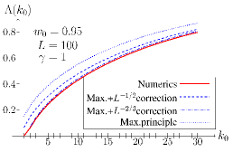
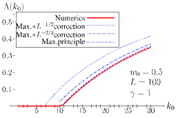
Figure 1: Growth rate $\Lambda$ as a function of the plateau width $k_{0}$ for two values of the plateau height $w_{0}=0.5,0.95$. The sequence length is $L=100$ and the mutation rate per sequence is $\gamma=1$. The solution of the maximum principle together with the $L^{-1/2}$-correction term (including the position-dependent mass) provides the best agreement with the numerics. The numerical values of the growth rate have been obtained by (numerical) calculation of the largest eigenvalue of the matrix defined by equation (2).

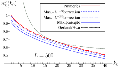
Figure 2: Critical plateau height as a function of the plateau width $k_{0}$. The sequence length is $L=500$ the mutation rate per sequence $\gamma=1$. The solution of the maximum principle together with the $L^{-1/2}$-correction term provides the best agreement with the numerics. With increasing $x_{0}$, the $L^{-2/3}$ and $L^{-1/2}$-corrections approach each other. The numerical values have been obtained by monitoring the average magnetization $M$ defined in (34) and determining the plateau height, where $M$ jumps from a finite value to zero. The slight modulation of the red line arises from the finite numerical resolution of this procedure.

3.6 Numerical results

To test the analytical predictions derived in the preceding subsections, we have carried out a detailed numerical study of the dependence of $\Lambda$ and $w_{0}^{c}$ on $k_{0}$, $L$ and $\gamma$. In figure 1 we show two examples for the dependence of $\Lambda$ on the plateau width $k_{0}$. The prediction of the asymptotic maximum principle (4) reproduces the qualitative behavior of the numerical data but significantly overestimates the value of $\Lambda$. The $L^{-2/3}$ finite size correction (23) derived in the harmonic approximation improves the comparison, but quantitative agreement is achieved only using the refined expression (31), which is proportional to $L^{-1/2}$.

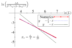
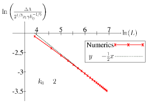
Figure 3: Illustration of the power of the sequence length in the correction term for fixed relative and absolute plateau width. $\Delta\Lambda$ is the numerical value for the growth rate $\Lambda_{num}$ less the value obtained from the maximum principle, eq. (4). For fixed relative plateau width, as well as for fixed absolute width, the numerics show the same exponent of the sequence length as the corresponding analytical result.

Figure 2 shows a similar comparison for the critical plateau height $w_{0}^{c}$. Here the prediction (26) of GH is also included and seen to match the numerical outcome only poorly, whereas the MP result with the finite size correction (31) produces excellent agreement. Finally, in left panel of figure 3 we verify that the finite size correction $\Delta\Lambda$ indeed varies as $L^{-2/3}$ when $L$ is increased at fixed relative plateau width $x_{0}$. The right panel shows the corresponding $L^{-1/2}$ dependence for fixed absolute plateau width $k_{0}$.

4 Fitness landscapes with competing peaks

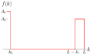
Figure 4: Illustration of a fitness landscape with two plateaus. This type of landscape is used to investigate the influence of height and (relative) broadness of the plateaus on the population fitness $\Lambda$.

4.1 The selection transition

Since we have validated the analytical results of section 3 via numerical studies, we can now apply the analytical theory to the phenomenon of the survival of the flattest as explained in the introduction. To be specific, we want to find out whether a broad plateau outcompetes a smaller but higher one even in the limit of long sequences.

In the literature this question has already been discussed to some extent by Schuster and Swetina [7]. The question can be answered by investigating a fitness landscape consisting of two fitness plateaus at the opposing ends of the Hamming space (see figure 4). As was shown in [7], for small $\mu$ the interference between the two plateaus is negligible when they are separated by a few mutational distances. The stationary state of the system is therefore to a very good approximation determined by the comparison between the population growth rates associated with each of the two plateaus in isolation.

Observing the center of mass of the population as function of the mutation rate and for fixed sequence length, we find two types of transitions. The first one is a jump of the population from the higher to the broader plateau, which we will refer to as the selection transition [23] taking place at a mutation rate $\mu_{s}$. The second transition is the well-known error threshold taking place at $\mu_{tr}$, where the population becomes uniformly spread in sequence space. To analyze these transitions, an order parameter is needed. A convenient quantity is the population averaged “magnetization” defined by

$$M=1-2\langle x\rangle\in[-1,1]\;\;\textrm{with}\;\;\langle x\rangle=\frac{1}{L}\sum_{k=0}^{L}kP^{\ast}_{k}.$$ (34)

If the whole population consists only of master sequences, the magnetization is $M=1$. If only the inverse master sequence is present, the magnetization becomes $M=-1$. For a uniform distribution in sequence space (delocalized population) the magnetization is $M=0$. Thus we can distinguish the qualitatively different states of the population in the two plateau landscape by considering the population averaged magnetization $M$ as a function of $\mu$.

As can be seen from figure 5, the selection transition (the jump between the two plateaus) is sharp even for finite sequence lengths, whereas the error threshold is a continuous transition for finite sequence length and only becomes sharp in the limit of infinite sequence length [23]. With growing sequence length the two critical mutation rates $\mu_{s}$ and $\mu_{tr}$ become smaller and also approach each other until, at a critical sequence length $L^{\ast}$, the selection transition completely disappears. For sequences longer than $L^{\ast}$, the population delocalizes directly from the high, narrow peak and the low, broad plateau is never substantially populated.

With the help of the maximum principle, this surprising behavior can be easily understood. Using (4), the selection threshold is obtained by equating the population mean fitness for the two competing peaks, which yields

$$\mu_{s}=\frac{w_{0}-w_{1}}{2\left(\sqrt{k_{1}L-k_{1}^{2}}-\sqrt{k_{0}L-k_{0}^{2}}\right)}\approx\frac{w_{0}-w_{1}}{2(\sqrt{k_{1}}-\sqrt{k_{0}})}L^{-1/2},$$ (35)

where $k_{0},k_{1}\ll L$ has been assumed in the last step. On the other hand, the error threshold $\mu_{tr}^{(i)}$ associated with plateau $i=0,1$ is determined by the vanishing of the corresponding principal eigenvalue $\Lambda_{i}$, which gives

$$\mu_{tr}^{(i)}=\frac{w_{i}}{L\left(1-2\sqrt{k_{i}L-k_{i}^{2}}\right)}\approx\frac{w_{i}}{1-2\sqrt{k_{i}/L}}L^{-1}.$$ (36)

The different scaling of the two types of thresholds with sequence length implies that for large $L$ the error threshold of the higher peak is encountered before the selection threshold, which therefore is no longer observable. The critical sequence length $L^{\ast}$ where the selection transition vanishes can be estimated by equating the approximate expressions (35) and (36), which yields

$$L^{\ast}\approx\frac{4(w_{0}\sqrt{k_{1}}-w_{1}\sqrt{k_{0}})^{2}}{(w_{0}-w_{1})^{2}}.$$ (37)

Following [7, 23], in our numerical work we have considered short plateaus, $k_{0}=1$ and $k_{1}=2$, with relative fitness values $w_{1}/w_{0}=0.9$, for which (37) give $L^{\ast}\approx 106$. Comparison with the numerical values for the selection and error thresholds in figure 6 shows that this significantly underestimates the value of $L^{\ast}$; moreover, the agreement between theory and numerics is not substantially improved by using the full expressions for the principal eigenvalues $\Lambda_{0}$ and $\Lambda_{1}$, including the $L^{-1/2}$-correction derived in subsection 3.5. This is not surprising, as the continuum approach developed in section 3 cannot be expected to be quantitatively accurate for plateaus sizes of order unity.

For completeness we mention that for plateau widths scaling with the sequence length (such that $x_{0}=k_{0}/L$ and $x_{1}=k_{1}/L$ are kept fixed as $L\to\infty$) the selection transition is maintained at a fixed value of $\gamma$ [18].

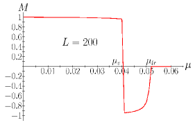
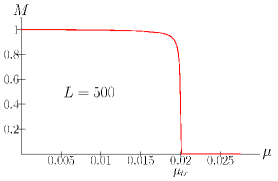
Figure 5: Order parameter $M$ as function of the mutation rate $\mu$ per site for a fitness landscape with a high plateau at $k=0$ and a broad plateau at $k=L$. For short sequence lengths one can observe a hopping of the population from the higher to the broader plateau and then a delocalization (left picture). For long sequences, one only observes the delocalization transition from the higher fitness plateau (right picture). The hopping between the plateaus we call the selection transition. It takes place at mutation rate $\mu_{s}$. The delocalization transition, also called error threshold, takes place at a mutation rate $\mu_{tr}$. The underlying fitness landscape is $w_{k}=10\cdot\Theta(1-k)+9\cdot\Theta(k-(L-2))$.

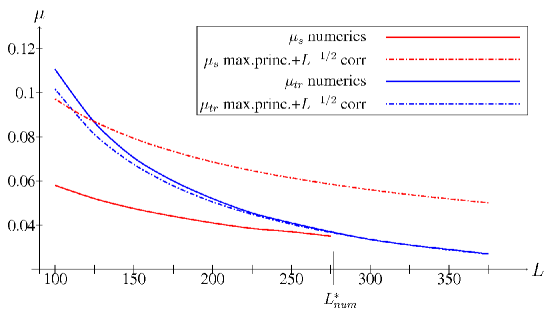
Figure 6: Critical mutation rate $\mu_{s}$ of the selection transition and $\mu_{tr}$ of the error threshold for the fitness landscape $w_{k}=10\cdot\Theta(1-k)+9\cdot\Theta(k-(L-2))$ as functions of the sequence length. The two lines cross at a critical sequence length $L^{\ast}$. The selection transition is observed only for sequence lengths smaller than $L^{\ast}$. The numerical data are compared to analytic predictions based on the MP including the $L^{-1/2}$-correction term. As before, the numerical values have been obtained by calculating the magnetization of the population and determining for each sequence length the mutation rate where the magnetization jumps.

4.2 The ancestral distribution

In addition to the equilibrium population distribution $P^{\ast}_{k}$ attained at long times, we can also consider the ancestral distribution, the equilibrium distribution of the backward time process, as introduced by Baake and collaborators [16, 21]. The ancestral distribution $a_{k}$ gives information on the origin of the equilibrium population and is obtained as the product of the right eigenvector $P^{\ast}_{k}$ and the left eigenvector $P^{\ast\ast}_{k}$ of the mutation-selection matrix defined through (2), $a_{k}\sim P^{\ast}_{k}\cdot P^{\ast\ast}_{k}$.

For the fitness landscape with two competing peaks, we find an ancestral population that is either located on one of the plateaus or uniformly distributed in sequence space (figure 7). The transitions beween these states are all of first order. The continuous character of the error threshold transition of the equilibrium population distribution, as opposed to the discontinuous transition of the ancestral distribution, can be explained by the growing mutational pressure affecting the population on the plateau and driving it towards the middle of the Hamming space. Mutations cause the population to ”leak out” from the plateau. Nevertheless, the individuals maintaining the population and compensating for the mutational loss are the ones with highest fitness, which are located on the plateau and make up the ancestral distribution.

Before closing the analysis of plateau-shaped fitness landscapes, we want to mention the connection between our description and the popular language of Ising chains or semi-infinite Ising models [27, 28]. In the Ising picture, the ancestral distribution becomes the bulk distribution on a semi-infinite two-dimensional (spatial or spatio-temporal) lattice, and the equilibrium distribution becomes the distribution in the surface layer. This analogy can be seen very clearly in the paper by Tarazona [23], where the different orders of the transitions in the two distributions are explained in terms of surface wetting.

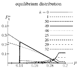
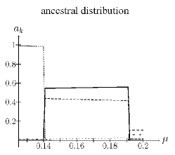
Figure 7: The dominant entries of the equilibrium and ancestral population distribution as a function of the mutation rate per site, calculated numerically. The underlying fitness landscape is the same two-plateau landscape used in figures 5 and 6. The sequence length is chosen as $L=50$. Occupation fractions are plotted only for the most populated Hamming classes. The two distributions undergo phase transitions at the same mutation rates, but at the error threshold the ancestral distribution undergoes a discontinuous transition, while for the equilibrium distribution the transition is continuous.

5 Epistasis and the error threshold

So far, we have discussed robustness of phenotypes using plateau-shaped fitness landscapes, which are a special case of the class of epistatic fitness functions. We now want to discuss the latter in a more general framework. Epistasis describes the non-linear dependence of the fitness function on the number of mismatches $k$ [13]. Every additional mismatch is penalized harder (synergistic epistasis of deleterious mutations) or less hard (diminishing epistasis) than the previous one. Here we address the effect of epistasis on the existence of an error threshold, which is defined for our purposes as a singularity in the dependence of the population mean fitness on the mutation rate. In general (but not always, see below) such a singularity is associated with a discontinuous jump in the location of the most populated genotype.

Following Wiehe [14] we consider the class of permutation invariant (Malthusian) epistatic fitness functions

$$w_{k}=w_{0}-bk^{\alpha},$$ (38)

where $k$ is again the Hamming distance to the master sequence and $b>0$. The epistasis exponent $\alpha$ takes the value $\alpha=1$ in the non-epistatic case, while $\alpha>1$ and $\alpha<1$ produces landscapes with synergistic and diminishing epistasis, respectively. For $\alpha\to 0$ (38) reduces to the sharp peak landscape $w_{k}=w_{0}-b(1-\delta_{k,0})$. It is well known that an error threshold exists for $\alpha\rightarrow 0$, but not for $\alpha=1$ [6]. Neglecting backward mutations, Wiehe argued in [14] that an error threshold emerges whenever $\alpha<1$. In the following we show that, based on the maximum principle (4), the critical value of the epistasis exponent below which an error threshold develops is in fact $\alpha=1/2$.

As before, we work in the scaling limit $L\to\infty$ and $\mu\to 0$ with the mutation rate per sequence $\gamma=\mu L=const$. In order to cast (38) into the form (3) required for the application of the maximum principle, we write

$$w_{k}=f(x)=w_{0}-\tilde{b}x^{\alpha},\;\;\;\;\mathrm{with}\;\;x=k/L,\;\;\;\;\tilde{b}=bL^{\alpha}$$ (39)

and the limit $L\rightarrow\infty$ should be combined with $b\rightarrow 0$, such that $\tilde{b}=const$. Since $b$ can be interpreted as a kind of selection coefficient, we are thus considering a situation where both the mutation rate (per site) and the selection forces are small. Applying the maximum principle (4) to this landscape, the mean fitness $\Lambda$ of the population in the equilibrium state is given by

$$\Lambda=\max_{x\in[0,1]}\{w_{0}-\tilde{b}x^{\alpha}-\gamma[1-2\sqrt{x(1-x)}]\}\equiv\max_{x\in[0,1]}\lambda(x),$$ (40)

where $\lambda(x)$ is the function inside the curly brackets.

To find the condition under which the maximum is attained inside the interval $x\in(0,1)$, we set $d\lambda/dx=0$, yielding the condition

$$\frac{\gamma}{\tilde{b}}(1-2x)=\alpha x^{\alpha-1/2}\sqrt{1-x}.$$ (41)

For $\alpha>1/2$ the right hand side is a convex function which vanishes at $x=0,1$, with an infinite slope at $x=1$. As a consequence, there exists always a unique solution $x_{c}\in(0,1)$ for any value of $\gamma/\tilde{b}$, which describes the location of the population for $L\to\infty$. The location varies smoothly from $x_{c}=0$ for $\gamma/\tilde{b}\to 0$ to $x_{c}\to 1/2$ for $\gamma/\tilde{b}\to\infty$, and there is no error threshold. However, for $\alpha<1/2$ the right hand side diverges at $x=0$, and there is no solution for small $\gamma/\tilde{b}$. The function $\lambda(x)$ is then monotonically decreasing, which implies that the maximum in (40) is located at the boundary point $x=0$ over a finite interval of $\gamma/\tilde{b}$. Increasing $\gamma/\tilde{b}$ the function $\lambda(x)$ develops a local maximum, which eventually exceeds the boundary value $\lambda(0)=w_{0}-\gamma$. At this point the population discontinuously delocalizes to an interior point $x_{c}\in(0,1)$. The error threshold condition is of the form $\gamma/\tilde{b}=g(\alpha)$ where the function $g(\alpha)$ is not explicitly available. This translates into the expression

$$\mu_{tr}=\frac{\gamma_{tr}}{L}=\frac{\tilde{b}g(\alpha)}{L}=g(\alpha)bL^{\alpha-1},$$ (42)

for the critical mutation rate $\mu_{tr}$. This scaling of $\mu_{\tr}$ with $L$ was also obtained in [14]. In the sharp peak limit $\alpha\to 0$ the threshold occurs at $\gamma/\tilde{b}=\gamma/b=1$, which implies that $g(0)=1$. On the other hand, for $\alpha=1/2$ the expansion of $\lambda(x)$ near $x=0$ reads

$$\lambda(x)\approx w_{0}-(\tilde{b}-2\gamma)x^{1/2}-\gamma x^{3/2},$$ (43)

which shows that $g(1/2)=1/2$. For $\gamma/\tilde{b}>1/2$ an interior maximum appears at $x_{c}=(2-\tilde{b}/\gamma)/3$, which moves continuously away from $x=0$. In the language of phase transitions, $\alpha=1/2$ can thus be viewed as a critical endpoint terminating the line of discontinuous phase transitions that occur for $\alpha<1/2$.

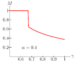
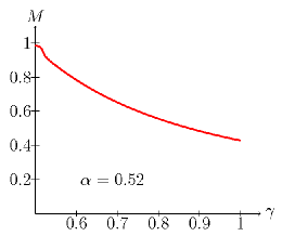
Figure 8: Magnetization as a function of mutation rate for the fitness landscape (38) with epistasis exponent $\alpha=0.4$ and $\alpha=0.52$, respectively. For $\alpha=0.4$ the magnetization undergoes a discontinuous jump, whereas for $\alpha=0.52$, it changes smoothly. Calculations have been done for a sequence length of $L=500$.

These predictions are fully confirmed by numerical calculations for finite sequence length. Figure 8 illustrates the existence of an error threshold for $\alpha<1/2$ and its absence for $\alpha>1/2$ by showing the behavior of the magnetization $M$ as a function of $\gamma$ for two different cases. The magnetization displays a non-analytic jump for $\alpha<1/2$ and varies smoothly for $\alpha>1/2$. In figure 9 we show the error threshold as a function $\gamma/\tilde{b}=g(\alpha)$, which interpolates between the limits $g(0)=1$ and $g(1/2)=1/2$.

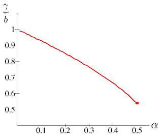
Figure 9: Numerically determined phase diagram for the epistatic fitness landscape (38). At the thick line the population undergoes a first order phase transition from a state localized at $x_{c}=0$ (below the line) to a delocalized state $x_{c}>0$ (above the line). This line terminates in a second order phase transition at $\alpha=1/2$. The deviation from the prediction $\gamma/\tilde{b}=g(1/2)=1/2$ at $\alpha=1/2$ is due to finite sequence length corrections. For all larger values of the epistasis exponent, $\alpha>1/2$, the population changes smoothly. Calculations have been performed for a sequence lengths of $L=750$. The slight modulation of the line is due to the finite numerical step size.

It should have become clear that the special role of $\alpha=1/2$ derives from the fact that for this value the leading order behavior of the fitness function for small $x$ matches that of the “entropic” term $\sim\sqrt{x(1-x)}$ in the maximum principle (4). Since a similar term appears also for general alphabet sizes [see (50)], the considerations of this section hold in that case as well.

6 Conclusions

In this paper we discussed the properties of epistatic fitness landscapes, with particular emphasis on mesa landscapes describing mutational robustness of phenotypes, which have been studied previously in the context of regulatory motifs [3, 4]. As population evolution model we used the continuous time Crow-Kimura model, which is a quasispecies model for asexual and haploid organisms, and analysed its stationary states for sequences consisting of two letters. As explained in Appendix B, it is straightforward to generalize our results to sequence alphabets of general size. Similarly, the extension to discrete time dynamics can be carried out by replacing the Malthusian fitness landscape $w_{k}$ by its Wrightian counterpart $W_{k}\sim\exp(w_{k})$ [6, 18, 19].

We reviewed two existing approaches [3, 16, 18] to this problem and explained the discrepancy between their predictions by extending the approach of Gerland and Hwa [3] beyond the harmonic approximation. Based on a quantum mechanical analogy we derived a novel finite size correction term to the maximum principle of [16], which significantly improves the agreement with numerical calculations. Our central result is that the relative number of tolerable mismatches $x_{0}=k_{0}/L$ is the relevant parameter for the fitness effect of mutational robustness, and we provide accurate formulae for its quantitative evaluation. As a consequence, we showed that the selection transition first described by Schuster and Swetina [7] disappears for long sequences.

Finally, in section 5, we discussed more general forms of epistatic fitness landscapes with regard to the existence of an error threshold. Based on the results of [16, 21] we improved on earlier work [14] and showed that diminishing epistasis [$\alpha<1$ in the fitness function (38)] is not a sufficient condition for an error threshold to occur.

Appendix A: The large deviations approach

We start by symmetrizing the eigenvalue problem (2). The discrete analogue of the transformation (14) is

$$Q_{k}={L\choose k}^{1/2}P^{\ast}_{k},$$ (44)

which leads to

$$\Lambda Q_{k}=(w_{k}-\gamma)Q_{k}+\mu\sqrt{(L-k)(k+1)}\,Q_{k+1}+\mu\sqrt{(L-k+1)k}\,Q_{k-1}.$$ (45)

Following [20], we now perform the continuum limit by making a large deviations ansatz for $Q_{k}$,

$$Q_{k}=Q_{xL}=\psi(x)=\exp[-\epsilon^{-1}u(x)]$$ (46)

with $\epsilon=1/L$. Inserting this into (45) one finds

$$(\Lambda-f(x)+\gamma)\psi=2\gamma\sqrt{x(1-x)}\cosh[u^{\prime}]\psi.$$ (47)

Cancelling $\psi$ on both sides yields a Hamilton-Jacobi equation for the ‘action’ $u(x)$, with $u^{\prime}=du/dx$ playing the role of a canonical momentum [20]. In order to cast (47) into the form of a Schrödinger equation, we expand the momentum-dependent factor to quadratic order, $\cosh(u^{\prime})\approx 1+(u^{\prime})^{2}/2$, and make use of the relation

$$(u^{\prime})^{2}=\epsilon^{2}\psi^{-1}\frac{d^{2}\psi}{dx^{2}},$$ (48)

which follows from (46) to leading order in $\epsilon$. Inserting this into (47) results in (28).

Appendix B: General alphabet size

Here we show how our results generalize to the case where the symbols in the genetic sequence are taken from an alphabet of $A>2$ letters (for nucleotide sequences $A=4$). We assume a uniform point mutation rate $\mu$ connecting any two of the $A$ possible states of a site in the sequence, and a fitness function $w_{k}$ that depends on the relative number of mismatches according to (3). It is then straightforward to see that the basic eigenvalue problem (2) generalizes to

$$(\Lambda-w_{k})P^{\ast}_{k}=$$ (49)

$$=(A-1)\gamma\left[\frac{k+1}{A-1}P^{\ast}_{k+1}+(L-k+1)P^{\ast}_{k-1}-\left(L-k+\frac{k}{A-1}\right)P^{\ast}_{k}\right].$$

Applying the results of [17, 29, 30] to this problem we find that, asymptotically for large $L$, the principal eigenvalue is given by the maximum principle

$$\Lambda=\max_{x\in[0,1]}\left\{f(x)-(A-1)\gamma\left[\left(1-\frac{(A-2)x}{A-1}\right)-\frac{2\sqrt{x(1-x)}}{\sqrt{A-1}}\right]\right\}.$$ (50)

For the case of the mesa landscape (6) this implies that the population is localized near the optimal genotype for $w_{0}>w_{0}^{c}$ with

$$w_{0}^{c}=\gamma(A-1)\left[1-\frac{(A-2)x_{0}}{A-1}-\frac{2\sqrt{x_{0}(1-x_{0})}}{\sqrt{A-1}}\right].$$ (51)

The right hand side is a monotonically decreasing function of $x_{0}$ which vanishes at $x_{0}=1-1/A$. For fixed $x_{0}$ it is an increasing function of $A$.

References

References

- [1] J. A. G. M. de Visser et al. Perspective: Evolution and detection of genetic robustness. Evolution, 57:1959–1972, 2003.
- [2] D. C. Krakauer and J. B. Plotkin. Redundancy, antiredundancy, and the robustness of genomes. Proc. Nat. Acad. Sci. USA, 99:1405–1409, 2002.
- [3] U. Gerland and T. Hwa. On the selection and evolution of regulatory DNA motifs. J. Mol. Evol., 55:386–400, 2002.
- [4] J. Berg, S. Willmann, and M. Lässig. Adaptive evolution of transcription factor binding sites. BMC Evolutionary Biology, 4:42, 2004.
- [5] L. Peliti. Quasispecies evolution in general mean-field landscapes. Europhysics Letters, 57:745, 2002.
- [6] K. Jain and J. Krug. Adaptation in simple and complex fitness landscapes. In U. Bastolla, M. Porto, H. E. Roman, and M. Vendruscolo, editors, Structural approaches to sequence evolution: Molecules,networks and populations. Springer, Berlin, 2007.
- [7] P. Schuster and J. Swetina. Stationary mutant distributions and evolutionary optimization. Bulletin of Mathematical Biology, 50:635–660, 1988.
- [8] C. O. Wilke, J. L. Wang, C. Ofria, R. E. Lenski, and C. Adami. Evolution of digital organisms at high mutation rates leads to survival of the flattest. Nature, 412:331–333, 2001.
- [9] F. M. Codoner, J.-A. Daros, R. V. Solé, and S. F. Elena. The fittest versus the flattest: Experimental confirmation of the quasispecies effect with subviral pathogens. PLoS Pathogens, 2:e136, 2006.
- [10] R. Sanjuan, J. M. Cuevas, V. Furio, E. C. Holmes, and A. Moya. Selection for robustness in mutagenized RNA viruses. PLoS Genetics, 3:e93, 2007.
- [11] M. Rolland, C. Brander, D. C. Nickle, J. T. Herbeck, G. S. Gottlieb, M. S. Campbell, B. S. Maust, and J. I. Mullins. HIV-1 over time: fitness loss or robustness gain? Nature Reviews Microbiology, 5, 2007.
- [12] J. Sardanyés, S.F. Elena, and R.V. Solé. Simple quasispecies models for the survival-of-the-flattest effect: The role of space. J. Theor. Biol., 250:560–568, 2008.
- [13] P. C. Phillips, S. P. Otto, and M. C. Whitlock. Beyond the average: The evolutionary importance of gene interactions and variability of epistatic effects. In J. B. Wolf, E. D. Brodie III, and M. J. Wade, editors, Epistasis and the evolutionary process. Oxford University Press, Oxford, 2000.
- [14] T. Wiehe. Model dependency of error thresholds: the role of fitness functions and contrasts between the finite and infinte sites models. Genet. Res. Camb., 69:127–136, 1997.
- [15] K. Jain. Loss of least-loaded class in asexual populations due to drift and epistasis. Genetics, 179:2125, 2008.
- [16] J. Hermisson, O. Redner, H. Wagner, and E. Baake. Mutation-selection balance: Ancestry, load, and maximum principle. Theor. Pop. Biol., 62:9–46, 2002.
- [17] E. Baake, M. Baake, A. Bovier, and M. Klein. An asymptotic maximum principle for essentially linear evolution models. J. Math. Biol., 50:83–114, 2005.
- [18] D. B. Saakian and C.-K. Hu. Exact solution of the Eigen model with general fitness functions and degradation rates. Proc. Nat. Acad. Sci. USA, 103:4935–4939, 2006.
- [19] J. M. Park and M. W. Deem. Schwinger boson formulation and solution of the Crow-Kimura and Eigen models of quasispecies theory. J. Stat. Phys., 125:975, 2006.
- [20] D. B. Saakian. A new method for the solution of model of biological evolution: Derivation of exact steady-state distributions. J. Stat. Phys., 128:781–798, 2007.
- [21] E. Baake and H.-O. Georgii. Mutation, selection, and ancestry in branching models: a variational approach. J. Math. Biol., 54:257, 2007.
- [22] K. Sato and K. Kaneko. Evolution equation of phenotype distribution: General formulation and application to error catastrophe. Phys. Rev. E, 75:061909, 2007.
- [23] P. Tarazona. Error thresholds for molecular quasispecies as phase transitions: From simple landscapes to spin-glass models. Phys. Rev. A, 45:6038, 1992.
- [24] C. J. Thompson and J. L. McBride. On Eigen’s theory of the self-organization of matter and the evolution of biological macromolecules. Mathematical Biosciences, 21:127, 1974.
- [25] D. Sornette. Critical Phenomena in Natural Sciences. Springer, Berlin, 2000.
- [26] H. Rollnik. Quantentheorie I. Vieweg, Wiesbaden, 1995.
- [27] I. Leuthäusser. Statistical mechanics of Eigen’s evolution model. J. Stat. Phys., 48:343, 1987.
- [28] E. Baake and H. Wagner. Mutation-selection models solved exactly with methods from statistical mechanics. Genet. Res., 78:93, 2001.
- [29] T. Garske and U. Grimm. A maximum principle for the mutation-selection equilibrium of nucleotide sequences. Bull. Math. Biol., 66:397, 2004.
- [30] T. Garske and U. Grimm. Maximum principle and mutation thresholds for four-letter sequence evolution. J. Stat. Mech., P07007, 2004.